On EM algorithms and their proximal generalizations

Abstract

In this paper, we analyze the celebrated EM algorithm from the point of view of proximal point algorithms. More precisely, we study a new type of generalization of the EM procedure introduced in [4] and called Kullback-proximal algorithms. The proximal framework allows us to prove new results concerning the cluster points. An essential contribution is a detailed analysis of the case where some cluster points lie on the boundary of the parameter space.

1 Introduction

The problem of maximum likelihood (ML) estimation consists of finding a solution of the form

$$\theta_{ML}={\rm argmax}_{\theta\in\Theta}\;l_{y}(\theta),$$ (1)

where $y$ is an observed sample of a random variable $Y$ defined on a sample space $\mathcal{Y}$ and $l_{y}(\theta)$ is the log-likelihood function defined by

$$l_{y}(\theta)=\log g(y;\theta),$$ (2)

defined on the parameter space $\Theta\subset\mathbb{R}^{n}$, and $g(y;\theta)$ denotes the density of $Y$ at $y$ parametrized by the vector parameter $\theta$.

The Expectation Maximization (EM) algorithm is an iterative procedure which is widely used for solving ML estimation problems. The EM algorithm was first proposed by Dempster, Laird and Rubin [8] and has seen the number of its potential applications increase substantially since its appearance. The book of McLachlan and Krishnan [14] gives a comprehensive overview of the theoretical properties of the method and its applicability.

The convergence of the sequence of EM iterates towards a maximizer of the likelihood function was claimed in the original paper [8] but it was later noticed that the proof contained a flaw. A careful convergence analysis was finally given by Wu [21] based on Zangwill’s general theory [23]; see also [14]. Zangwill’s theory applies to general iterative schemes and the main task when using it is to verify that the assumptions of Zangwill’s theorems are satisfied. Since the appearance of Wu’s paper, convergence of the EM algorithm is often taken for granted in many cases where the necessary assumptions were sometimes not carefully justified. As an example, an often neglected issue is the behavior of EM iterates when they approach the boundary of the domain of definition of the functions involved. A different example is the following. It is natural to try and establish that EM iterates actually converge to a single point $\theta^{*}$, which involves proving uniqueness of the cluster point. Wu’s approach, reported in [14, Theorem 3.4, p. 89] is based on the assumption that the euclidean distance between two successive iterates tends to zero. However such an assumption is in fact very hard to verify in most cases and should not be deduced solely from experimental observations.

The goal of the present paper is to propose an analysis of EM iterates and their generalizations in the framework of Kullback proximal point algorithms. We focus on the geometric conditions that are provable in practice and the concrete difficulties concerning convergence towards boundaries and cluster point uniqueness. The approach adopted here was first proposed in [4] in which it was shown that the EM algorithm could be recast as a Proximal Point algorithm. A proximal scheme for maximizing the function $l_{y}(\theta)$ using the distance-like function $I_{y}$ is an iterative procedure of the form

$$\theta^{k+1}\in{\rm argmax}_{\theta\in\Omega}l_{y}(\theta)-\beta_{k}I_{y}(\theta,\theta^{k}),$$ (3)

where $(\beta_{k})_{k\in\mathbb{N}}$ is a sequence of positive real numbers often called relaxation parameters. Proximal point methods were introduced by Martinet [13] and Rockafellar [17] in the context of convex minimization. The proximal point representation of the EM algorithm [4] is obtained by setting $\beta_{k}=1$ and $I_{y}(\theta,\theta^{k})$ to the Kullback distance between some well specified conditional densities of a complete data vector. The general case of $\beta_{k}>0$ was called the Kullback Proximal Point algorithm (KPP). This approach was further developed in [5] where convergence was studied in the twice differentiable case with the assumption that the limit point lies in the interior of the domain. The main novelty of [5] was to prove that relaxation of the Kullback-type penalty could ensure superlinear convergence which was confirmed by experiment for a Poisson linear inverse problem. This paper is an extension of these previous works that addresses the problem of convergence under general conditions.

The main results of this paper are the following. Firstly, we prove that all the cluster points of the Kullback proximal sequence which lie in the interior of the domain are stationary points of the likelihood function $l_{y}$ under very mild assumptions that are easily verified in practice. Secondly, taking into account finer properties of $I_{y}$, we prove that every cluster point on the boundary of the domain satisfies the Karush-Kuhn-Tucker necessary conditions for optimality under nonnegativity constraints. To illustrate our results, we apply the Kullback-proximal algorithm to an estimation problem in animal carcinogenicity introduced in [1] in which an interesting nonconvex constraint is handled. In this case, the M-step cannot be obtained in closed form. However, the Kullback-proximal algorithm can be analyzed and implemented. Numerical experiments are provided which demonstrate the ability of the method to significantly accelerate the convergence of standard EM.

The paper is organized as follows. In Section 2, we review the Kullback proximal point interpretation of EM. Then, in Section 3 we study the properties of interior cluster points. We prove that such cluster points are in fact global maximizers of a certain penalized likelihood function. This allows us to justify using a relaxation parameter $\beta$ when $\beta$ is sufficiently small to permit avoiding saddle points. Section 4 pursues the analysis in the case where the cluster point lies on a boundary of the domain of $I_{y}$.

2 The Kullback proximal framework

In this section, we review the EM algorithm and the Kullback proximal interpretation discussed in [5].

2.1 The EM algorithm

The EM procedure is an iterative method which produces a sequence $(\theta^{k})_{k\in\mathbb{N}}$ such that each $\theta^{k+1}$ maximizes a local approximation of the likelihood function in the neighborhood of $\theta^{k}$. This point of view will become clear in the proximal point framework of the next subsection.

In the traditional approach, one assumes that some data are hidden from the observer. A frequent example of hidden data is the class to which each sample belongs in the case of mixtures estimation. Another example is when the observed data are projection of an unkown object as for image reconstruction problems in tomography. One would prefer to consider the likelihood of the complete data instead of the ordinary likelihood. Since some parts of the data are hidden, the so called complete likelihood cannot be computed and therefore must be approximated. For this purpose, we will need some appropriate notations and assumptions which we now describe. The observed data are assumed to be i.i.d. samples from a unique random vector $Y$ taking values on a data space $\mathcal{Y}$. Imagine that we have at our disposal more informative data than just samples from $Y$. Suppose that the more informative data are samples from a random variable $X$ taking values on a space $\mathcal{X}$ with density $f(x;\theta)$ also parametrized by $\theta$. We will say that the data $X$ is more informative than the actual data $Y$ in the sense that $Y$ is a compression of $X$, i.e. there exists a non-invertible transformation $h$ such that $Y=h(X)$. If one had access to the data $X$ it would therefore be advantageous to replace the ML estimation problem (1) by

$$\hat{\theta}_{ML}={\rm argmax}_{\theta\in{\mathbb{R}}^{p}}l_{x}(\theta),$$ (4)

with $l_{x}(\theta)=\log f(x;\theta)$. Since $y=h(x)$ the density $g$ of $Y$ is related to the density $f$ of $X$ through

$$g(y;\theta)=\int_{h^{-1}(\{y\})}f(x;\theta)d\mu(x)$$ (5)

for an appropriate measure $\mu$ on $\mathcal{X}$. In this setting, the data $y$ are called incomplete data whereas the data $x$ are called complete data.

Of course the complete data $x$ corresponding to a given observed sample $y$ are unknown. Therefore, the complete data likelihood function $l_{x}(\theta)$ can only be estimated. Given the observed data $y$ and a previous estimate of $\theta$ denoted $\bar{\theta}$, the following minimum mean square error estimator (MMSE) of the quantity $l_{x}(\theta)$ is natural

$$Q(\theta,\bar{\theta})={\sf E}[\log f(x;\theta)|y;\bar{\theta}],$$

where, for any integrable function $F(x)$ on $\mathcal{X}$, we have defined the conditional expectation

$${\sf E}[F(x)|y;\bar{\theta}]=\int_{h^{-1}(\{y\})}F(x)k(x|y;\bar{\theta})d\mu(x)$$

and $k(x|y;\bar{\theta})$ is the conditional density function given $y$

$$k(x|y;\bar{\theta})=\frac{f(x;\bar{\theta})}{g(y;\bar{\theta})}.$$ (6)

Having described the notions of complete data and complete likelihood and its local estimation we now turn to the EM algorithm. The idea is relatively simple: a legitimate way to proceed is to require that iterate $\theta^{k+1}$ be a maximizer of the local estimator of the complete likelihood conditionally on $y$ and $\theta^{k}$. Hence, the EM algorithm generates a sequence of approximations to the solution (4) starting from an initial guess $\theta^{0}$ of $\theta_{ML}$ and is defined by

$$\text{\bf Compute }Q(\theta,\theta^{k})={\sf E}[\log f(x;\theta)|y;\theta^{k}]\text{\hskip 28.45274pt\bf E Step}$$

$$\theta^{k+1}={\rm argmax}_{\theta\in{\mathbb{R}}^{p}}Q(\theta,\theta^{k})\text{\hskip 82.51282pt\bf M Step}$$

2.2 Kullback proximal interpretation of the EM algorithm

Consider the general problem of maximizing a concave function $\Phi(\theta)$. The original proximal point algorithm introduced by Martinet [13] is an iterative procedure which can be written

$$\theta^{k+1}={\rm argmax}_{\theta\in D_{\Phi}}\left\{\Phi(\theta)-\frac{\beta_{k}}{2}\|\theta-\theta^{k}\|^{2}\right\}.$$ (7)

The quadratic penalty $\frac{1}{2}\|\theta-\theta^{k}\|^{2}$ is relaxed using a sequence of positive parameters $\{\beta_{k}\}$. In [17], Rockafellar showed that superlinear convergence of this method is obtained when the sequence $\{\beta_{k}\}$ converges towards zero.

It was proved in [5] that the EM algorithm is a particular example in the class of proximal point algorithms using Kullback Leibler types of penalties. One proceeds as follows. Assume that the family of conditional densities $\{k(x|y;\theta)\}_{\theta\in{\mathbb{R}}^{p}}$ is regular in the sense of Ibragimov and Khasminskii [9], in particular $k(x|y;\theta)\mu(x)$ and $k(x|y;\bar{\theta)}\mu(x)$ are mutually absolutely continuous for any $\theta$ and $\bar{\theta}$ in ${\mathbb{R}}^{p}$. Then the Radon-Nikodym derivative $\frac{k(x|y,\bar{\theta})}{k(x|y;\theta)}$ exists for all $\theta,\bar{\theta}$ and we can define the following Kullback Leibler divergence:

$$I_{y}(\theta,\bar{\theta})={\sf E}\bigl{[}\log\frac{k(x|y,\bar{\theta})}{k(x|y;\theta)}|y;\bar{\theta}\;\bigr{]}.$$ (8)

We are now able to define the Kullback-proximal algorithm. For this purpose, let us define $D_{l}$ as the domain of $l_{y}$, $D_{I,\theta}$ the domain of $I_{y}(\cdot,\theta)$ and $D_{I}$ the domain of $I_{y}(\cdot,\cdot)$.

Definition 2.2.1.

Let $(\beta_{k})_{k\in\mathbb{N}}$ be a sequence of positive real numbers. Then, the Kullback-proximal algorithm is defined by

$$\theta^{k+1}={\rm argmax}_{\theta\in D_{l}\cap D_{I,\theta^{k}}}l_{y}(\theta)-\beta_{k}I_{y}(\theta,\theta^{k}).$$ (9)

The main result on which the present paper relies is that EM algorithm is a special case of (9), i.e. it is a penalized ML estimator with proximal penalty $I_{y}(\theta,\theta^{k})$.

Proposition 2.2.2.

[5, Proposition 1] The EM algorithm is a special instance of the Kullback-proximal algorithm with $\beta_{k}=1$, for all $k\in\mathbb{N}$.

The previous definition of the Kullback proximal algorithm may appear overly general to the reader familiar with the usual practical interpretation of the EM algorithm. However, we found that such a framework has at least the three following benefits [5]:

• to our opinion, the convergence proof of our EM is more natural,

• the Kullback proximal framework may easily incorporate additional constraints, a feature that may be of crucial importance as demonstrated in the example of Section 5.1 below,

• the relaxation sequence $(\beta_{k})_{k\in\mathbb{N}}$ allows one to weight the penalization term and its convergence to zero implies quadratic convergence in certain examples.

The first of these three arguments is also supported by our simplified treatment of the componentwise EM procedure proposed in [3] and the remarkable recent results of [20] based on a special proximal entropic representation of EM for getting precise estimates on the convergence speed of EM algorithms, however, with much more restrictive assumptions than the ones of the present paper.

Although our results are obtained under mild assumptions concerning the relaxation sequence $(\beta_{k})_{k\in\mathbb{N}}$ including the case $\beta_{k}=0$, several precautions should be taken when implementing the method. However, one of the key features of EM-like procedures is to allow easy handling of positivity or more complex constraints, such as the ones discussed in the example of Section 5.1. In such cases the function $I_{y}$ behaves like a barrier whose value increases to infinity as the iterates approach the boundary of the constraint set. Hence, the sequence $(\beta_{k})_{k\in\mathbb{N}}$ ought to be positive in order to exploit this important computational feature. On the other hand, as proved under twice differentiability assumptions in [5] when the cluster set reduces to a unique nondegenerate maximizer in the interior of the domain of the log-likelihood and $\beta_{k}$ converges to zero, quadratic convergence is obtained. This nice behavior is not satisfied in the plain EM case where $\beta_{k}=1$ for all $k\in\mathbb{N}$. As a drawback, one problem in decreasing the $\beta_{k}$’s too quickly is possible numerical ill conditioning. The problem of choosing the relaxation sequence is still largely open. We have found however that for most ”reasonable” sequences, our method was at least as fast as the standard EM.

Finally, we would like to end our presentation of KPP-EM by noting that closed form iterations may not be available in the case $\beta_{k}\neq 1$. If this is the case, solving (9) becomes a subproblem which will require iterative algorithms. In some interesting examples, e.g. the case presented in Section 5.1. In this case, the standard EM iterations are not available in closed form in the first place and KPP-EM provides faster convergence while preserving monotonicity and constraint satisfaction.

2.3 Notations and assumptions

The notation $\|\cdot\|$ will be used to denote the norm on any previously defined space without more precision. The space on which it is the norm should be obvious from the context. For any bivariate function $\Phi$, $\nabla_{1}\Phi$ will denote the gradient with respect to the first variable. In the remainder of this paper we will make the following assumptions.

Assumptions 2.3.1.

(i) $l_{y}$ is differentiable on $D_{l}$ and $l_{y}(\theta)$ tends to $-\infty$ whenever $\|\theta\|$ tends to $+\infty$.
(ii) the projection of $D_{I}$ onto the first coordinate is a subset of $D_{l}$.
(iii) $(\beta_{k})_{k\in\mathbb{N}}$ is a convergent nonnegative sequence of real numbers whose limit is denoted by $\beta^{*}$.

We will also impose the following assumptions on the distance-like function $I_{y}$.

Assumptions 2.3.2.

(i) There exists a finite dimensional euclidean space $S$, a differentiable mapping $t:D_{l}\mapsto S$ and a functional $\Psi:D_{\Psi}\subset S\times S\mapsto\mathbb{R}$ such that

$$I_{y}(\theta,\bar{\theta})=\Psi(t(\theta),t(\bar{\theta})),$$

where $D_{\psi}$ denotes the domain of $\Psi$.
(ii) For any $\{t^{k},t)_{k\in\mathbb{N}}\}\subset D_{\Psi}$ there exists $\rho_{t}>0$ such that $\lim_{\|t^{k}-t\|\rightarrow\infty}I_{y}(t^{k},t)\geq\rho_{t}$. Moreover, we assume that $\inf_{t\in M}\rho_{t}>0$ for any bounded set $M\subset S$.
For all $(t^{\prime},t)$ in $D_{\Psi}$, we will also require that
(iii) (Positivity) $\Psi(t^{\prime},t)\geq 0$,
(iv) (Identifiability) $\Psi(t^{\prime},t)=0\Leftrightarrow t=t^{\prime}$,
(v) (Continuity) $\Psi$ is continuous at $(t^{\prime},t)$
and for all $t$ belonging to the projection of $D_{\Psi}$ onto its second coordinate,
(vi) (Differentiability) the function $\Psi(\cdot,t)$ is differentiable at $t$.

Assumptions 2.3.1(i) and (ii) on $l_{y}$ are standard and are easily checked in practical examples, e.g. they are satisfied for the Poisson and additive mixture models. Notice that the domain $D_{I}$ is now implicitly defined by the knowledge of $D_{l}$ and $D_{\Psi}$. Moreover $I_{y}$ is continuous on $D_{I}$. The importance of requiring that $I_{y}$ has the prescribed shape comes from the fact that $I_{y}$ might not satisfy assumption 2.3.2(iv) in general. Therefore assumption 2.3.2 (iv) reflects the requirement that $I_{y}$ should at least satisfy the identifiability property up to a possibly injective transformation. In both examples discussed above, this property is an easy consequence of the well known fact that $a\log(a/b)=0$ implies $a=b$ for positive real numbers $a$ and $b$. The growth, continuity and differentiability properties 2.3.2 (ii), (v) and (vi) are, in any case, nonrestrictive.

For the sake of notational convenience, the regularized objective function with relaxation parameter $\beta$ will be denoted

$$F_{\beta}(\theta,\bar{\theta})=l_{y}(\theta)-\beta I_{y}(\theta,\bar{\theta}).$$ (10)

Finally we make the following general assumption.

Assumptions 2.3.3.

The Kullback proximal iteration (9) is well defined, i.e. there exists at least one maximizer of $F_{\beta^{k}}(\theta,\theta^{k})$ at each iteration $k$.

In the EM case, i.e. $\beta=1$, this last assumption is equivalent to the computability of M-steps. A sufficient condition for this assumption to hold would be, for instance, that $F_{\beta}(\theta,\bar{\theta})$ be sup-compact, i.e. the level sets $\{\theta\mid F_{\beta}(\theta,\bar{\theta})\geq\alpha\}$ be compact for all $\alpha$, $\beta>0$ and $\bar{\theta}\in D_{l}$. However, this assumption is not usually satisfied since the distance-like function is not defined on the boundary of its domain. In practice it suffices to solve the equation $\nabla F_{\beta^{k}}(\theta,\theta^{k})=0$, to prove that the solution is unique. Then assumption 2.3.1(i) is sufficient to conclude that we actually have a maximizer.

2.4 General properties : monotonicity and boundedness

Using Assumptions 2.3.1, we easily deduce monotonicity of the likelihood values and boundedness of the proximal sequence. The first two lemmas are proved, for instance, in [5].

We start with the following monotonicity result.

Lemma 2.4.1.

[5, Proposition 2] For any iteration $k\in\mathbb{N}$, the sequence $(\theta^{k})_{k\in\mathbb{N}}$ satisfies

$$l_{y}(\theta^{k+1})-l_{y}(\theta^{k})\geq\beta_{k}I_{y}(\theta^{k},\theta^{k+1})\geq 0.$$ (11)

From the previous lemma, we easily obtain the boundedness of the sequence.

Lemma 2.4.2.

[5, Lemma 2] The sequence $(\theta^{k})_{k\in\mathbb{N}}$ is bounded.

The next lemma will also be useful.

Lemma 2.4.3.

Assume that there exists a subsequence $(\theta^{\sigma(k)})_{k\in\mathbb{N}}$ belonging to a compact set $C$ included in $D_{l}$. Then,

$$\lim_{k\rightarrow\infty}\beta_{k}I_{y}(\theta^{k+1},\theta^{k})=0.$$

Proof. Since $l_{y}$ is continuous over $C$, $\sup_{\theta\in C}l_{y}(\theta)<+\infty$ and $(l_{y}(\theta^{\sigma(k)}))_{k\in\mathbb{N}}$ is therefore bounded from above. Moreover, Lemma 2.4.1 implies that the sequence $(l_{y}(\theta^{k}))_{k\in\mathbb{N}}$ is monotone nondecreasing. Therefore, the whole sequence $(l_{y}(\theta^{k}))_{k\in\mathbb{N}}$ is bounded from above and convergent. This implies that $\lim_{k\rightarrow\infty}l_{y}(\theta^{k+1})-l_{y}(\theta^{k})=0$. Applying Lemma 2.4.1 again, we obtain the desired result. $\Box$

3 Analysis of interior cluster points

The convergence analysis of Kullback proximal algorithms is split into two parts, the first part being the subject of this section. We prove that if the accumulation points $\theta^{*}$ of the Kullback proximal sequence satisfy $(\theta^{*},\theta^{*})\in D_{I_{y}}$ they are stationary points of the log-likelihood function $l_{y}$. It is also straightforward to show that the same analysis applies to the case of penalized likelihood estimation.

3.1 Nondegeneracy of the Kullback penalization

We start with the following useful lemma.

Lemma 3.1.1.

Let $(\alpha_{1}^{k})_{k\in\mathbb{N}}$ and $(\alpha_{2}^{k})_{k\in\mathbb{N}}$ be two bounded sequences in $D_{\Psi}$ satisfying

$$\lim_{k\rightarrow\infty}\Psi(\alpha_{1}^{k},\alpha_{2}^{k})=0.$$

Assume that every couple $(\alpha_{1}^{*},\alpha_{2}^{*})$ of accumulation points of these two sequences lies in $D_{\Psi}$. Then,

$$\lim_{k\rightarrow\infty}\|\alpha_{1}^{k}-\alpha_{2}^{k}\|=0.$$

Proof. First, one easily obtains that $(\alpha_{2}^{k})_{k\in\mathbb{N}}$ is bounded (use a contradiction argument and Assumption 2.3.2 (ii)). Assume that there exits a subsequence $(\alpha_{1}^{\sigma(k)})_{k\in\mathbb{N}}$ such that $\|\alpha_{1}^{\sigma(k)}-\alpha_{2}^{\sigma(k)}\|\geq 3\epsilon$ for some $\epsilon>0$ and for all large $k$. Since $(\alpha_{1}^{\sigma(k)})_{k\in\mathbb{N}}$ is bounded, one can extract a convergent subsequence. Thus we may assume without any loss of generality that $(\alpha_{1}^{\sigma(k)})_{k\in\mathbb{N}}$ is convergent with limit $\alpha^{*}$. Using the triangle inequality, we have $\|\alpha_{1}^{\sigma(k)}-\alpha_{1}^{*}\|+\|\alpha_{1}^{*}-\alpha_{2}^{\sigma(k)}\|\geq 3\epsilon$. Since $(\alpha_{1}^{\sigma(k)})_{k\in\mathbb{N}}$ converges to $\alpha_{1}^{*}$, there exists a integer $K$ such that $k\geq K$ implies $\|\alpha_{1}^{\sigma(k)}-\alpha_{1}^{*}\|\leq\epsilon$. Thus for $k\geq K$ we have $\|\alpha_{1}^{*}-\alpha_{2}^{\sigma(k)}\|\geq 2\epsilon$. Now recall that $(\alpha_{2}^{k})_{k\in\mathbb{N}}$ is bounded and extract a convergent subsequence $(\alpha_{2}^{\sigma(\gamma(k))})_{k\geq K}$ with limit denoted by $\alpha_{2}^{*}$. Then, using the same arguments as above, we obtain $\|\alpha_{1}^{*}-\alpha_{2}^{*}\|\geq\epsilon$. Finally, recall that $\lim_{k\rightarrow\infty}\Psi(\alpha_{1}^{k},\alpha_{2}^{k})=0$. We thus have $\lim_{k\rightarrow\infty}\Psi(\alpha_{1}^{\sigma(\gamma(k))},\alpha_{2}^{\sigma(\gamma(k))})=0$, and, due to the fact that the sequences are bounded and $\Psi(\cdot,\cdot)$ is continuous in both variables, we have $I_{y}(\alpha_{1}^{*},\alpha_{2}^{*})=0$. Thus assumption 2.3.2 (iv) implies that $\|\alpha_{1}^{*}-\alpha_{2}^{*}\|=0$ and we obtain a contradiction. Hence, $\lim_{k\rightarrow\infty}\|\alpha_{1}^{k}-\alpha_{2}^{k}\|=0$ as claimed. $\Box$

3.2 Cluster points

The main results of this section are the following. First, we prove that under the assumptions 2.3.1, 2.3.2 and 2.3.3, any cluster point $\theta^{*}$ is a global maximizer of $F_{\beta^{*}}(\theta^{*},\theta^{*})$. We then use this general result to prove that such cluster points are stationary points of the log-likelihood function. This result motivates a natural assumption under which $\theta^{*}$ is in fact a local maximizer of $l_{y}$. In addition we show that if the sequence $(\beta^{k})_{k\in\mathbb{N}}$ converges to zero, i.e. $\beta^{*}=0$, then $\theta^{*}$ is a global maximizer of log-likelihood. Finally, we discuss some simple conditions under which the algorithm converges, i.e. has only one cluster point.

The following theorem states a result which describes the stationary points of the proximal point algorithm as global maximizers of the asymptotic penalized function.

Theorem 3.2.1.

Assume that $\beta^{*}>0$. Let $\theta^{*}$ be any accumulation point of $(\theta^{k})_{k\in\mathbb{N}}$. Assume that $(\theta^{*},\theta^{*})\in D_{I}$. Then, $\theta^{*}$ is a global maximizer of the penalized function $F_{\beta^{*}}(\cdot,\theta^{*})$ over the projection of $D_{I}$ onto its first coordinate, i.e.

$$F_{\beta^{*}}(\theta^{*},\theta^{*})\geq F(\theta,\theta^{*})$$

for all $\theta$ such that $(\theta,\theta^{*})\in D_{I}$.

An informal argument is as follows. Assume that $\Theta=\mathbb{R}^{n}$. From the definition of the proximal iterations, we have

$$F_{\beta_{\sigma(k)}}(\theta^{\sigma(k)+1},\theta^{\sigma(k)})\geq F_{\beta_{\sigma(k)}}(\theta,\theta^{\sigma(k)})$$

for all subsequence $(\theta^{\sigma(k)})_{k\in\mathbb{N}}$ converging to $\theta^{*}$ and for all $\theta\in\Theta$. Now, assume we can prove that $\theta^{\sigma(k)}$ also converges to $\theta^{*}$, we obtain by taking the limit and using continuity, that

$$F_{\beta_{*}}(\theta^{*},\theta^{*})\geq F_{\beta_{*}}(\theta,\theta^{*})$$

which is the required result. There are two major difficulties when one tries to transform this sketch into a rigorous argument. The first one is related to the fact that $l_{y}$ and $I_{y}$ are only defined on domains which may not to be closed. Secondly, proving that $\theta^{\sigma(k)}$ converges to $\theta^{*}$ is not an easy task. This issue will be discussed in more detail in the next section. The following proof overcomes both difficulties.

Proof. Without loss of generality, we may reduce the analysis to the case where $\beta_{k}\geq\beta>0$ for a certain $\beta$. The fact that $\theta^{*}$ is a cluster point implies that there is a subsequence of $(\theta^{k})_{k\in\mathbb{N}}$ converging to $\theta^{*}$. For $k$ sufficiently large, we may assume that the terms $(\theta^{\sigma(k+1)},\theta^{\sigma(k)})$ belong to a compact neighborhood $C^{*}$ of $(\theta^{*},\theta^{*})$ included in $D_{I}$. Recall that

$$F_{\beta_{\sigma(k)-1}}(\theta^{\sigma(k)},\theta^{\sigma(k)-1})\geq F_{\beta_{\sigma(k)-1}}(\theta,\theta_{\sigma(k)-1})$$

for all $\theta$ such that $(\theta,\theta^{\sigma(k)-1})\in D_{I}$ and a fortiori for $(\theta,\theta^{\sigma(k)-1})\in C^{*}$. Therefore,

$$\begin{array}[]{rl}F_{\beta^{*}}(\theta^{\sigma(k)},\theta^{\sigma(k)-1})&-(\beta_{k}-\beta^{*})I_{y}(\theta^{\sigma(k)},\theta^{\sigma(k)-1})\geq\\ &F_{\beta^{*}}(\theta,\theta^{\sigma(k)-1})-(\beta_{\sigma(k)-1}-\beta^{*})I_{y}(\theta,\theta^{\sigma(k)-1}).\end{array}$$ (12)

Let us have a precise look at the ”long term” behavior of $I_{y}$. First, since $\beta_{k}>\beta_{*}$ for all $k$ sufficiently large, Lemma 2.4.3 says that

$$\lim_{k\rightarrow\infty}I_{y}(\theta^{\sigma(k)},\theta^{\sigma(k)-1})=0.$$

Thus, for any $\epsilon>0$, there exits an integer $K_{1}$ such that $I_{y}(\theta^{\sigma(k)},\theta^{\sigma(k)+1})\leq\epsilon$ for all $k\geq K_{1}$. Moreover, Lemma 3.1.1 and continuity of $t$ allows to conclude that

$$\lim_{k\rightarrow\infty}t(\theta^{\sigma(k)-1})=t(\theta^{*}).$$

Since $\Psi$ is continuous, for all $\epsilon>0$ and for all $k$ sufficienlty large we have

$$\begin{array}[]{rl}I_{y}(\theta^{*},\theta^{*})&=\Psi(t(\theta^{*}),t(\theta^{*}))\\ &\geq\Psi(t(\theta^{\sigma(k)}),t(\theta^{\sigma(k)-1}))-\epsilon\\ &=I_{y}(\theta^{\sigma(k)},\theta^{\sigma(k)-1})-\epsilon.\end{array}$$ (13)

On the other hand, $F_{\beta^{*}}$ is continuous in both variables on $C^{*}$, due to Assumptions 2.3.1(i) and 2.3.2(i). By continuity in the first and second arguments of $F_{\beta^{*}}(\cdot,\cdot)$, for any $\epsilon>0$ there exists $K_{2}\in\mathbb{N}$ such that for all $k\geq K_{2}$

$$F_{\beta^{*}}(\theta^{*},\theta)\leq F_{\beta^{*}}(\theta^{\sigma(k)},\theta)+\epsilon.$$ (14)

Using (13), since $l_{y}$ is continuous, we obtain existence of $K_{3}$ such that for all $k\geq K_{3}$

$$F_{\beta^{*}}(\theta^{*},\theta^{*})\geq F_{\beta^{*}}(\theta^{\sigma(k)},\theta^{\sigma(k)+1})-2\epsilon.$$ (15)

Combining equations (14) and (15) with (12), we obtain

$$\begin{array}[]{rl}F_{\beta^{*}}(\theta^{*},\theta^{*})\geq&F_{\beta^{*}}(\theta^{*},\theta)-(\beta_{k}-\beta^{*})I_{y}(\theta^{\sigma(k)},\theta)\\ &\hskip 14.22636pt+(\beta_{k}-\beta^{*})I_{y}(\theta^{\sigma(k)},\theta^{\sigma(k)+1}))-3\epsilon.\end{array}$$ (16)

Now, since $\beta^{*}=\lim_{k\rightarrow\infty}\beta_{k}$, there exists an integer $K_{4}$ such that $\beta_{k}-\beta^{*}\leq\epsilon$ for all $k\geq K_{4}$. Therefore for all $k\geq\max\{K_{1},K_{2},K_{3},K_{4}\}$, we obtain

$$\begin{array}[]{rl}F_{\beta^{*}}(\theta^{*},\theta^{*})\geq F_{\beta^{*}}(\theta^{*},\theta)-\epsilon I_{y}(\theta^{\sigma(k)},\theta)-\epsilon^{2}-3\epsilon.\end{array}$$

Since $I_{y}$ is continuous and $(\theta^{\sigma(k)})_{k\in\mathbb{N}}$ is bounded, there exists a real constant $K$ such that $I_{y}(\theta^{\sigma(k)},\theta)\leq K$, for all $n\in\mathbb{N}$. Thus, for all $k$ sufficiently large

$$F_{\beta^{*}}(\theta^{*},\theta^{*})\geq F_{\beta^{*}}(\theta^{*},\theta)-(4\epsilon K+\epsilon^{2}).$$ (17)

Finally, recall that no assumption was made on $\theta$, and that $C^{*}$ is any compact neighborhood of $\theta^{*}$. Thus, using the assumption 2.3.1(i), which asserts that $l_{y}(\theta)$ tends to $-\infty$ as $\|\theta\|$ tends to $+\infty$, we may deduce that (17) holds for any $\theta$ such that $(\theta,\theta^{*})\in D_{I}$ and, letting $\epsilon$ tend to zero, we see that $\theta^{*}$ maximizes $F_{\beta^{*}}(\theta,\theta^{*})$ for over all $\theta$ such that $(\theta,\theta^{*})$ belongs to $D_{I}$ as claimed. $\Box$

Using this theorem, we may now deduce that certain accumulation points on the strict interior of the parameter’s space are stationary points of the log-likelihood function.

Corollary 3.2.2.

Assume that $\beta^{*}>0$. Let $\theta^{*}$ be any accumulation point of $(\theta^{k})_{k\in\mathbb{N}}$. Assume that $(\theta^{*},\theta^{*})\in{\rm int}D_{I}$. Then, if $l_{y}$ is differentiable on $D_{l}$, $\theta^{*}$ is a stationary point of $l_{y}(\theta)$. Moreover, if $l_{y}$ is concave, then $\theta^{*}$ is a global maximizer of $l_{y}$.

Proof. Since under the required assumptions $l_{y}$ is differentiable and $I_{y}(\theta^{*},\cdot)$ is differentiable at $\theta^{*}$, Theorem 3.2.1 states that

$$0\in\Big{\{}\nabla l_{y}(\theta^{*})+\beta_{*}\nabla I_{y}(\theta^{*},\theta^{*})\Big{\}}.$$

Since $I_{y}(\cdot,\theta^{*})$ is minimum at $\theta^{*}$, $\nabla_{1}I_{y}(\theta^{*},\theta^{*})=0$ and we thus obtain that $\theta^{*}$ is a stationary point of $l_{y}$. This implies that $\theta^{*}$ is a global maximizer in the case where $l_{y}$ is concave. $\Box$.

Theorem 3.2.1 seems to be much stronger than the previous corollary. The fact that accumulation points of the proximal sequence may not be global maximizers of the likelihood is now easily seen to be a consequence of fact that the Kullback distance-like function $I_{y}$ perturbs the shape of the likelihood function when $\theta$ is far from $\theta^{*}$. This perturbation does not have serious consequence in the concave case. On the other hand, one may wonder whether $\theta^{*}$ cannot be proved to be at least a local maximizer instead of a mere stationary point. The answer is given in the following corollary.

Corollary 3.2.3.

Let $\theta^{*}$ be an accumulation point of $(\theta^{k})_{k\in\mathbb{N}}$ such that $(\theta^{*},\theta^{*})\in{\rm int}D_{I}$. In addition, assume that $l_{y}$ and $I_{y}(\cdot,\theta^{*})$ are twice differentiable in a neighborhood of $\theta^{*}$ and that the Hessian matrix $\nabla^{2}l_{y}(\theta^{*})$ at $\theta^{*}$ is not the null matrix. Then, if $\beta^{*}$ is sufficiently small, $\theta^{*}$ is a local maximizer of $l_{y}$ over $D_{l}$.

Proof. Assume that $\theta^{*}$ is not a local maximizer. Since $\nabla^{2}l_{y}$ is not the null matrix, for $\beta^{*}$ sufficiently small, there is a direction $\delta$ in the tangent space to $D_{l}$ for which the function $f(t)=F_{\beta^{*}}(\theta^{*}+t\delta,\theta^{*})$ has positive second derivative for $t$ sufficiently small. This contradicts the fact that $\theta^{*}$ is a global maximizer of $F_{\beta^{*}}(\cdot,\theta^{*})$ and the proof is completed. $\Box$

The next theorem establishes global optimality of accumulation points in the case where the relaxation sequence converges to zero.

Theorem 3.2.4.

Let $\theta^{*}$ be any accumulation point of $(\theta^{k})_{k\in\mathbb{N}}$. Assume that $(\theta^{*},\theta^{*})\in D_{I}$. Then, without assuming differentiability of either $l_{y}$ or of $I_{y}$, if $(\beta_{k})_{k\in\mathbb{N}}$ converges to zero, $\theta^{*}$ is a global maximizer of $l_{y}$ over the projection of $D_{I}$ along the first coordinate.

Proof. Let $(\theta^{\sigma(k)})_{k\in\mathbb{N}}$ be a convergent subsequence of $(\theta^{k})_{k\in\mathbb{N}}$ with limit denoted $\theta^{*}$. We may assume that for $k$ sufficiently large, $(\theta^{\sigma(k+1)},\theta^{\sigma(k)})$ belongs to a compact neighborhood $C^{*}$ of $\theta^{*}$. By continuity of $l_{y}$, for any $\epsilon>0$, there exists $K\in\mathbb{N}$ such that for all $k\geq K$,

$$l_{y}(\theta^{*})\geq l_{y}(\theta^{\sigma(k)})-\epsilon.$$

On the other hand, the proximal iteration (3) implies that

$$l_{y}(\theta^{\sigma(k)})-\beta_{\sigma(k)-1}I_{y}(\theta^{\sigma(k)-1},\theta^{\sigma(k)})\geq l_{y}(\theta)-\beta_{\sigma(k)-1}I_{y}(\theta^{\sigma(k)-1},\theta),$$

for all $\theta\in D_{l}$. Fix $\theta\in D_{l}$. Thus, for all $k\geq K$,

$$l_{y}(\theta^{*})\geq l_{y}(\theta)+\beta_{\sigma(k)-1}I_{y}(\theta^{\sigma(k)-1},\theta^{\sigma(k)})-\beta_{\sigma(k)-1}I_{y}(\theta^{\sigma(k)-1},\theta)-\epsilon.$$

Since $I_{y}$ is a nonnegative function and $(\beta_{k})_{k\in\mathbb{N}}$ is a nonnegative sequence, we obtain

$$l_{y}(\theta^{*})\geq l_{y}(\theta)-\beta_{\sigma(k)-1}I_{y}(\theta^{\sigma(k)-1},\theta)-\epsilon.$$

Recall that $(\theta^{k})_{k\in\mathbb{N}}$ is bounded due to Lemma 2.4.2. Thus, since $I_{y}$ is continuous, there exists a constant $C$ such that $I_{y}(\theta^{\sigma(k)-1},\theta)\leq C$ for all $k$. Therefore, for $k$ greater than $K$,

$$l_{y}(\theta^{*})\geq l_{y}(\theta)-\beta_{\sigma(k)-1}C-\epsilon.$$

Passing to the limit, and recalling that $(\beta_{k})_{k\in\mathbb{N}}$ tends to zero, we obtain that

$$l_{y}(\theta^{*})\leq l_{y}(\theta)-\epsilon.$$

Using the same argument as at the end of the proof of Theorem 3.2.1, this latter equation holds for any $\theta$ such that $(\theta,\theta^{*})$ belongs to $D_{I}$, which concludes the proof upon letting $\epsilon$ tend to zero. $\Box$

3.3 Convergence of the Kullback proximal sequence

One question remains open in the analysis of the previous section: does the sequence generated by the Kullback proximal point converge? In other words: are there multiple cluster points? In Wu’s paper [21], the answer takes the following form. If the euclidean distance between two successive iterates tends to zero, a well known result states that the set of accumulation points is a continuum (see for instance [16, Theorem 28.1]) and therefore, it is connected. Therefore, if the set of stationary points of $l_{y}$ is a countable set, the iterates must converge.

Theorem 3.3.1.

Let $S^{*}$ denote the set of accumulation points of the sequence $(\theta^{k})_{k\in\mathbb{N}}$. Assume that $\lim_{k\rightarrow\infty}\|\theta^{k+1}-\theta^{k}\|=0$ and that $l_{y}(\theta)$ is strictly concave in an open neighborhood $\mathcal{N}$ of an accumulation point $\theta^{*}$ of $(\theta^{k})_{k\in\mathbb{N}}$ and that $(\theta^{*},\theta^{*})$ is in ${\rm int}D_{I}$. Then, for any relaxation sequence $(\beta_{k})_{k\in\mathbb{N}}$, the sequence $(\theta^{k})_{k\in\mathbb{N}}$ converges to a local maximizer of $l_{y}(\theta)$.

Proof. We obtained in Corollary 3.2.2 that every accumulation point $\theta^{*}$ of $(\theta^{k})_{k\in\mathbb{N}}$ in ${\rm int}D_{l_{y}}$ and such that $(\theta^{*},\theta^{*})\in{\rm int}D_{I_{y}}$ is a stationary point of $l_{y}(\theta)$. Since $l_{y}(\theta)$ is strictly concave over $\mathcal{N}$, the set of stationary points of $l_{y}$ belonging to $\mathcal{N}$ reduces to singleton. Thus $\theta^{*}$ is the unique stationary point in $\mathcal{N}$ of $l_{y}$, and a fortiori, the unique accumulation point of $(\theta^{k})_{k\in\mathbb{N}}$ belonging to $\mathcal{N}$. To complete the proof, it remains to show that there is no accumulation point in the exterior of $\mathcal{N}$. For that purpose, consider an open ball $\mathcal{B}$ of center $\theta^{*}$ and radius $\epsilon$ included in $\mathcal{N}$. Then, $x^{*}$ is the unique accumulation point in $\mathcal{B}$. Moreover, any accumulation point $\theta^{\prime}$, lying in the exterior of $\mathcal{N}$ must satisfy $\|\theta^{*}-\theta^{\prime}\|\geq\epsilon$, and we obtain a contradiction with the fact that $S^{*}$ is connected. Thus every accumulation point lies in $\mathcal{N}$, from which we conclude that $\theta^{*}$ is the only accumulation point of $(\theta^{k})_{k\in\mathbb{N}}$ or, in other words, that $(\theta^{k})_{k\in\mathbb{N}}$ converges towards $\theta^{*}$. Finally, notice that the strict concavity of $l_{y}(\theta)$ over $\mathcal{N}$ implies that $\theta^{*}$ is a local maximizer. $\Box$

Before concluding this section, let us make two general remarks.

• Proving a priori that the set of stationary points of $l_{y}$ is discrete may be a hard task in specific examples.

• In general, it is not known whether $\lim_{k\rightarrow\infty}\|\theta^{k+1}-\theta^{k}\|=0$ holds. In fact, Lemma 3.1.1 could be a first step in this direction. Indeed if we could prove in any application that the mapping $t$ is injective, the desired result would follow immediately. However, injectivity of $t$ does not hold in many of the standard examples; in the case of Gaussian mixtures, see [3, Section 2.2] for instance. Thus we are now able to clearly understand why the assumption that $\lim_{k\rightarrow\infty}\|\theta^{k+1}-\theta^{k}\|=0$ is not easily deduced from general arguments. This problem has been overcome in [3] where it is shown that $t$ is componentwise injective and thus performing a componentwise EM algorithm is a good alternative to the standard EM.

4 Analysis of cluster points on the boundary

The goal of this section is to extend the previous results to the case where some cluster points lie on the boundary of the region where computation of proximal steps is well defined. Such cluster points have rarely been analyzed in the statistical literature and the strategy developed for the interior case cannot be applied without further study of the Kullback distance-like function. Notice further that entropic-type penalization terms in proximal algorithms have been the subject of an intensive research effort in the mathematical programming community with the goal of handling positivity constraints; see [19] and the references therein for instance. The analysis proposed here applies to the more general Kullback distance-like functions $I_{y}$ that occur in EM. Our goal is to show that such cluster points satisfy the well known Karush-Kuhn-Tucker conditions of nonlinear programming which extend the stationarity condition $\nabla l_{y}(\theta)=0$ to the case where $\theta$ is subject to constraints. As before, it is straightforward to extend the proposed analysis to the case of penalized likelihood estimation.

In the sequel, the distance-like function will be assumed to have the following additional properties.

Assumptions 4.0.1.

The Kullback distance-like function $I_{y}$ is of the form

$$I_{y}(\theta,\bar{\theta})=\sum_{1\leq i\leq n,1\leq j\leq m}\alpha_{ij}(y_{j})t_{ij}(\theta)\phi\Big{(}\frac{t_{ij}(\bar{\theta})}{t_{ij}(\theta)}\Big{)},$$

where for all $i$ and $j$, $t_{ij}$ is continuously differentiable on its domain of definition, $\alpha_{ij}$ is a function from $\mathcal{Y}$ to $\mathbb{R}_{+}$, the set of positive real numbers, and the function $\phi$ is a non negative convex continuously differentiable function defined for positive real numbers only and such that $\phi(\tau)=0$ if and only if $\tau=1$.

If $t_{ij}(\theta)=\theta_{i}$ and $\alpha_{ij}=1$ for all $i$ and all $j$, the function $I_{y}$ is the well known $\phi$ divergence defined by Csiszàr in [7]. Assumption 4.0.1 is satisfied in most standard examples (for instance Gaussian mixtures and Poisson inverse problems) with the choice $\phi(\tau)=\tau\log(\tau)$.

4.1 More properties of the Kullback distance-like function

The main property that will be needed in the sequel is that under Assumption 4.0.1, the function $I_{y}$ satisfies the same property as the one given in Lemma 3.1.1 above, even on the boundary of its domain $D_{I}$. This is the result of Proposition 4.1.2 below. We begin with one elementary lemma.

Lemma 4.1.1.

Under Assumptions 4.0.1, the function $\phi$ is decreasing on $(0,1)$, is increasing on $(1,+\infty)$ and $\phi(\tau)$ converges to $+\infty$ when $\tau$ converges to $+\infty$. We have $\lim_{k\rightarrow+\infty}\phi(\tau^{k})=0$ if and only if $\lim_{k\rightarrow+\infty}\tau^{k}=1$.

Proof. The first statement is obvious. For the second statement, the ”if” part is trivial, so we only prove the ”only if” part. First notice that the sequence $(\tau^{k})_{k\in\mathbb{N}}$ must be bounded. Indeed, the level set $\{\tau\mid\phi(\tau)\leq\gamma\}$ is bounded for all $\gamma\geq 0$ and contains the sequence $(\tau^{k})_{k\geq K}$ for $K$ sufficiently large. Thus, the Bolzano-Weierstass theorem applies. Let $\tau^{*}$ be an accumulation point of $(\tau^{k})_{k\in\mathbb{N}}$. Since $\phi$ is continuous, we get that $\phi(\tau^{*})=0$ and thus we obtain $\tau^{*}=1$. From this, we deduce that the sequence has only one cluster point, which is equal to 1. Therefore, $\lim_{k\rightarrow+\infty}\tau^{k}=1$. $\Box$

Using these lemmas, we are now in position to state and prove the main property of $I_{y}$.

Proposition 4.1.2.

The following statements hold.

(i) For any sequence $(\theta^{k})_{k\in\mathbb{N}}$ in $\mathbb{R}_{+}$ and any bounded sequence $(\eta^{k})_{k\in\mathbb{N}}$ in $\mathbb{R}_{+}$, the fact that $\lim_{k\rightarrow+\infty}I_{y}(\eta^{k},\theta^{k})=0$ implies $\lim_{k\rightarrow+\infty}|t_{ij}(\eta^{k})-t_{ij}(\theta^{k})|=0$ for all $i$,$j$ such that $\alpha_{ij}\neq 0$.

(ii) If one coordinate of one of the two sequences $(\theta^{k})_{k\in\mathbb{N}}$ and $(\eta^{k})_{k\in\mathbb{N}}$ tends to infinity, so does the other’s same coordinate.

Proof. Fix $i$ in $\{1,\ldots,n\}$ and $j$ in $\{1,\ldots,m\}$ and assume that $\alpha_{ij}\neq 0$.

(i) We first assume that $(t_{ij}(\eta_{i}^{k}))_{k\in\mathbb{N}}$ is bounded away from zero.

Since $\lim_{k\rightarrow+\infty}I_{y}(\theta^{k},\eta^{k})=0$, then $\lim_{k\rightarrow+\infty}\phi(t_{ij}(\theta^{k})/t_{ij}(\eta^{k}))=0$ and Lemma 4.1.1 implies that $\lim_{k\rightarrow+\infty}t_{ij}(\theta^{k})/t_{ij}(\eta^{k})=1$. Thus, $\lim_{k\rightarrow+\infty}(t_{ij}(\theta^{k})-t_{ij}(\eta^{k}))/t_{ij}(\eta^{k})=0$ and since $t$ is continuous, $t_{ij}(\eta^{k})$ is bounded. This implies that $\lim_{k\rightarrow+\infty}|t_{ij}(\theta^{k})-t_{ij}(\eta^{k})|=0$.

Next, consider the case of a subsequence $(t_{ij}(\eta^{\sigma(k)}))_{k\in\mathbb{N}}$ which tends towards zero. For contradiction, assume the existence of a subsequence $(t_{ij}(\theta^{\sigma(\gamma(k))})_{k\in\mathbb{N}}$ which remains bounded away from zero, i.e. there exists $a>0$ such that $t_{ij}(\theta^{\sigma(\gamma(k))})_{k\in\mathbb{N}}\geq a$ for $k$ sufficiently large. Thus, for $k$ sufficiently large we get

$$\frac{t_{ij}(\theta^{\sigma(\gamma(k))})}{t_{ij}(\eta^{\sigma(\gamma(k))})}\geq\frac{a}{t_{ij}(\eta^{\sigma(\gamma(k))})}>1,$$

and due to the fact that $\phi$ is increasing on $(1,+\infty)$, we obtain

$$t_{ij}(\eta^{\sigma(\gamma(k))})\phi\Big{(}\frac{t_{ij}(\theta^{\sigma(\gamma(k))})}{t_{ij}(\eta^{\sigma(\gamma(k))})}\Big{)}\geq t_{ij}(\eta^{\sigma(\gamma(k))})\phi\Big{(}\frac{a}{t_{ij}(\eta^{\sigma(\gamma(k))})}\Big{)}.$$ (18)

On the other hand, Lemma 4.1.1 says that for any $b>1$, $\phi^{\prime}(b)>0$. Since $\phi$ is convex, we get

$$\phi(\tau)\geq\phi(b)+\phi^{\prime}(b)(\tau-b).$$

Take $\tau=a/t_{ij}(\eta^{k})$ in this last expression and combine with (18) to obtain

$$t_{ij}(\eta^{\sigma(\gamma(k))})\phi\Big{(}\frac{t_{ij}(\theta^{\sigma(\gamma(k))})}{t_{ij}(\eta^{\sigma(\gamma(k))})}\Big{)}\geq t_{ij}(\eta^{\sigma(\gamma(k))})(\phi(b)+\phi^{\prime}(b)\Big{(}\frac{a}{t_{ij}(\eta^{\sigma(\gamma(k))})}-b\Big{)}.$$

Passing to the limit, we obtain

$$0=\lim_{k\rightarrow+\infty}t_{ij}(\eta^{\sigma(\gamma(k))})\phi\Big{(}\frac{t_{ij}(\theta^{\sigma(\gamma(k))})}{t_{ij}(\eta^{\sigma(\gamma(k))})}\Big{)}\geq a\phi^{\prime}(b)>0,$$

which gives the required contradiction.

(ii) If $(t_{ij}(\theta^{k}))_{k\in\mathbb{N}}\rightarrow+\infty$ then $(t_{ij}(\eta^{k}))_{k\in\mathbb{N}}\rightarrow+\infty$ is a direct consequence of part (i). Indeed, if $t_{ij}(\eta^{k})$ remains bounded, part (i) says that $\lim_{k\rightarrow+\infty}|t_{ij}(\eta^{k})-t_{ij}(\theta^{k})|=0$, which contradicts divergence of $(t_{ij}(\theta^{k}))_{k\in\mathbb{N}}$.

Now, consider the case where $(t_{ij}(\eta^{k}))_{k\in\mathbb{N}}\rightarrow+\infty$. Then, a contradiction is easily obtained if we assume that at least a subsequence $(t_{ij}(\theta^{\sigma(k)})_{k\in\mathbb{N}}$ stays bounded from above. Indeed, in such a case, we have

$$\lim_{k\rightarrow+\infty}\frac{t_{ij}(\theta^{\sigma(k)})}{t_{ij}(\eta^{\sigma(k)})}=0,$$

and thus, $\phi(t_{ij}(\theta^{k})/t_{ij}(\eta^{k}))\geq\gamma$ for some $\gamma>0$ since we know that $\phi$ is decreasing on $(0,1)$ and $\phi(1)=0$. This implies that

$$\lim_{k\rightarrow+\infty}t_{ij}(\eta^{\sigma(k)})\phi\Big{(}\frac{t_{ij}(\theta^{\sigma(k)})}{t_{ij}(\eta^{\sigma(k)})}\Big{)}=+\infty,$$

which is the required contradiction. $\Box$

4.2 Cluster points are KKT points

The main result of this section is the property that any cluster point $\theta^{*}$ such that $(\theta^{*},\theta^{*})$ lies on the boundary of $D_{I}$ satisfies the Karush-Kuhn-Tucker necessary conditions for optimality on the domain of the log-likelihood function. In the context of Assumptions 4.0.1, $D_{I}$ is the set

$$D_{I}=\{\theta\in\mathbb{R}^{n}\mid t_{ij}(\theta)>0\hskip 8.5359pt\forall i\in\{1,\ldots,n\}\text{ and }j\in\{1,\ldots,m\}\}.$$

We have the following theorem.

Theorem 4.2.1.

Let $\theta^{*}$ be a cluster point of the Kullback-proximal sequence. Assume that all the functions $t_{ij}$ are differentiable at $\theta^{*}$. Let $\mathcal{I}^{*}$ be the set of all couples of indices $(i,j)$ such that the constraint $t_{ij}(\theta)\geq 0$ is active at $\theta^{*}$, i.e. $t_{ij}(\theta^{*})=0$. If $\theta^{*}$ lies in the interior of $D_{l}$, then $\theta^{*}$ satisfies the Karush-Kuhn-Tucker necessary conditions for optimality, i.e. there exists a family of reals $\lambda_{ij}$, $(i,j)\in\mathcal{I}^{*}$ such that

$$\nabla l_{y}(\theta^{*})+\sum_{(i,j)\in\mathcal{I}^{*}}\lambda_{ij}\nabla t_{ij}(\theta^{*})=0.$$

Proof. Let $\Phi_{ij}(\theta,\bar{\theta})$ denote the bivariate function defined by

$$\Phi_{ij}(\theta,\bar{\theta})=\phi\Big{(}\frac{t_{ij}(\bar{\theta})}{t_{ij}(\theta)}\Big{)}.$$

Let $\{\theta^{\sigma(k)}\}_{k\in\mathbb{N}}$ be a convergent subsequence of the proximal sequence with limit equal to $\theta^{*}$. The first order optimality condition at iteration $k$ is given by

$$\begin{array}[]{rl}\nabla l_{y}(\theta^{\sigma(k)})&+\beta_{\sigma(k)}\Big{(}\sum_{ij}\alpha_{ij}(y_{j})\nabla t_{ij}(\theta^{\sigma(k)})\phi\Big{(}\frac{t_{ij}(\theta^{\sigma(k)-1})}{t_{ij}(\theta^{\sigma(k)})}\Big{)}\\ &+\sum_{ij}\alpha_{ij}(y_{j})t_{ij}(\theta^{\sigma(k)})\nabla_{1}\Phi(\theta^{\sigma(k)},\theta^{\sigma(k)-1})\Big{)}=0.\end{array}$$ (19)

We have

$$t_{ij}(\theta^{\sigma(k)})\nabla_{1}\Phi(\theta^{\sigma(k)},\theta^{\sigma(k)-1})=-\frac{t_{ij}(\theta^{\sigma(k)-1})}{t_{ij}(\theta^{\sigma(k)})}\phi^{\prime}\Big{(}\frac{t_{ij}(\theta^{\sigma(k)-1})}{t_{ij}(\theta^{\sigma(k)})}\Big{)}\nabla t_{ij}(\theta^{\sigma(k)})$$

for all $i$ and $j$.

Claim A. For all $(i,j)$ such that $\alpha_{ij}(y_{j})\neq 0$, we have

$$\lim_{k\rightarrow+\infty}t_{ij}(\theta^{\sigma(k)})\nabla_{1}\Phi(\theta^{\sigma(k)},\theta^{\sigma(k)-1})=0.$$

Proof of Claim A. Two cases may occur. In the first case, we have $t_{ij}(\theta^{*})=0$. Since the sequence $\{\theta^{k}\}_{k\in\mathbb{N}}$ is bounded due to Lemma 2.4.2, continuous differentiability of $\phi$ and the $t_{ij}$ proves that $\nabla_{1}\Phi(\theta^{\sigma(k)},\theta^{\sigma(k)-1})$ is bounded from above. Thus, the desired conclusion follows. In the second case, $t_{ij}(\theta^{*})\neq 0$ and applying Lemma 2.4.3, we deduce that $I_{y}(\theta^{\sigma(k)},\theta^{\sigma(k)-1})$ tends to zero. Hence, $\lim_{k\rightarrow+\infty}\Phi(\theta^{\sigma(k)},\theta^{\sigma(k)-1})=0$, which implies that $\lim_{k\rightarrow+\infty}\theta^{\sigma(k)}/\theta^{\sigma(k)-1}=1$. From this and Assumptions 4.0.1, we deduce that $\lim_{k\rightarrow+\infty}\phi^{\prime}(t_{ij}(\theta^{\sigma(k)-1})/t_{ij}(\theta^{\sigma(k)}))=0$. Since $\{\theta^{\sigma(k)}\}_{k\in\mathbb{N}}$ converges to $\theta^{*}$ and that $t_{ij}(\theta^{*})\neq 0$, we obtain that the subsequence $\{t_{ij}(\theta^{\sigma(k)-1})/t_{ij}(\theta^{\sigma(k)})\}_{k\in\mathbb{N}}$ is bounded from above. Moreover, $\{\nabla t_{ij}(\theta^{\sigma(k)})\}_{k\in\mathbb{N}}$ is also bounded by continuous differentiability of $t_{ij}$. Therefore, the fact that $\lim_{k\rightarrow+\infty}\phi^{\prime}(t_{ij}(\theta^{\sigma(k)-1})/t_{ij}(\theta^{\sigma(k)}))=0$ establishes Claim A. $\Box$

Using this claim, we just have to study the remaining right hand side terms in (19), namely the expression $\sum_{ij}\alpha_{ij}(y_{j})\nabla t_{ij}(\theta^{\sigma(k)})\phi\Big{(}\frac{t_{ij}(\theta^{\sigma(k)-1})}{t_{ij}(\theta^{\sigma(k)})}\Big{)}$. Let $\mathcal{I}^{**}$ be a subset of the active indices $\mathcal{I}$ such that the family $\{\nabla t_{ij}(\theta^{*})\}_{ij}$ is linearly independent. This linear independence is preserved under small perturbations, we may assume without loss of generality that the family $\Big{\{}\nabla t_{ij}(\theta^{\sigma(k)})\Big{\}}_{(i,j)\in\mathcal{I}^{**}}$ is linearly independent for $k$ sufficiently large. For such $k$, we may rewrite equation (19) as

$$\begin{array}[]{rl}\nabla l_{y}(\theta^{\sigma(k)})&+\beta_{\sigma(k)}\Big{(}\sum_{(i,j)\in\mathcal{I}^{**}}\lambda^{\sigma(k)}_{ij}(y_{j})\nabla t_{ij}(\theta^{\sigma(k)})\\ &+\sum_{ij}\alpha_{ij}(y_{j})t_{ij}(\theta^{\sigma(k)})\nabla_{1}\Phi(\theta^{\sigma(k)},\theta^{\sigma(k)-1})\Big{)}=0.\end{array}$$ (20)

Claim B. The sequence $\{\lambda^{\sigma(k)}_{ij}(y_{j})\}_{k\in\mathbb{N}}$ is bounded.

Proof of claim B. Using the previous claim and the continuous differentiability of $l_{y}$ and $t_{ij}$, equation (20) expresses that $\{\lambda^{\sigma(k)}_{ij}(y_{j})\}_{ij}$ are proportional to the coordinates of the projection on the span of the $\{\nabla t_{ij}(\theta^{\sigma(k)})\}_{ij}$ of a vector converging towards $\nabla l_{y}(\theta^{*})$. Since $\{\nabla t_{ij}(\theta^{\sigma(k)})\}_{ij}$, for $(i,j)\in\mathcal{I}^{**}$, form a linearly independent family for $k$ sufficiently large, none of the coordinates can tend towards infinity. $\Box$

We are now in position to finish the proof of the theorem. Take any cluster point $\tau_{ij}$ of $t_{ij}(\theta^{\sigma(k)-1})/t_{ij}(\theta^{\sigma(k)})$. Using Claim B, we know that $(\lambda^{\sigma(k)}_{ij}(y_{j}))_{(i,j)\in\mathcal{I}^{**}}$ lies in a compact set. Let $(\lambda^{*}_{ij})_{(i,j)\in\mathcal{I}^{**}}$ be a cluster point of this sequence. Passing to the limit, we obtain from equation (19) that

$$\nabla l_{y}(\theta^{\sigma(k)})+\beta^{*}\Big{(}\sum_{(i,j)\in\mathcal{I}^{**}}\lambda_{ij}^{*}\nabla t_{ij}(\theta^{*})\Big{)}=0.$$

for every cluster point $\beta^{*}$ of $\{\beta_{\sigma(k)}\}_{k\in\mathbb{N}}$. For all $(i,j)\in\mathcal{I}^{**}$, set $\lambda_{ij}=\beta^{*}\lambda^{*}_{ij}$. This equation is exactly the Karuch-Kuhn-Tucker necessary condition for optimality. $\Box$

Remark 4.2.2.

If the family $(\nabla t_{ij}(\theta^{\sigma(k)}))_{(i,j)\in\mathcal{I}^{*}}$ is linearly independent for $k$ sufficiently large, Theorem 4.2.1 holds and in addition the $\{\lambda_{ij}\}_{ij}$ are nonnegative, which proves that $\theta^{*}$ satisfies the Karush-Kuhn-Tucker conditions when it lies in the closure of $\mathcal{D}_{I}$.

5 Application

The goal of this section is to illustrate the utility of the previous theory for a nonparametric survival analysis with competing risks proposed by Ahn, Kodell and Moon in [1].

5.1 The problem and the Kullback proximal method

This problem can be described as follows. Consider a group of $N$ animals in an animal carcinogenecity experiment. Sacrifices are performed at certain prescribed times denoted by $t_{1},t_{2},\ldots,t_{m}$ in order to study the presence of the tumor of interest. Let $T_{1}$ be the time to onset of tumor, $T_{D}$ the time to death from this tumor and $X_{C}$ be the time to death from a cause other than this tumor. Notice that $T_{1}$, $T_{D}$ and $X_{C}$ are unobservable. The quantities to be estimated are $S(t)$, $P(t)$ and $Q(t)$, the survival function of $T_{1}$, $T_{D}$ and $X_{C}$ respectively. It is assumed that $T_{1}$ and $T_{D}$ are statistically independent of $X_{C}$.

A nonparametric approach to estimation of $S$, $P$ and $Q$ is proposed in [1]: observed data $y_{1},\ldots,y_{n}$ are the number of deaths on every interval $(t_{j},t_{j+1}]$ which can be classified into the following four categories,

• death with tumor (without knowing cause of death)

• death without tumor

• sacrifice with tumor

• sacrifice without tumor

This gives rise to a multinomial model whose probability mass is parametrized by the values of $S$, $P$ and $Q$ at times $t_{1},\ldots,t_{m}$. More precisely, for each time interval $(t_{j},t_{j+1}]$ denote by $c_{j}$ the number of deaths with tumor present, $b_{1j}$ the number of deaths with tumor absent, $a_{2j}$ the number of sacrifices with tumor present and $b_{2j}$ the number of sacrifices with tumor absent. Let $N_{j}\leq N$ be the number of live animals in the population at $t_{j}$, it is shown in [1] that the corresponding log-likelihood is given by

$$\begin{array}[]{rl}\log g(y;\theta)&=\sum_{j=1}^{m}(N_{j-1}-N_{j})\sum_{k=1}^{j-1}\log(p_{k}q_{k})+(a_{2j}+b_{2j})\log(p_{j}q_{j})\\ &+c_{j}\log\Big{(}(1-p_{j})+(1-\pi_{j}p_{j})(1-q_{j})\Big{)}\\ &+b_{1j}\log((1-q_{j})\pi_{j-1})+a_{2j}\log(1-\pi_{j})+b_{2j}\log\pi_{j}+Cst,\end{array}$$ (21)

where $Cst$ is a constant $\pi_{j}=S(t_{j})/P(t_{j})$, $p_{j}=P(t_{j})/P(t_{j-1})$ and $q_{j}=Q(t_{j})/Q(t_{j-1})$, $j=1,\ldots,m$, $\theta=(\pi_{1},\ldots,p_{J},p_{1},\ldots,p_{J},q_{1},\ldots,q_{J})$ and the parameter space is specified by the constraints

$$\begin{array}[]{rl}\Theta=&\Big{\{}\theta=(\pi_{1},\ldots,p_{J},p_{1},\ldots,p_{J},q_{1},\ldots,q_{J})\mid 0\leq\pi_{j}\leq 1,\\ &0\leq p_{j}\leq 1,\hskip 8.5359pt0\leq q_{j}\leq 1,\hskip 8.5359ptj=1,\ldots,m\text{ and }\pi_{j}p_{j}\leq\pi_{j-1}\hskip 8.5359ptj=2,\ldots,m\Big{\}},\end{array}$$ (22)

where the last nonconvex constraint serves to impose monotonicity of $S$. Note that monotonicity of $P$ and $Q$ is a direct consequence of the constraints on the $p_{j}$’s and the $q_{j}$’s, respectively.

Define the complete data $x_{1},\ldots,x_{n}$ as a measurement that indicates the cause of death in addition to the presence of absence of a tumor in the dead animals. Specifically, $x_{1},\ldots,x_{n}$ should fall into one of the following categories

• death caused by tumor and death with incidental tumor

• death without tumor

• sacrifice with tumor

• sacrifice without tumor

To each time interval $(t_{j},t_{j+1}]$ among those animals dying of natural causes, there correspond the numbers $d_{j}$ of deaths caused by tumor and the number $a_{1j}$ of deaths with incidental tumor, neither of which are observable. The associated complete log-likelihood function is given by

$$\begin{array}[]{rl}\log f(x;\theta)&=\sum_{j=1}^{m}(N_{j-1}-N_{j})\sum_{k=1}^{j-1}\log(p_{k}q_{k})+(a_{2j}+b_{2j})\log(p_{j}q_{j})\\ &+d_{j}\log(1-p_{j})+a_{1j}\log\Big{(}(1-\pi_{j}p_{j})(1-q_{j})\Big{)}\\ &+b_{1j}\log((1-q_{j})\pi_{j-1})+a_{2j}\log(1-\pi_{j})+b_{2j}\log\pi_{j}+Cst\end{array}$$ (23)

Now, we have to compute the expectation $Q(\theta,\bar{\theta})$ of the log-likelihood function of the complete data conditionally to the parameter $\bar{\theta}$. The random variables $d_{j}$ and $a_{1j}$ are binomial with parameter $\lambda_{j}$ and $1-\lambda_{j}$ where $\lambda_{j}$ is the probability that the death was caused by the tumor conditioned on the presence of the tumor. Conditioned on $\bar{\theta}$, we have

$$\lambda_{j}=\frac{1-\bar{p}_{j}}{1-\bar{p}_{j}+(1-\bar{\pi}_{j}\bar{p}_{j})(1-\bar{q}_{j})}$$ (24)

(see [1, Section 3] for details). From this, we obtain that the conditional mean values of $d_{j}$ and $a_{1j}$ are given by

$${\rm E}[d_{j}\mid y;\bar{\theta}]=\lambda_{j}c_{j}\hskip 11.38092pt\text{ and }\hskip 11.38092pt{\rm E}[a_{1j}\mid y;\bar{\theta}]=(1-\lambda_{j})c_{j}.$$ (25)

Therefore

$$\begin{array}[]{rl}Q(\theta,\bar{\theta})&=\sum_{j=1}^{m}(N_{j-1}-N_{j})\sum_{k=1}^{j-1}\log(p_{k}q_{k})+(a_{2j}+b_{2j})\log(p_{j}q_{j})\\ &+\lambda_{j}c_{j}\log(1-p_{j})+(1-\lambda_{j})c_{j}\log\Big{(}(1-\pi_{j}p_{j})(1-q_{j})\Big{)}\\ &+b_{1j}\log((1-q_{j})\pi_{j-1})+a_{2j}\log(1-\pi_{j})+b_{2j}\log\pi_{j}+Cst.\end{array}$$ (26)

From this, we can easily compute the associated Kullback distance-like function:

$$I_{y}(\theta,\bar{\theta})=\sum_{j=1}^{m}c_{j}\Big{(}t_{j}^{\prime}(\theta)\phi\Big{(}\frac{t_{j}^{\prime}(\bar{\theta})}{t_{j}^{\prime}(\theta)}\Big{)}+t_{j}^{\prime\prime}(\theta)\phi\Big{(}\frac{t_{j}^{\prime\prime}(\bar{\theta})}{t_{j}^{\prime\prime}(\theta)}\Big{)}\Big{)},$$ (27)

with

$$t_{j}^{\prime}(\theta)=\frac{1-p_{j}}{1-p_{j}+(1-\pi_{j}p_{j})(1-q_{j})}\hskip 11.38092pt\text{ and }\hskip 11.38092ptt_{j}^{\prime\prime}(\theta)=\frac{(1-\pi_{j}p_{j})(1-q_{j})}{1-p_{j}+(1-\pi_{j}p_{j})(1-q_{j})}$$ (28)

and $\phi$ is defined by $\phi(\tau)=\tau\log(\tau)$. It is straightforward to verify that Assumptions 2.3.1, 2.3.2, 2.3.3 and 4.0.1 are satisfied.

The main computational problem in this example is to handle the difficult nonconvex constraints entering the definition of the parameter space $\Theta$. The authors of [15] and [1] use the Complex Method proposed by Box in [2] to address this problem. However, the theoretical convergence properties of Box’s method are not known as reported in article MR0184734 in the Math. Reviews. Using our proximal point framework, we are able to easily incorporate the nonconvex constraints into the Kullback distance-like function and obtain an efficient algorithm with satisfactory convergence properties. For this purpose, let $I_{y}^{\prime}$ be defined by

$$I_{y}^{\prime}(\theta,\bar{\theta})=I_{y}(\theta,\bar{\theta})+\sum_{j=2}^{m}t_{j}^{\prime\prime\prime}(\theta)\phi\Big{(}\frac{t_{j}^{\prime\prime\prime}(\bar{\theta})}{t_{j}^{\prime\prime\prime}(\theta)}\Big{)}$$ (29)

where

$$t_{j}^{\prime\prime\prime}(\theta)=\frac{\pi_{j-1}-\pi_{j}p_{j}}{\sum_{i=2}^{m}\pi_{i-1}-\pi_{i}p_{i}}.$$ (30)

Using this new function, the nonconvex constraints $\pi_{j}p_{j}\leq\pi_{j-1}$ are satisfied for all proximal iterations and Assumptions 4.0.1 still hold.

5.2 Experimental results

We implemented the Kullback proximal algorithm with different choices of relaxation sequence $(\beta_{k})_{k\in\mathbb{N}}$, $\beta_{k}=\beta$. The M-step of the EM algorithm does not have a closed form solution, so that nothing is lost by setting $\beta_{k}$ to a constant not equal to one.

We attempted to supplement the KPP-EM algorithm with the Newton method and other built-in methods available in Scilab but they were not even able to find local maximizers due to the explosive nature of the logarithms near zero, leading these routines to repetitive crashes. To overcome this difficulty, we found it convenient to use the extremely simple simulated annealing random search procedure; see [22] for instance. This random search approach avoids numerical difficulties encountered using standard optimization packages and easily handles nonconvex constraints. The a.s. convergence of this procedure is well established and recent studies such as [11] confirm the good computational efficiency for convex functions optimization.

Some of our results for the data of Table 1 of [15] are given in Figures 1 to 4. In the reported experiments, we chose three constant sequences with respective values $\beta_{n}=100,\>1,\>.01$. We observed the following phenomena

1. after one hundred iterations the increase in the likelihood function is less than $10^{-5}$ except for the case $\beta_{n}=100$ (Figure 4) where the algorithm had not converged.

2. for $\beta_{n}=100$ we often obtained the best initial growth of the likelihood

3. for $\beta_{n}=.01$ we always obtained the highest likelihood when the number of iterations was limited to 50 (see Figure 3 for the case MCL Male AL).

It was shown in [5] that penalizing with a parameter sequence $(\beta_{n})_{n\in\mathbb{N}}$ converging towards zero implies superlinear convergence in the case where the maximum likelihood estimator lies in the interior of the constraint set. Thus, our simulations results seem to confirm observation 3. The second observation was surprising to us but this phenomenon occured repeatedly in our experiments. This behavior did not occur in our simulations for the Poisson inverse problem in [5] for instance.

In conclusion, this competing risks estimation problem is an interesting test for our Kullback-proximal method which shows that the proposed framework can provide provably convergent methods for difficult constrained nonconvex estimation problems for which standard optimization algorithms can be hard to tune. The relaxation parameter sequence $(\beta_{n})_{n\in\mathbb{N}}$ also appeared crucial for this problem although the choice $\beta_{n}=1$ could not really be considered unsatisfactory in practice.

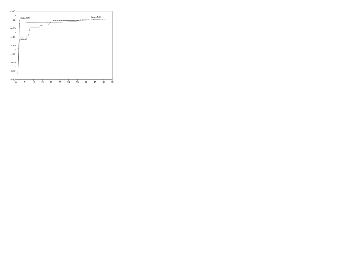
Figure 1: Evolution of the log-likelihood versus iteration number: MCL Female CR case

Figure 2: Evolution of the log-likelihood versus iteration number: MCL Male AL case

Figure 3: Evolution of the log-likelihood versus iteration number: Detail of MCL Male AL case

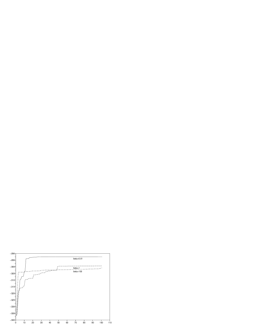
Figure 4: Evolution of the log-likelihood versus iteration number: MCL Female AL case

6 Conclusions

The goal of this paper was the study of the asymptotic behavior of the EM algorithm and its proximal generalizations. We clarified the analysis by making use of the Kullback-proximal theoretical framework. Two of our main contributions are the following. Firstly we showed that interior cluster points are stationary points of the likelihood function and are local maximizers for sufficiently small values of $\beta$. Secondly, we showed that cluster points lying on the boundary satisfy the Karush-Kuhn-Tucker conditions. Such cases were very seldom studied in the literature although constrained estimation is a topic of growing importance; see for instance the special issue of the Journal of Statistical Planning and Inference [10] which is devoted to the problem of estimation under constraints. On the negative side, the analysis from the Kullback-proximal viewpoint allowed us to understand why uniqueness of the cluster point is hard to establish theoretically. On the positive side, we were able to implement a new and efficient proximal point method for estimation in the difficult tumor lethality problem involving nonlinear inequality constraints.

References

- [1] H. Ahn, H. Moon and R.L. Kodell, ”Attribution of tumour lethality and estimation of the time to onset of occult tumours in the absence of cause-of-death information”. J. Roy. Statist. Soc. Ser. C, vol. 49, no. 2, 157–169, 2000.
- [2] M.J. Box, ”A new method of constrained optimization and a comparison with other methods”, The Computer Journal, 8, 42–52, 1965.
- [3] G. Celeux, S. Chretien, F. Forbes and A. Mkhadri, ”A component-wise EM algorithm for mixtures”, J. Comput. Graph. Statist. 10 (2001), no. 4, 697–712 and INRIA RR-3746, Aug. 1999.
- [4] S. Chretien and A.O. Hero, ”Acceleration of the EM algorithm via proximal point iterations”, Proceedings of the International Symposium on Information Theory, MIT, Cambridge, p. 444, 1998.
- [5] S. Chrétien and A. Hero, “Kullback proximal algorithms for maximum-likelihood estimation,” IEEE Trans. Inform. Theory 46 (2000), no. 5, 1800–1810.
- [6] T. Cover and J. Thomas, Elements of Information Theory, Wiley, New York, 1987.
- [7] I. Csiszár, ”Information-type measures of divergence of probability distributions and indirect observations”, Studia Sci. Math. Hung., 2 (1967), 299–318.
- [8] A. P. Dempster, N. M. Laird, and D. B. Rubin, “Maximum likelihood from incomplete data via the EM algorithm,” J. Royal Statistical Society, Ser. B, vol. 39, no. 1, pp. 1–38, 1977.
- [9] I. A. Ibragimov and R. Z. Has’minskii, Statistical estimation: Asymptotic theory, Springer-Verlag, New York, 1981.
- [10] Journal of Statistical Planning and Inference, vol. 107, no. 1–2, 2002.
- [11] A. T. Kalai and S. Vempala “Simulated annealing for convex optimization”. Math. Oper. Res. 31 (2006), no. 2, 253–266.
- [12] K. Lange and R. Carson, “EM reconstruction algorithms for emission and transmission tomography,” Journal of Computer Assisted Tomography, vol. 8, no. 2, pp. 306–316, 1984.
- [13] B. Martinet, “Régularisation d’inéquation variationnelles par approximations successives,” Revue Francaise d’Informatique et de Recherche Operationnelle, vol. 3, pp. 154–179, 1970.
- [14] G.J. McLachlan and T. Krishnan, “The EM algorithm and extensions,” Wiley Series in Probability and Statistics: Applied Probability and Statistics. John Wiley and Sons, Inc., New York, 1997.
- [15] H. Moon, H. Ahn, R. Kodell and B. Pearce ” A comparison of a mixture likelihood method and the EM algorithm for an estimation problme in animal carcinogenicity studies,” Computational Statistics and Data Analysis, 31 , no. 2, pp. 227–238, 1999.
- [16] A. M. Ostrowski Solution of equations and systems of equations. Pure and Applied Mathematics, Vol. IX. Academic Press, New York-London 1966
- [17] R. T. Rockafellar, “Monotone operators and the proximal point algorithm,” SIAM Journal on Control and Optimization, vol. 14, pp. 877–898, 1976.
- [18] L. A. Shepp and Y. Vardi, “Maximum likelihood reconstruction for emission tomography,” IEEE Trans. on Medical Imaging, vol. MI-1, No. 2, pp. 113–122, Oct. 1982.
- [19] M. Teboulle, “Entropic proximal mappings with application to nonlinear programming,” Mathematics of Operations Research, vol. 17, pp. 670–690, 1992.
- [20] P. Tseng, “An analysis of the EM algorithm and entropy-like proximal point methods,” Mathematics of Operations Research, vol. 29, pp. 27–44, 2004.
- [21] C. F. J. Wu, “On the convergence properties of the EM algorithm,” Annals of Statistics, vol. 11, pp. 95–103, 1983.
- [22] Z. B. Zabinsky “Stochastic adaptive search for global optimization”. Nonconvex Optimization and its Applications, 72. Kluwer Academic Publishers, Boston, MA, 2003.
- [23] W. I. Zangwill and B. Mond, Nonlinear programming: a unified approach, Prentice-Hall International Series in Management. Prentice-Hall, Inc., Englewood Cliffs, N.J., 1969.