Entropy Production in Collisionless Systems. II. Arbitrary Phase-Space Occupation Numbers

Abstract

We present an analysis of two thermodynamic techniques for determining equilibria of self-gravitating systems. One is the Lynden-Bell entropy maximization analysis that introduced violent relaxation. Since we do not use the Stirling approximation which is invalid at small occupation numbers, our systems have finite mass, unlike Lynden-Bell’s isothermal spheres. (Instead of Stirling, we utilize a very accurate smooth approximation for $\ln{x!}$.) The second analysis extends entropy production extremization to self-gravitating systems, also without the use of the Stirling approximation. In addition to the Lynden-Bell (LB) statistical family characterized by the exclusion principle in phase-space, and designed to treat collisionless systems, we also apply the two approaches to the Maxwell-Boltzmann (MB) families, which have no exclusion principle and hence represent collisional systems. We implicitly assume that all of the phase-space is equally accessible. We derive entropy production expressions for both families, and give the extremum conditions for entropy production. Surprisingly, our analysis indicates that extremizing entropy production rate results in systems that have maximum entropy, in both LB and MB statistics. In other words, both thermodynamic approaches lead to the same equilibrium structures.

1. Introduction

1.1. Motivation

Understanding how collisionless systems attain a specific mechanical equilibrium state is fundamentally important to astrophysics. For example, the cold dark matter structures that exist around galaxies are expected to fall into this class of system. Individual dark matter constituents (whatever they may be) should evolve according to a mean-field gravitational potential, free of the influence of individual encounters.

The range of mechanical equilibria available to a collisionless system is defined by the Jeans equation, which represents the condition that no portion of the system experiences a net force. Unfortunately, the Jeans equation admits an infinity of solutions. Even if the mass distribution is specified, there is an infinite set of acceptable mechanical equilibria, each involving a different velocity distribution. For spherical systems, these velocity distributions differ in their anisotropy profile that quantifies radial versus tangential motion. However, the question remains, how and/or why does any one collisionless system evolve to its particular mechanical equilibrium end-state, and what are the properties of such a state?

1.2. Thermodynamic Approaches to the Problem

The statistical mechanics description of thermodynamics provides one path to obtaining the description of the final relaxed state. A fully relaxed system is the most statistically likely state of that system, or the one with an entropy maximum. In calculating the most likely state it is implicitly assumed that all states of the system are equally accessible.

Such an approach was taken by Lynden-Bell (1967) and applied to self-gravitating collisionless systems, with the hope of explaining the observed light distribution of elliptical galaxies. A collisionless system can be thought of as a fluid in the 6D phase-space of position and velocity. The ‘particles’ in Lynden-Bell’s analysis are parcels of phase-space, i.e., parcels of this fluid, and so the distribution function (DF) representing the phase-space density is defined in terms of energy per unit mass, not energy per particle. The analysis resulted in a DF similar to the Fermi-Dirac case, but with a different normalization. Lynden-Bell (1967) argued that a non-degenerate limit is appropriate for stellar systems, and thus arrived at a DF similar to that of the Maxwell-Boltzmann case (an exponential) which resulted in the isothermal sphere representing thermal equilibrium. Since the isothermal sphere has an infinite extent and mass, its emergence from the entropy maximization procedure, which demanded a finite mass system, presented a contradiction. This apparent failure of entropy maximization was puzzling, and it was often argued that such systems do not have states of maximum entropy. Some effort was made to investigate maximizing entropy with additional constraints beyond mass, energy, and angular momentum (Stiavelli & Bertin, 1987; White & Narayan, 1987). Other routes involving minimum energy states of self-gravitating systems were also developed (e.g., Aly, 1994).

Recently, Madsen (1996) (based on earlier work by Simons, 1994) has pointed out that the reason for the system’s infinite mass was the use of the Stirling approximation, $\ln{n!}\approx n\ln{n}-n$. In contrast to systems usually treated in standard statistical mechanics, self-gravitating systems can apparently have small phase-space occupation numbers $n$, making Stirling a poor approximation. Specifically, these systems have regions of phase-space or energy-space that are nearly or completely unoccupied, such that $n$ will be small. Spatially, these regions can correspond to the center of the potential as well as its outer edge. Using Maxwell-Boltzmann statistics and the exact $\ln{n!}$, Madsen (1996) has found a distribution function from entropy maximization that is very similar to King (1966) models. Hjorth & Williams (2010) have shown that the energy-space occupation function $N(E)$ derived using a very accurate smooth approximation to $\ln{n!}$ closely resembles the results of collisionless $N$-body simulations (Williams et al., 2010).

1.3. Brief Review of Statistical Representations

From a statistical point of view, entropy is simply a measurement of the number of states accessible to a particular system. This relationship is most commonly expressed quantitatively as,

$$S=k_{\rm B}\ln{\Omega},$$ (1)

where $\Omega$ is the number of accessible states and $k_{\rm B}$ is the Boltzmann constant which serves to give entropy the correct thermodynamic units. As a result, counting procedures are key to determining specific realizations of entropy. Lynden-Bell (1967) discusses how there are four counting types that lead to physically relevant situations. Bose-Einstein statistics follow from counting states for indistinguishable particles that can co-habitate in the same state. When indistinguishable particles are not allowed to share states, Fermi-Dirac (FD) statistics emerge. Classical Maxwell-Boltzmann (MB) statistics result from counting states available to distinguishable particles that can share states. Completing the symmetry, systems where distinguishable ‘particles’—actually, parcels of phase-space—cannot co-occupy states obey what has become known as Lynden-Bell (LB) statistics (statistics ‘IV’ in Lynden-Bell’s original notation). Each type of statistics will produce different representations of entropy, but we will focus on the two that deal with classical, or distinguishable particles, namely, LB and MB.

We briefly recap the notation used in Lynden-Bell (1967) before proceeding with our discussion. The six-dimensional position-velocity phase-space ($\boldsymbol{x}$,$\boldsymbol{v}$) is the usual setting for determining the statistics. Imagine phase-space to be divided into a very large number of nearly infinitesimal parcels, called micro-cells, each having volume $\varpi$. Each micro-cell can either be occupied or unoccupied by one of the $N$ phase-space elements of the system. These elements can be thought of as representing the fine-grained distribution function, which has a constant density value $\eta$. Because collisionless processes imply incompressibility of the fine-grained distribution function, the phase elements cannot co-habitate. If phase-space is also partitioned on a coarser level so that some number $\nu$ of micro-cells occupy a macro-cell, then we can discuss a coarse-grained distribution function. The volume of a macro-cell is then $\nu\varpi$ and the $i$th macro-cell contains $n_{i}$ phase elements. We assume that while the volume of a macro-cell is much larger than that of a micro-cell, it is still very small compared to the full extent of phase-space occupied by the system. The number of ways of organizing the $n_{i}$ elements into the $\nu$ micro-cells without co-habitation is,

$$\frac{\nu!}{(\nu-n_{i})!}.$$ (2)

If the elements were allowed to multiply occupy micro-cells, as in MB statistics, this number would be given by $\nu^{n_{i}}$.

To get the total number of accessible states, the possible ways to distribute the $N$ phase elements into $n_{i}$ chunks must also be included. Lynden-Bell (1967) derives,

$$\Omega_{\rm LB}=\frac{N!}{\prod_{i}n_{i}!}\times\prod_{i}\frac{\nu!}{(\nu-n_{i})!}.$$ (3)

In the MB case, the only change is that the factorial ratio in the final product term is replaced by $\nu^{n_{i}}$.

The LB case disallows two phase-space elements from inhabiting the same phase-space location, so it explicitly takes into account the incompressibility of a collisionless fluid. Since we are primarily interested in dark matter halos, LB is the natural case to consider. For completeness, and for the sake of having a comparison, we also treat the MB case, in the Appendix.

We argue that the lack of an exclusion principle in the MB case is equivalent to allowing collisions between particles. In a collisional system, particles from distant phase-space locations can be scattered into any other phase-space location, thereby increasing the phase-space density at the latter location. In principle, there is no limit to how high the density can get through such scatterings. In practice, the phase-space density probably can not become very high at most locations, but it can be higher than the original fine-grained DF. We note that it is common to use MB to represent collisional systems. For example, Madsen (1996) argues that it is the correct statistics to use for globular clusters where the relatively small number of stars allows the cluster to relax through two-body interactions. It then makes sense that the energy distribution that the cluster will arrive at will be the same as that in a cloud of gas, which relaxes through collisions between molecules. In the non-degenerate limit, when the micro-cells are very sparsely populated and the density of the coarse-grained distribution function is very dilute compared to that of the fine-grained function, both LB and MB distribution functions, and hence density profiles, will look the same.

1.4. This Work

In this paper we explore two possible approaches to deriving the final equilibrium state of self-gravitating systems, for each of the two types of statistics, LB and MB. In both, we use a very accurate, smooth approximation for $\ln{x!}$ valid for arbitrary occupation numbers $x$. However, the price we pay for this improved approximation is the loss of analytic solutions.

The first approach assumes that the final state is the maximum entropy state, an assumption that was first used in the context of self-gravitating systems in 1950’s (Ogorodnikov, 1957). The second approach, again in the context of self-gravitating systems, was first taken by Barnes & Williams (2011); it posits that the final state corresponds to the extremum of entropy production rate.

We explore extremizing entropy production because it has not been established beyond a doubt that real or computer simulated systems do fully relax to maximum entropy states. It is possible that their steady-state configurations do not correspond to maximum entropy. Prior work on thermal non-equilibrium systems, but not in astrophysical contexts, suggests that stationary states—like mechanical equilibrium—occur when entropy production is extremized (e.g., Prigogine, 1961; Jaynes, 1980; de Groot & Mazur, 1984; Grandy, 2008). We investigate their applicability to self-gravitating systems in mechanical equilibrium.

The new aspect in the present paper is that we use a very accurate approximation for $\ln{x!}$, unlike our previous paper that assumed the Stirling approximation. As Madsen (1996) has shown, replacing Stirling with an accurate approximation (i) results in systems with finite total mass and energy, and (ii) significantly changes the structure of the systems.

In all, we present four derivations; entropy maximization for the LB and MB statistics are covered in Sections 3.1 and  A.1. Extremization of entropy production for LB and MB statistics are carried out in Sections 3.2 and  A.2, respectively. We develop expressions for the relaxation functions (see § 2), and use these to better understand the evolution of coarse-grained distribution function. We compare our results with analogous versions of entropy production derived using the standard Stirling approximation in Barnes & Williams (2011).

Figure 1 puts the present paper (BWII in the figure) in context. It is a schematic summary of the various statistical mechanical approaches to self-gravitating systems. The possible ways to frame the problem appears at the top of the figure; one can formulate the problem in either the regular phase-space, or the energy space. Below the thick horizontal line we show the two different routes for attaining the final steady-state state: maximizing entropy, and extremizing entropy production. Once these choices are made one has to decide whether small occupation number regime will be important or not, and hence whether to use the Stirling approximation for $\ln x!$, or not. In the latter case, one must then decide whether to use the discrete (“discr.”) step-like, i.e. exact version of $\ln x!$, or to approximate it with some smooth function (“cont.”) which remains very accurate down to small $x$. Note that HW10 and the present paper use different but similar approximations. There is no physical reason to introduce the exclusion principle in the energy state-space, hence the corresponding regions are marked as “not relevant”. The bottom entries of some columns in the table contain names of papers where the corresponding options were considered. K66 in parentheses below BWII means that King (1966) results are nearly identical to ours. $M=\infty$ under LB67 means that Lynden-Bell (1967) final result, the isothermal sphere, had infinite mass.

Much of the background material for this work may be found in Barnes & Williams (2011), and we briefly summarize these previously obtained results in Section 2.

2. Summary of Results for Large Occupation Numbers

Barnes & Williams (2011) have investigated entropy production in self-gravitating systems described by MB and LB and have developed expressions for the entropy production, $\sigma$ for both the MB,

$$\sigma_{\rm MB}=-\frac{k_{\rm B}}{\varpi\eta}\int\Gamma\left[\ln{\left(\frac{f}{\eta}\right)}+1-\ln{N}\right]\>\mathrm{d}\boldsymbol{v},$$ (4)

and LB cases,

$$\sigma_{\rm LB}=-\frac{k_{\rm B}}{\varpi\eta}\int\Gamma\left[\ln{\left(\frac{f}{\eta-f}\right)}-C\right]\>\mathrm{d}\boldsymbol{v},$$ (5)

where constant $C$ in Equation 5 is $(\ln{N}-1)+(1/N)\sum_{i}\nu\ln{\nu}$. In these expressions, $f$ is the coarse-grained distribution function and $\Gamma$ is the relaxation function and forms the right-hand side of the Boltzmann equation,

$$\frac{\partial f}{\partial t}+\boldsymbol{v}\boldsymbol{\cdot}\boldsymbol{\nabla}f+\boldsymbol{a}\boldsymbol{\cdot}\boldsymbol{\nabla}_{v}f=\Gamma(f).$$ (6)

If one were to assume, for a moment, that in the above equation $f$ is a fine-grained DF, then the right hand side would be zero for collisionless systems. In other words $\Gamma=0$, which means that on fine-grained scales there is no change in, or production of entropy; in collisionless systems, entropy is fixed throughout evolution. Let us be clear, we are not advocating for a specific process as a source for $\Gamma$, like collisions in a gas. The relaxation function simply describes the Lagrangian time rate of change of the distribution function. Returning to our case where $f$ represents the coarse-grained DF, Equation 6 states that entropy is produced [and as we argue in Barnes & Williams (2011) it happens even in systems that have attained macroscopic steady-state] because on microscopic scales the fine-grained DF continues to wind and twist, which when combined with coarse-graining, gives rise to non-zero entropy change. From a different starting point, Chavanis (1998) develops an expression for the right-hand side of Equation 6 in terms of a “diffusion current” that relates to correlations between fluctuations in the fine-grained distribution function. While that work details the makeup of this diffusion current, we simply focus on the broad behavior of the relaxation function.

We find extremum entropy production conditions by setting the variation of entropy production, $\delta\sigma$ equal to zero. This operation gives expressions for the relaxation function. For the MB case,

$$\Gamma_{\rm MB}(f)=\frac{(1-\ln{N})\Gamma_{\rm MB}(f=\eta)}{\ln{(f/\eta)}+1-\ln{N}}.$$ (7)

The LB relaxation function is slightly more complex,

$$\Gamma_{\rm LB}(f)=\frac{-C\Gamma_{\rm LB}(f=\eta/2)}{\ln{[f/(\eta-f)]}-C}.$$ (8)

Like Lynden-Bell (1967), the Barnes & Williams (2011) work assumes that the large $n$ Stirling approximation is valid for the systems being investigated. Here, we will be deriving relations analogous to Equations 4, 5, 7, and 8, but using a very accurate approximation, after discussing the results of entropy maximization below.

3. Results for Arbitrary Occupation Numbers

The approximation that we utilize in this work is,

$$\ln{x!}=(x+\frac{1}{2})\ln{(x+1)}-x+\frac{\ln{2\pi}}{2}+\lambda_{0,x}$$ (9)

where

$$\lambda_{0,x}=-\frac{(x^{2}+2x+\frac{287}{288})}{(x^{2}+\frac{25}{12}x+\frac{13}{12})}.$$ (10)

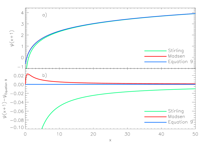
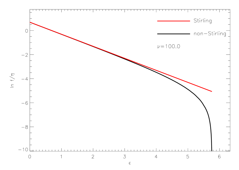
In the large $x$ limit, this reduces to the usual Stirling approximation $\ln{x!}=x\ln{x}-x$. Our approximation is slightly different from the one in Hjorth & Williams (2010). Comparisons between the Stirling approximation, Hjorth & Williams (2010) approximation, and Equation 9 are shown in Figure 2. The plots illustrate the function $\psi(x+1)\equiv\mathrm{d}\ln{x!}/\mathrm{d}x$ for the three cases. The HW10 and Equation 9 approximations are nearly identical. Most importantly, these two approximations are well-behaved at $x=0$, unlike the Stirling approximation.

3.1. Entropy Maximization

In this section, we follow the overall path taken in Lynden-Bell (1967) to determine the description of entropy for the LB statistics family. Briefly, counting arguments for phase-space macro-cell occupation are combined with the statistical definition of entropy to give specific representations. Variations in entropy assuming constant mass and energy are then set to zero in order to determine the necessary distribution functions.

If one demands that multiple phase-space elements cannot simultaneously occupy micro-cells, the multiplicity of states (Equation 3) combined with the definition of entropy results in,

$$S_{\rm LB}=k_{\rm B}\left[\ln{N!}-\sum_{i}\ln{n_{i}!}+\sum_{i}\ln{\nu!}-\sum_{i}\ln{(\nu-n_{i})!}\right],$$ (11)

where again the summations run over the number of macro-cells. We will assume that both $N$ and $\nu$ are much larger than 1, so that Stirling’s approximation is valid for use in the first and third terms. However, for the $n_{i}$ and $\nu-n_{i}$ terms we will use our improved approximation,

$$\ln{n_{i}!}=(n_{i}+1/2)\ln{(n_{i}+1)}-n_{i}+\frac{\ln{2\pi}}{2}+\lambda_{0,n_{i}}.$$ (12)

Note that this usage does not require either $n_{i}$ or $\nu-n_{i}$ to actually be a small value, rather this keeps the accounting accurate in the event that they do become small. If these values are always large, there will be no difference from the Stirling approximation. The entropy expression now reads,

$$S_{\rm LB} = S_{\rm LB,0}-k_{\rm B}\sum_{i}\left[(n_{i}+1/2)\ln{(n_{i}+1)}+\right.$$ (13)

$$(\nu-n_{i}+1/2)\ln{(\nu-n_{i}+1)}+\lambda_{0,n_{i}}+$$

$$\left.\lambda_{0,(\nu-n_{i})}\right],$$

where $S_{\rm LB,0}=k_{\rm B}[N\ln{N}-N+M(\nu\ln{\nu}-\ln{2\pi})]$, and $M$ is the total number of macro-cells.

Transforming from the discrete macro-cell occupation number $n_{i}$ to the continuous coarse-grained distribution function $f$, the entropy becomes,

$$S_{\rm LB} = S_{\rm LB,0}-\frac{k_{\rm B}}{\nu\varpi}\iint\left[\left(\frac{\nu f}{\eta}+\frac{1}{2}\right)\ln{\left(\frac{\nu f}{\eta}+1\right)}+\right.$$ (14)

$$\left(\nu-\frac{\nu f}{\eta}+\frac{1}{2}\right)\ln{\left(\nu-\frac{\nu f}{\eta}+1\right)}+\lambda_{0,\nu f/\eta}+$$

$$\left.\lambda_{0,\nu-\nu f/\eta}\right]\>\mathrm{d}\boldsymbol{x}\>\mathrm{d}\boldsymbol{v}.$$

Taking the variation of this entropy expression to be zero, with constant mass and energy constraints, leads to the following condition,

$$\ln{(F+1)}+\frac{(F+1/2)}{(F+1)}-\ln{(\nu-F+1)}-$$ (15)

$$\frac{(\nu-F+1/2)}{(\nu-F+1)}+$$

$$\frac{\mathrm{d}\lambda_{0,F}}{\mathrm{d}F}+\frac{\mathrm{d}\lambda_{0,\nu-F}}{\mathrm{d}F}+\mu+\beta\epsilon=0,$$

where $F=\nu f/\eta$ is a scaled coarse-grained distribution function and $\mu$ and $\beta$ are undetermined multipliers associated with mass and energy conservation, respectively. The $\epsilon$ term is the specific energy of a phase element located at position $\boldsymbol{x}$ with velocity $\boldsymbol{v}$, $\epsilon=v^{2}/2+\Phi$. The derivative of the $\lambda$ function is,

$$\frac{\mathrm{d}\lambda_{0,F}}{\mathrm{d}F}=\frac{-(F+1)}{(F+600/576)}.$$ (16)

After substituting for these $\lambda$ derivatives and combining terms we have,

$$\ln{\left[\frac{F+1}{\nu-F+1}\right]}+\frac{(F-\nu/2)}{(F+1)(\nu-F+1)}-$$ (17)

$$\frac{2F^{2}-2F\nu-(1+600/576)\nu-600/288}{F^{2}-F\nu-(600/576)\nu+(600/576)^{2}}+$$

$$\mu+\beta\epsilon=0.$$

The inelegant ratio terms in this expression are both symmetric about $F=\nu/2$. The second term on the left-hand side of Equation 17 has values of $-1/2$ when $F=0$, $0$ when $F=\nu/2$, and $1/2$ when $F=\nu$ (the maximum value of $F$ for the LB case). The third term on the left-hand side of Equation 17 is a nearly constant function with a value very close to $-2$ for $0\leq F\leq\nu$.

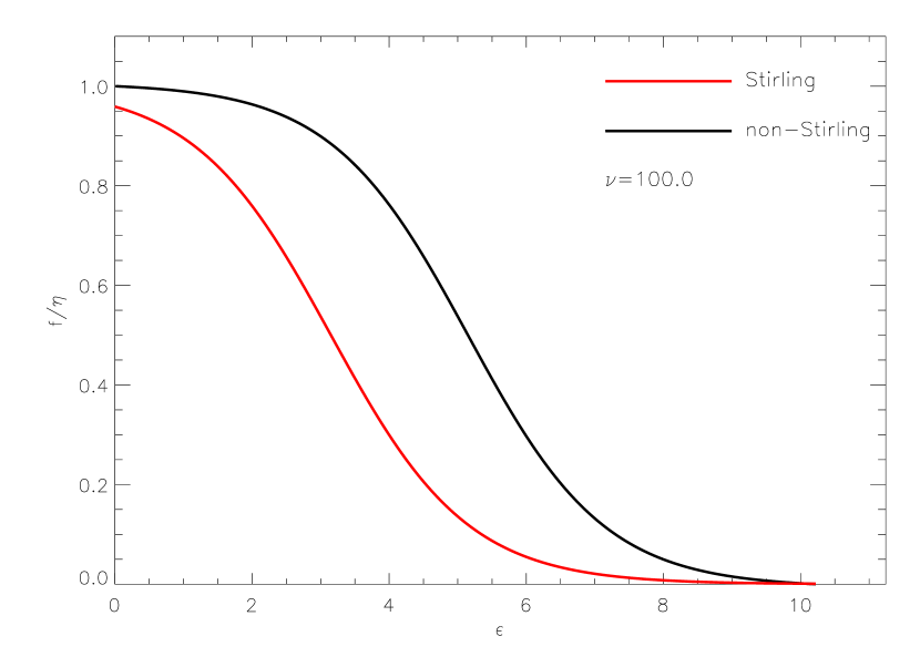
We have not attempted to find an analytic solution for $F$. Graphical solutions of Equation 17 for a series of $\epsilon$ values produces the picture of $f/\eta$ seen in Figure 3. The overall character of the distribution function is the same in the non-Stirling and Stirling versions, and both functions are very similar to Fermi-Dirac distribution,

$$f_{\rm FD}=\frac{\exp{-(\mu+\beta\epsilon)}}{1+\exp{-(\mu+\beta\epsilon)}}.$$ (18)

This distribution function of Equation 17 can be transformed into a density distribution using the Poisson equation and the fact that

$$\rho(r)=\int f(r,v)\mathrm{d}\boldsymbol{v}=4\pi\int f(\epsilon)\sqrt{2[\epsilon-\Phi(r)]}\mathrm{d}\epsilon.$$ (19)

Note that this procedure imposes an isotropic velocity distribution for the system.

The density and logarithmic density slope corresponding to the non-Stirling function are presented in Figures 4 and 5, and will be discussed further in Section 4.1.

3.2. Entropy Production Extremization

Just because it is possible to describe thermal equilibrium states for collisionless self-gravitating systems, it does not follow that real systems (either physical or simulated) must achieve them in a Hubble time. It is possible that real systems incompletely relax, leaving them in a thermal non-equilibrium, but long-lived stationary state. Madsen (1996) also points out that in very slowly evolving systems, the maximization of entropy is only temporary. This leads us to infer that the production of entropy may be a useful quantity for discussing quasi-equilibria of collisionless systems. With that in mind, we now proceed to develop the conditions required for a thermal non-equilibrium state to be stationary. Specifically, we find an expression for entropy production in the LB statistical family and then extremize it. (As for the preceding section, an analogous derivation for the Maxwell-Boltzmann statistics may be found in Appendix A.2.) As discussed in Section 1.4, existing work on thermal non-equilibrium in non-astrophysical settings suggests that stationary states occur when entropy production is either maximum or minimum (de Groot & Mazur, 1984; Grandy, 2008, and references therein).

From Equation 14 the entropy density in the Lynden-Bell case can be written as,

$$\rho s_{\rm LB}=-\frac{k_{\rm B}}{\nu\varpi}\int\Bigg{[}(F+1/2)\ln{(F+1)}-$$ (20)

$$(\nu-F+1/2)\ln{(\nu-F+1)}+$$

$$\lambda_{0,F}+\lambda_{0,\nu-F}-F\frac{S_{\rm LB,0}}{Nk_{\rm B}}\Bigg{]}\>\mathrm{d}\boldsymbol{v},$$

where, as before, $F\equiv\nu f/\eta$.

Taking a partial time derivative of Equation 20 results in

$$\frac{\partial}{\partial t}(\rho s_{\rm LB})=-\frac{k_{\rm B}}{\nu\varpi}\int\frac{\partial F}{\partial t}\left[\ln{(F+1)}+\right.$$ (21)

$$\frac{F+1/2}{F+1}-\ln{(\nu-F+1)}+\frac{\nu-F+1/2}{\nu-F+1}+$$

$$\left.\frac{\partial\lambda_{0,F}}{\partial F}+\frac{\partial\lambda_{0,\nu-F}}{\partial F}-C\right]\>\mathrm{d}\boldsymbol{v},$$

where $C=S_{\rm LB,0}/Nk_{\rm B}$ is a constant.

Upon substituting $\partial F/\partial t$ from the Boltzmann equation into Equation 21, we get a lengthy expression,

$$\frac{\partial}{\partial t}(\rho s_{\rm LB})=$$ (22)

$$-\frac{k_{\rm B}}{\nu\varpi}\int(-\boldsymbol{v}\boldsymbol{\cdot}\boldsymbol{\nabla}F)\Bigg{[}\ln{(F+1)}+\frac{(F+1/2)}{(F+1)}-$$

$$\ln{(\nu-F+1)}+\frac{\nu-F+1/2}{\nu-F+1}+\frac{\partial\lambda_{0,F}}{\partial F}+\frac{\partial\lambda_{0,\nu-F}}{\partial F}-C\Bigg{]}\>\mathrm{d}\boldsymbol{v}-$$

$$\frac{k_{\rm B}}{\nu\varpi}\int(-\boldsymbol{a}\boldsymbol{\cdot}\boldsymbol{\nabla}_{v}F)\Bigg{[}\ln{(F+1)}+\frac{(F+1/2)}{(F+1)}-$$

$$\ln{(\nu-F+1)}+\frac{\nu-F+1/2}{\nu-F+1}+\frac{\partial\lambda_{0,F}}{\partial F}+\frac{\partial\lambda_{0,\nu-F}}{\partial F}-C\Bigg{]}\>\mathrm{d}\boldsymbol{v}-$$

$$\frac{k_{\rm B}}{\nu\varpi}\int\gamma\Bigg{[}\ln{(F+1)}+\frac{(F+1/2)}{(F+1)}-$$

$$\ln{(\nu-F+1)}+\frac{\nu-F+1/2}{\nu-F+1}+\frac{\partial\lambda_{0,F}}{\partial F}+$$

$$\frac{\partial\lambda_{0,\nu-F}}{\partial F}-C\Bigg{]}\>\mathrm{d}\boldsymbol{v},$$

where $\gamma=\nu\Gamma/\eta$.

The first term on the right-hand side of Equation 22 can be transformed into $-\boldsymbol{\nabla}\boldsymbol{\cdot}\rho s_{\rm LB}\boldsymbol{v}$. The acceleration-dependent terms in Equation 22 all disappear under the assumptions that the distribution function is even in $v$ and disappears when $v=v_{\rm max}$. The final representation of the time rate of change of the entropy density is,

$$\frac{\partial}{\partial t}(\rho s_{\rm LB})=$$ (23)

$$-\frac{k_{\rm B}}{\nu\varpi}\boldsymbol{\nabla}\boldsymbol{\cdot}\int[(F+1/2)\ln{(F+1)}-$$

$$(\nu-F+1/2)\ln{(\nu-F+1)}+\lambda_{0,F}+\lambda_{0,\nu-F}-FC]\boldsymbol{v}\>\mathrm{d}\boldsymbol{v}-$$

$$\frac{k_{\rm B}}{\nu\varpi}\int\gamma(F)\Bigg{[}\ln{(F+1)}+\frac{F+1/2}{F+1}-\ln{(\nu-F+1)}+$$

$$\frac{\nu-F+1/2}{\nu-F+1}+\frac{\mathrm{d}\lambda_{0,F}}{\mathrm{d}F}+\frac{\mathrm{d}\lambda_{0,\nu-F}}{\mathrm{d}F}-C\Bigg{]}\>\mathrm{d}\boldsymbol{v}.$$

Again assuming the velocity field to be composed of mean and peculiar components $\boldsymbol{v}=\boldsymbol{v_{0}}+\boldsymbol{v_{p}}$, we draw a correspondence between the terms in,

$$\frac{\partial}{\partial t}(\rho s_{\rm LB})=-\boldsymbol{\nabla}\boldsymbol{\cdot}\rho s_{\rm LB}\boldsymbol{v_{0}}-$$ (24)

$$\frac{k_{\rm B}}{\nu\varpi}\boldsymbol{\nabla}\boldsymbol{\cdot}\int[(F+1/2)\ln{(F+1)}-$$

$$(\nu-F+1/2)\ln{(\nu-F+1)}+\lambda_{0,F}+\lambda_{0,\nu-F}-FC]\boldsymbol{v_{p}}\>\mathrm{d}\boldsymbol{v}-$$

$$\frac{k_{\rm B}}{\nu\varpi}\int\gamma\Bigg{[}\ln{(F+1)}+\frac{F+1/2}{F+1}-\ln{(\nu-F+1)}+$$

$$\frac{\nu-F+1/2}{\nu-F+1}+\frac{\mathrm{d}\lambda_{0,F}}{\mathrm{d}F}+\frac{\mathrm{d}\lambda_{0,\nu-F}}{\mathrm{d}F}-C\Bigg{]}\>\mathrm{d}\boldsymbol{v}.$$

and those in the continuous version of the entropy density evolution equation, (Equation 6 in Barnes & Williams, 2011),

$$\frac{\partial}{\partial t}(\rho s)=-\boldsymbol{\nabla}\boldsymbol{\cdot}(\boldsymbol{\Sigma}+\rho s\boldsymbol{v_{0}})+\sigma.$$ (25)

The entropy flux due to random motions $\boldsymbol{\Sigma}$ is given by the integral in the second term on the right-hand side of Equation 24. The remaining term then makes up the entropy production for the system,

$$\sigma_{\rm LB} = -\frac{k_{\rm B}}{\nu\varpi}\int\gamma\Bigg{[}\ln{(F+1)}+\frac{F+1/2}{F+1}-\ln{(\nu-F+1)}+$$ (26)

$$\frac{\nu-F+1/2}{\nu-F+1}+\frac{\mathrm{d}\lambda_{0,F}}{\mathrm{d}F}+\frac{\mathrm{d}\lambda_{0,\nu-F}}{\mathrm{d}F}-C\Bigg{]}\>\mathrm{d}\boldsymbol{v}.$$

As expected, the relaxation function determines the entropy production rate for the system.

We find that the condition for the entropy production term in Equation 26 to be extremized is,

$$\Gamma_{\rm LB}(f)=Q/\left[\ln{\left(\frac{F+1}{\nu-F+1}\right)}+\frac{F+1/2}{F+1}+\right.$$ (27)

$$\left.\frac{\nu-F+1/2}{\nu-F+1}+\frac{\mathrm{d}\lambda_{0,F}}{\mathrm{d}F}+\frac{\mathrm{d}\lambda_{0,\nu-F}}{\mathrm{d}F}-C\right],$$

where the integration constant is defined by,

$$Q=\gamma_{\rm LB}(F=\nu/2)\left[\frac{\nu+1}{\nu/2+1}-\frac{2(\nu+2)}{\nu+600/288}-C\right],$$ (28)

and the $\lambda$ derivatives are the same as those used in going from Equation 15 to 17. This relaxation function is shown in Figure 7 and is very similar to the corresponding function from Barnes & Williams (2011), their Figure 2.

4. Summary and Discussion

In an attempt to better understand the evolution of self-gravitating collisionless systems, we have re-investigated a standard statistical mechanics approach to finding equilibria (entropy maximization), and continued to develop a new approach (extremization of entropy production), first applied to self-gravitating systems by Barnes & Williams (2011). Entropy production in non-equilibrium steady-state systems has been previously investigated and found to be useful in several non-astrophysical systems, and so it is interesting to ask if the principle is relevant in gravitational systems.

Both of our approaches use a very accurate approximation for $\ln n!$, and not the standard Stirling formula valid only for large occupation numbers. It has been recently shown that using an approximation that reflects correct behavior for small $n$, and the principle of entropy maximization leads to density distributions that resemble globular clusters (King profiles; Madsen, 1996), and simulated pure dark matter halos (Williams & Hjorth, 2010; Williams et al., 2010). Both types of systems have finite mass and energy, in compliance with the entropy maximization constraints.

4.1. Results of Entropy Maximization

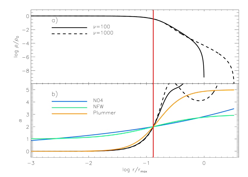
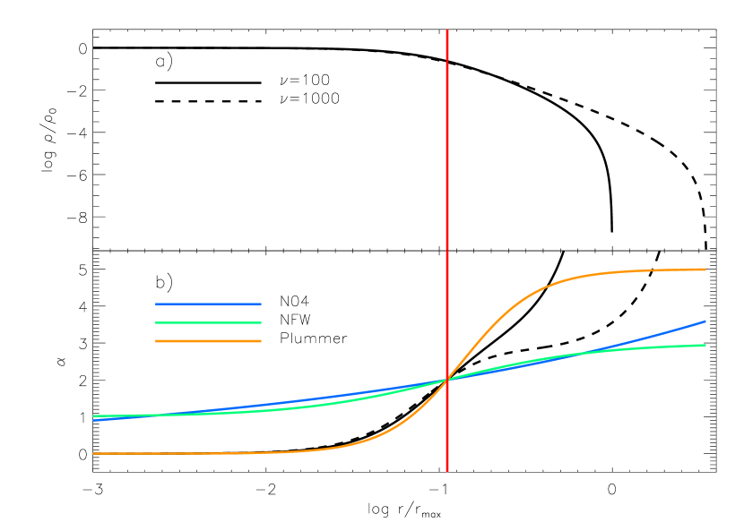
Entropy maximization using the LB and MB statistics produces the density profiles and logarithmic profiles slopes, $\alpha=-\mathrm{d}\log{\rho}/\mathrm{d}\log{r}$ depicted in Figures 4 and 9, respectively.

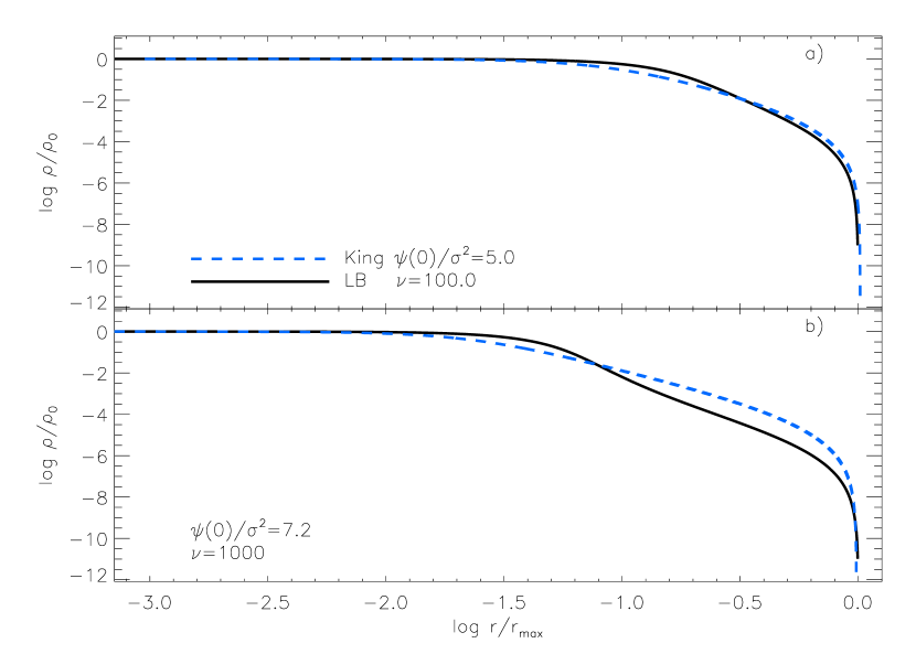
We argue that the LB case accurately represents collisionless systems because co-habitation of the phase-space elements is prohibited. However, the density profiles for any value of $\nu$ is very different from the two cosmological models, Navarro-Frenk-White (NFW) (Navarro et al., 1996) and N04 (Navarro et al., 2004), which are fits to the results of cosmological $N$-body simulations. In contrast to the latter, the LB density profiles have a flat central density slope, while at larger radii $\alpha$ has a steeper rise than even that of the Plummer profile (Schuster, 1883; Plummer, 1911; Binney & Tremaine, 1987) which is an example of a polytropic system. In Figure 5, we compare the profiles to those derived in Section A.1, which are nearly identical to King models; LB profiles are poor matches to King models. (The vertical lines in each panel mark the radial position where $\alpha=2$.) Both the MB and LB density profiles are also different from those found in Hjorth & Williams (2010), as those models can have central density cusps.

We conclude that applying entropy maximization to the LB case, coupled with a very accurate approximation for $\ln n!$ produces (isotropic) density profiles that are distinct from any other first-principles function, or fits to the results of N-body simulations. We will return to this point in Section 4.3.

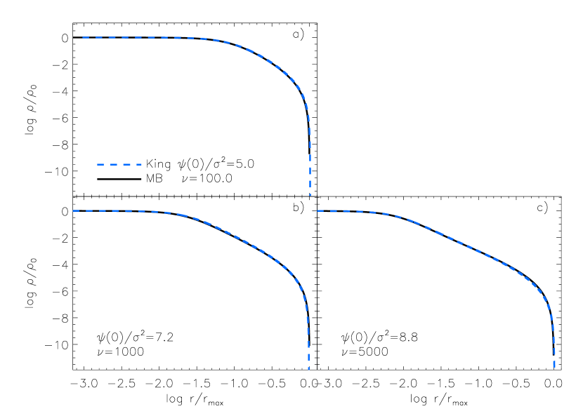
The MB case is intended to represent collisional systems because the co-habitation of the phase-space elements is allowed. The density profiles with $\nu=100$ and $1000$ are given in Figure 9a. The $r_{\rm max}$ scaling distance corresponds to the radius where a non-moving particle has an energy for which the distribution function disappears. The second panel of that figure (9b) shows the slope of the logarithmic density profile $\alpha$ along with curves corresponding to three other well-known analytical density profiles. These MB solutions are basically identical to King models (see Figure 10). This result comes as no surprise in the light of Madsen (1996), who did not use any approximation for $\ln x!$, and obtained density profiles very similar to King’s. In effect, abandoning the Stirling approximation and treating the low occupation number limit with the respect it apparently deserves, demonstrates that the King distribution function is the result of maximizing entropy in MB statistics, under the conditions of fixed mass and energy.

The consequence of using a very good smooth approximation to $\ln x!$, as done here, instead of the exact expression which gives discrete step-like values, as was done in Madsen (1996), is that the former results in spot-on matches to the King profiles, while the latter display modest differences from the King profile shape, especially for low $\Psi(0)/\sigma$ values; see Figure 1 Madsen (1996).

The value of $\nu$ appears to play a role analogous to the King scaling factor $\Psi(0)/\sigma^{2}$, where $\Psi(0)$ is a relative potential energy at the center, and $\sigma$ is an energy scaling constant (Binney & Tremaine, 1987). Increasing $\nu$—or $\Psi(0)/\sigma^{2}$—increases the concentration of the system. Recall that the higher the concentration, the closer the King model is to an isothermal sphere.

We find that the concentrations of the King models that most closely resemble the Maxwell-Boltzmann density profiles increase as the value of $\nu$ increases. Recall that $\nu$ is the number of fine-grained micro-cells that occupy a coarse-grained macro-cell, so as $\nu$ increases the distribution function becomes “grainier”. At the same time, increasing the concentration of a King model makes it more closely resemble an isothermal sphere. Putting these two observations together implies that increasing the coarseness of the distribution function (by increasing the number of fine-grained cells contained in a coarse-grained cell) should result in densities that have more isothermal aspects.

Finally, we note that both of the families of profiles obtained here have flat density cores, while cosmologically simulated halos have density cusps.

4.2. Results of Entropy Production Extremization

Some aspect of simulations may delay, or even disallow, the maximizing of entropy necessary to achieve thermal equilibrium. In such a frustrated case, it is possible that a collisionless system finds a stationary state by extremizing its entropy production. As a more concrete example of this situation, imagine a metal bar with one end exposed to a blowtorch and the other end in an ice bath. When the bar reaches a stationary state with a time-independent, but spatially varying, temperature distribution, entropy production in the bar is an extremum (de Groot & Mazur, 1984, Ch. 5, Sec. 3). We have begun to explore the possibility that the mechanical equilibria of simulated collisionless systems can be explained as states of extreme entropy production.

To this end, we have derived expressions for entropy production in collisionless systems using the Lynden-Bell statistics, and in collisional systems, using Maxwell-Boltzmann statistics. Further, we have found the form of the relaxation function required to guarantee an entropy production extreme. Recall that the relaxation function is the right-hand side of the Boltzmann equation, Equation 6, that describes the coarse-grained distribution function evolution.

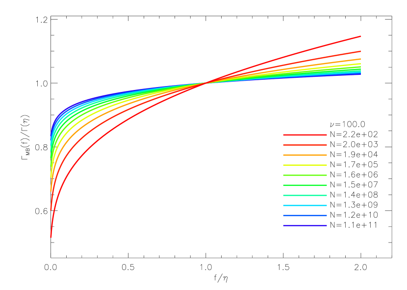
As in our previous work which was valid only for large phase-space occupation numbers, the Maxwell-Boltzmann relaxation function (pictured in Figure 6) is positive for all values of $F$ (as long as $N>1$) and becomes more constant as the number of particles $N$ increases. It is clear that the basic form of the relaxation function is not dependent on the specifics of the distribution function. A visual comparison between Figure 6 and Figure 1 in Barnes & Williams (2011) reinforces this point.

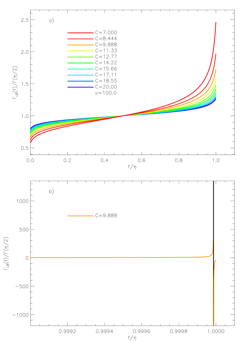
The general form of the Lynden-Bell relaxation function shown in Figure 7 has similarities and differences with its large occupation number version derived in Barnes & Williams (2011). The similarities are that both the functions increase with $f/\eta$ up to just short of $f/\eta=1$, then spike towards large positive values of $\Gamma_{LB}$, go through a singularity at $f/\eta\hbox{\hbox to0.0pt{\raise 1.82986pt\hbox{$<$}\hss}\lower 2.79857pt\hbox{$\sim$}}1$, then become negative, and eventually asymptote to $\Gamma_{LB}=0$ as $f/\eta\rightarrow 1$ (see the bottom panel of Figure 7). The difference is that the large occupation number $\Gamma_{LB}$ is independent of $\nu$, while its arbitrary occupation number analogue is not. In the latter case the values of $C$ and $\nu$ that produce the singularity are linked through the relationship,

$$\log{\frac{\nu_{\rm min}}{100}}=0.4348(C-4.1518),$$ (29)

where $\nu_{\rm min}$ is the minimum value of $\nu$ that will cause a singularity for a given $C$. This expression is valid as long as $\nu_{\rm min}\gtrsim 10$. The importance of the singularity in both cases is that it signals that the relaxation function will reach zero when the coarse-grained distribution function $f$ reaches the fine-grained value $\eta$, bringing the evolution of the distribution function to a halt.

To sum up, extremizing entropy production in the LB case leads to a relaxation function $\Gamma_{LB}$ vs. $f/\eta$ shape that drives $\Gamma_{LB}$, and hence the entropy production rate $\sigma_{Lb}$, to zero, which in turn means that the endpoint of evolution has a maximum (more correctly, an extremum) entropy. In other words, the entropy production extremization procedure that we followed in Section 3.2 tell us that the final state of a self-gravitating collisionless system is a state of maximum entropy. Since in Section 3.1 we derived such a state, using entropy maximization, it must be the same state.

The important point in both the LB and the MB case is that extremizing entropy production leads to relaxation functions that drive a coarse-grained distribution function to behave like a fine-grained distribution function. This has a bearing on the ‘incompleteness of relaxation’, sometimes alluded to when describing stationary-state collisionless systems. Our results suggest that if incomplete relaxation does happen, it is not due to a system reaching an entropy production extreme. Rather, it appears that coarse-grained evolution will proceed until entropy production ceases, when $\Gamma=0$, and so full relaxation will be achieved in self-gravitating systems. As an immediate consequence we conclude that entropy maximization is the correct—and more direct—procedure to take to arrive at the description of steady-state self-gravitating systems.

To test the hypothesis that for self-gravitating systems the state of entropy production extreme coincides with the state of maximum entropy, we are undertaking a comparison between these analytical descriptions of entropy behavior in collisionless systems and results of $N$-body and semi-analytical simulations (e.g., the extended secondary infall model ESIM Williams, Babul, & Dalcanton, 2004; Austin et al., 2005). This further work will help settle exactly what role entropy production plays in determining collisionless equilibria.

4.3. Outstanding Questions

Aside from the future work described above, to quantify entropy production rate in simulated numerical systems, there are also a few questions that remain unanswered.

4.3.1 Maximizing Entropy in Phase-space vs. Energy-space

Hjorth & Williams (2010) and the present paper maximized entropy, but in different state-spaces, energy and $(\boldsymbol{x},\boldsymbol{v})$ phase-space, respectively. The results of the two studies, for example in terms of the density profiles, are very different from each other. It is not surprising that they are different, but it is not immediately obvious which one of the two approaches would produce a better description of the results of collisionless N-body simulations. After looking at all the density profiles it is seen that Hjorth & Williams (2010) profiles are similar to those of simulated systems (Williams & Hjorth, 2010; Williams et al., 2010), while those from the LB case in the present work (Section 3.1, Figures 4 and 5) are not.

We note that our LB entropy maximization results are what Lynden-Bell (1967) would have obtained had he not used the Stirling approximation. The procedure does not rely on any approximations, and is well motivated from first principles, assuming that all states are equally accessible and efficient mixing in phase-space can be achieved. This begs the question, do such systems exist? More work with simulations is needed to address this question.

4.3.2 The Necessity of the Low Occupation Number Regime

Our MB entropy maximization results of Section A.1 (and the very similar results of Madsen, 1996) describe some globular clusters well (Elson et al., 1987; Meylan & Heggie, 1997; Williams et al., 2011), and the results of Hjorth & Williams (2010) describe N-body and ESIM halos. These facts lead us to the following chain of reason. First, globular clusters, along with N-body and ESIM halos, are self-gravitating systems. Second, the entropy maximization procedures that produce successful models of these systems require correct treatment of low phase-space occupation numbers. Therefore, it appears that the low occupation number regime is an important distinction between self-gravitating and non-self-gravitating systems.

Why is this the case? We speculate that self-gravitating systems are special not only because they are finite in extent due to the long-range nature of the force, but also because of correlations between spatial regions and energies of particles. Specifically, the center of the potential contains phase-space elements with the most bound energies, while the outskirts are populated by elements with the least bound, or even zero energies. These requirements are peculiar to self-gravitating systems, and apparently necessitate low occupation numbers because the numbers of particles in these regions must approach zero.

However, the above hypothesis does not explain why the discrete version of $\ln x!$ must be smoothed to represent real systems. This smoothing, though apparently necessary, is still not well justified.

4.3.3 Should Maximum Entropy Imply Constant Temperature?

The steady-state of self-gravitating systems can apparently be calculated as the maximum entropy state. Though these systems are in mechanical equilibrium, one could argue that they are not in conventional thermal equilibrium because their kinetic temperature is manifestly different across the system. Can we reconcile maximum entropy defining thermodynamic equilibrium with the resulting non-constant temperature? (Note that a realistic self-gravitating system cannot have a constant kinetic temperature, because there is no finite-mass solution to the Jeans equation with constant $\sigma$.) This contradiction is part of the reason why it made sense to conclude, based on Lynden-Bell (1967) work that there is no maximum entropy state for self-gravitating systems.

We propose that for gravitationally-bound collisionless systems, one must carefully separate kinetic temperature $T_{k}$ from thermodynamic temperature $T_{t}$. To be clear, the kinetic temperature we are referring to is related to the rms value of the peculiar velocity in a system, $T_{k}\propto\langle v_{p}^{2}\rangle$. The thermodynamic temperature is linked to the energy scale $\beta$ that serves as a Lagrange multiplier through $\beta=1/(k_{B}T_{t})$. By definition, $T_{t}$ must be a constant, and there is no contradiction as in Lynden-Bell (1967)—systems in the maximum entropy state are characterized by a constant thermodynamic temperature, even as they have a varying kinetic temperature.

We can also address a related question involving the temperature and energy change that appear in the thermodynamic definition of entropy, $\mathrm{d}S=\delta Q/T$. This temperature must be a constant, so we would associate this with the thermodynamic temperature $T_{t}$. $\delta Q$ (normally called heat) refers to all non-work exchanges of energy, and so must be replaced by $\delta\epsilon$ because in collisionless self-gravitating systems what is being transferred is total energy, potential and kinetic, not just kinetic. Entropy changes can occur due to changes in mass distribution as well as kinetic energy transport.

Appendix A Maxwell-Boltzmann Statistics

A.1. Entropy Maximization

Using the results of § 1.3, the multiplicity function for a system obeying MB statistics combined with the definition of entropy (Equation 1) produces,

$$S_{\rm MB}=k_{\rm B}\left[\ln{N!}-\sum_{i}\ln{n_{i}!}+N\ln{\nu}\right],$$ (A1)

where the summation involving the macro-cell occupation $n_{i}$ runs over the number of macro-cells. We will assume that $N\gg 1$, so that $\ln{N!}=N\ln{N}-N$. However, we will not use the Stirling approximation for the second term on the right-hand side of Equation A1. With our approximation, Equation 12, we can now rewrite the entropy as,

$$S_{\rm MB}=S_{\rm MB,0}-k_{\rm B}\sum_{i}\left[(n_{i}+1/2)\ln{(n_{i}+1)}+\lambda_{0,n_{i}}\right],$$ (A2)

where $S_{\rm MB,0}=Nk_{\rm B}[\ln{(N\nu)}-M\ln{2\pi}/2N]$ is a constant, and $M$ is the total number of macro-cells.

We now replace the discrete macro-cell occupation number $n_{i}$ with the coarse-grained distribution function $f$ to produce

$$S_{\rm MB}=S_{\rm MB,0}-\frac{k_{\rm B}}{\nu\varpi}\iint\left[\left(\frac{\nu f}{\eta}+1/2\right)\ln{\left(\frac{\nu f}{\eta}+1\right)}+\lambda_{0,\nu f/\eta}\right]\>\mathrm{d}\boldsymbol{x}\>\mathrm{d}\boldsymbol{v}.$$ (A3)

To maximize this entropy function, we set $\delta S_{\rm MB}=0$, subject to constant mass and energy constraints. The expression that results is,

$$\ln{\left(\frac{\nu f}{\eta}+1\right)}+\frac{(\nu f/\eta+1/2)}{(\nu f/\eta+1)}+\frac{\eta}{\nu}\frac{\partial\lambda_{0,\nu f/\eta}}{\partial f}+\mu+\beta\epsilon=0,$$ (A4)

where $\mu$ and $\beta$ are undetermined multipliers associated with mass and energy conservation, respectively. The $\epsilon$ term is the specific energy of a phase element located at position $\boldsymbol{x}$ with velocity $\boldsymbol{v}$, $\epsilon=v^{2}/2+\Phi$. Note that if the standard Stirling approximation had been employed, the second and third terms would be absent and the logarithmic term would simply read $\ln{(\nu f/\eta)}$. In this case, the usual, physically inconsistent, MB distribution function would result.

As before, we make a change of variables, $F\equiv\nu f/\eta$, and the derivative of the $\lambda$ function is given by Equations 16. Equation A4 can then be re-cast as,

$$\ln{(F+1)}-\frac{(264F+276)}{576(F+1)(F+600/576)}+\mu+\beta\epsilon=0.$$ (A5)

Again, we have not searched for an analytical solution, but graphical solutions for $F$ for a range of $\epsilon$ values can be combined to produce a plot of $F(\epsilon)$. Specifically, Figure 8 illustrates the behavior of the normalized coarse-grained distribution function $f/\eta$ for a particular value of $\nu$. Values of the Lagrange multipliers $\mu$ and $\beta$ were adjusted so that $\epsilon$ is always positive. Because MB statistics have no exclusion principle, $f/\eta$ can have values above 1.

A.2. Entropy Production Extremization

We begin by writing entropy in terms of entropy density,

$$S=\int\rho s\>\mathrm{d}\boldsymbol{x},$$ (A6)

where $\rho$ is mass density, $s$ is the specific entropy, and the integral is taken over the spatial extent of the system. From the entropy form given in Equation A3, the entropy density can now be written as,

$$\rho s_{\rm MB}=-\frac{k_{\rm B}}{\nu\varpi}\int\left[(F+1/2)\ln{(F+1)}+\lambda_{0,F}-F\frac{S_{\rm MB,0}}{Nk_{\rm B}}\right]\>\mathrm{d}\boldsymbol{v},$$ (A7)

where, as earlier, $F=\nu f/\eta$.

Taking a partial time derivative of Equation A7 results in,

$$\frac{\partial}{\partial t}(\rho s_{\rm MB})=-\frac{k_{\rm B}}{\nu\varpi}\int\frac{\partial F}{\partial t}\left[\ln{\left(F+1\right)}+\frac{(F+1/2)}{(F+1)}+\frac{\partial\lambda_{0,F}}{\partial F}-B\right]\>\mathrm{d}\boldsymbol{v},$$ (A8)

where $B=S_{\rm MB,0}/Nk_{\rm B}$ is a constant.

Substituting $\partial F/\partial t$ from the Boltzmann equation into Equation A8 results in a lengthy expression, similar to Equation 22 in the Lynden-Bell case. We will deal with this expression term by term. For reference, the expression after substitution is,

$$\frac{\partial}{\partial t}(\rho s_{\rm MB}) = -\frac{k_{\rm B}}{\nu\varpi}\int(-\boldsymbol{v}\boldsymbol{\cdot}\boldsymbol{\nabla}F)\left[\ln{(F+1)}+\frac{(F+1/2)}{(F+1)}+\frac{\partial\lambda_{0,F}}{\partial F}-B\right]\>\mathrm{d}\boldsymbol{v}-$$ (A9)

$$\frac{k_{\rm B}}{\nu\varpi}\int(-\boldsymbol{a}\boldsymbol{\cdot}\boldsymbol{\nabla}_{v}F)\left[\ln{(F+1)}+\frac{(F+1/2)}{(F+1)}+\frac{\partial\lambda_{0,F}}{\partial F}-B\right]\>\mathrm{d}\boldsymbol{v}+$$

$$\frac{k_{\rm B}}{\nu\varpi}\int\gamma\left[\ln{(F+1)}+\frac{(F+1/2)}{(F+1)}+\frac{\partial\lambda_{0,F}}{\partial F}-B\right]\>\mathrm{d}\boldsymbol{v},$$

where $\gamma=(\nu\Gamma)/\eta$.

The process to evaluate these integrals is very similar to what has been discussed in the Lynden-Bell case. Using the fact that $\boldsymbol{v}\boldsymbol{\cdot}\boldsymbol{\nabla}F=\boldsymbol{\nabla}\boldsymbol{\cdot}F\boldsymbol{v}$, the first integral on the right-hand side of Equation A9 can be re-written as,

$$-\boldsymbol{\nabla}\boldsymbol{\cdot}\int\left[(F+1/2)\ln{(F+1)}+\lambda_{0,F}-FB\right]\boldsymbol{v}\>\mathrm{d}\boldsymbol{v}.$$ (A10)

Note that this expression is reminiscent of the form of the entropy density in Equation A7.

We next turn our attention to the terms involving acceleration in Equation A9. The fact that $\boldsymbol{a}$ is velocity-independent implies that $\boldsymbol{a}\boldsymbol{\cdot}\boldsymbol{\nabla}_{v}f=\boldsymbol{\nabla}_{v}\boldsymbol{\cdot}\boldsymbol{a}f$, a fact that will be used often in dealing with these terms. Let us start with the first part of the the second term on the right-hand side of Equation A9,

$$\int(-\boldsymbol{a}\boldsymbol{\cdot}\boldsymbol{\nabla}_{v}F)\ln{(F+1)}\>\mathrm{d}\boldsymbol{v}=-\int(\boldsymbol{\nabla}_{v}\boldsymbol{\cdot}\boldsymbol{a}F)\ln{(F+1)}\>\mathrm{d}\boldsymbol{v}.$$ (A11)

Integrating by parts produces two terms, one with the form,

$$\boldsymbol{\nabla}_{v}\boldsymbol{\cdot}[\boldsymbol{a}F\ln{(F+1)}]\>\mathrm{d}\boldsymbol{v}.$$ (A12)

which equals zero after using the divergence theorem and the fact that any physical distribution function must vanish for large velocities. The other term resulting from the integration by parts is,

$$\boldsymbol{a}\boldsymbol{\cdot}\int\left(\boldsymbol{\nabla}_{v}F\right)\frac{F}{F+1}\>\mathrm{d}\boldsymbol{v}=\boldsymbol{a}\boldsymbol{\cdot}\int\boldsymbol{\nabla}_{v}\left[(F+1)-\ln{(F+1)}\right]\>\mathrm{d}\boldsymbol{v}.$$ (A13)

A single component of this integral will appear as,

$$\int_{v_{1,min}}^{v_{1,max}}\frac{\partial}{\partial v_{1}}\left[(F+1)-\ln{(F+1)}\right]\>\mathrm{d}v_{1}=(F+1)-\ln{(F+1)}|_{v_{1,min}}^{v_{1,max}},$$ (A14)

where $v_{1,min}=-v_{1,max}$, representing the maximum speed possible for the system. Assuming that $F$ is even in $v_{1,max}$ and that $F(v_{1,max})=0$ so that the distribution function disappears at the maximum speed, this integration results in zero. Similar manipulations can be applied to the rest of the acceleration-dependent parts of the second term on the right-hand side of Equation A9, resulting in the entire second term being equal to zero. Equation A9 now has the form,

$$\frac{\partial}{\partial t}(\rho s_{\rm MB}) = -\frac{k_{\rm B}}{\nu\varpi}\left\{-\boldsymbol{\nabla}\boldsymbol{\cdot}\int\left[(F+1/2)\ln{(F+1)}+\lambda_{0,F}-FB\right]\boldsymbol{v}\>\mathrm{d}\boldsymbol{v}+\right.$$ (A15)

$$\left.\int\gamma(F)\left[\ln{(F+1)}+\frac{F+1/2}{F+1}+\frac{\partial\lambda_{0,F}}{\partial F}-B\right]\right\}\>\mathrm{d}\boldsymbol{v}.$$

Assuming the velocity field to be composed of mean and peculiar components $\boldsymbol{v}=\boldsymbol{v_{0}}+\boldsymbol{v_{p}}$, we can re-cast Equation A15 as,

$$\frac{\partial}{\partial t}(\rho s_{\rm MB}) = -\boldsymbol{\nabla}\boldsymbol{\cdot}\rho s_{\rm MB}\boldsymbol{v_{0}}-\frac{k_{\rm B}}{\nu\varpi}\Bigg{\{}-\boldsymbol{\nabla}\boldsymbol{\cdot}\int\left[(F+1/2)\ln{(F+1)}+\lambda_{0,F}-FB\right]\boldsymbol{v_{p}}\>\mathrm{d}\boldsymbol{v}+$$ (A16)

$$\int\gamma(F)\left[\ln{(F+1)}+\frac{F+1/2}{F+1}+\frac{\partial\lambda_{0,F}}{\partial F}-B\right]\>\mathrm{d}\boldsymbol{v}\Bigg{\}}.$$

We now equate the terms in Equation A16 to those in the continuous version of the entropy density evolution equation, Equation 25,

$$\frac{\partial}{\partial t}(\rho s)=-\boldsymbol{\nabla}\boldsymbol{\cdot}(\boldsymbol{\Sigma}+\rho s\boldsymbol{v_{0}})+\sigma.$$ (A17)

The entropy flux $\boldsymbol{\Sigma}$ is given by the integral in the second term on the right-hand side of Equation A16 and represents randomly fluxed entropy. The remaining term is the entropy production for the system,

$$\sigma_{\rm MB}=-\frac{k_{\rm B}}{\nu\varpi}\int\gamma(F)\left[\ln{(F+1)}+\frac{F+1/2}{F+1}+\frac{\partial\lambda_{0,F}}{\partial F}-B\right]\>\mathrm{d}\boldsymbol{v}.$$ (A18)

This equation explicitly demonstrates how the non-collisionless nature of the coarse-grained distribution function leads to changes in entropy.

As mentioned in § 1, thermodynamic non-equilibrium systems can have steady-states described by extrema of entropy production. We then set $\delta\sigma_{\rm MB}=0$. Taking the variation of Equation A18, we find

$$\delta\sigma_{\rm MB}=-\frac{k_{\rm B}}{\nu\varpi}\int\delta F\left\{\frac{\mathrm{d}\gamma}{\mathrm{d}F}\left[\ln{(F+1)}+\frac{F+1/2}{F+1}+\frac{\mathrm{d}\lambda_{0,F}}{\mathrm{d}F}-B\right]+\gamma\left[\frac{2}{F+1}-\frac{F+1/2}{(F+1)^{2}}+\frac{\mathrm{d}^{2}\lambda_{0,F}}{\mathrm{d}F^{2}}\right]\right\}\>\mathrm{d}\boldsymbol{v}.$$ (A19)

Since $\delta F$ is arbitrary, the variation disappears only when the term in curly braces is zero. The condition for an extremum in entropy production is,

$$\frac{\mathrm{d}\ln{\gamma}}{\mathrm{d}F}\left[\ln{(F+1)}+\frac{F+1/2}{F+1}+\frac{\mathrm{d}\lambda_{0,F}}{\mathrm{d}F}-B\right]+\left[\frac{2}{F+1}-\frac{F+1/2}{(F+1)^{2}}+\frac{\mathrm{d}^{2}\lambda_{0,F}}{\mathrm{d}F^{2}}\right]=0.$$ (A20)

The solution for the Maxwell-Boltzmann relaxation function is,

$$\gamma_{\rm MB}(F)=P/\left[\ln{(F+1)}+\frac{F+1/2}{F+1}+\frac{\mathrm{d}\lambda_{0,F}}{\mathrm{d}F}-\frac{S_{\rm MB,0}}{Nk_{\rm B}}\right],$$ (A21)

where the constant can be expressed as

$$P=\gamma_{\rm MB}(F=\nu)\left[\ln{(\nu+1)}+\frac{\nu+1/2}{\nu+1}-\frac{\nu+1}{\nu+600/576}-(S_{\rm MB,0}/Nk_{\rm B})\right].$$ (A22)

The $\gamma_{\rm MB}(F=\nu)$ term is the relaxation function value when the coarse-grained distribution function is equal to the constant fine-grained distribution function value ($f=\eta$).

Figure 1.— A schematic summary of the various statistical mechanical approaches to self-gravitating systems. See Section 1.4 for explanation.

Figure 2.— Comparing the Stirling, Hjorth & Williams (2010) and Equation 9 approximations to $\ln{x!}$ as functions of $x$. The function $\psi(x+1)\equiv\mathrm{d}\ln{x!}/\mathrm{d}x$ is plotted. Note the divergent behavior of the Stirling approximation as $x\rightarrow 0$. (a) The raw $\psi$ functions for the three approximations are shown. The Hjorth & Williams (2010) line is very nearly covered by the Equation 9 line. (b) Differences between the various approximations and Equation 9. The differences between the Hjorth & Williams (2010) and Equation 9 approximations are much smaller than those between either approximation and the Stirling approximation. Also, the Hjorth & Williams (2010) and Equation 9 values coincide for $x=0$.

Figure 3.— The Lynden-Bell distribution function resulting from the non-Stirling approximation. The Lynden-Bell function derived using the Stirling approximation is also shown.

Figure 4.— (a) Logarithmic density and (b) the corresponding $\alpha=-\mathrm{d}\log{\rho}/\mathrm{d}\log{r}$ versus logarithmic scaled radius for the Lynden-Bell case. The thick solid black lines correspond to models with $\nu=100$ while the thick dashed black lines represent models with $\nu=1000$. The vertical lines mark where the logarithmic slope of the $\nu=100$ model is isothermal ($\alpha=2$). The $\alpha$ profiles for NFW, Navarro et al. (2004), and Plummer models are also shown. The profiles for the $\nu=1000$ model have been horizontally shifted so that the location where $\alpha=2$ coincides with the other models. The central cusp of the NFW and Navarro et al. (2004) models ($\alpha\rightarrow 1$ as $r\rightarrow 0$) differs markedly from the core present in the Lynden-Bell case ($\alpha\rightarrow 0$ as $r\rightarrow 0$). The presence of the core in the Lynden-Bell case is independent of $\nu$.

Figure 5.— Comparisons between Lynden-Bell (solid) and King (dashed) density profiles for different $\nu$ values; (a) $\nu=100$ and (b) $\nu=1000$. The King scale factors correspond to those used in Figure 10 for the same $\nu$ values. The shapes of the curves cannot be brought into agreement for any scale factor values.

Figure 6.— The behavior of the relaxation function $\Gamma_{\rm MB}$ as a function of the coarse-grained distribution function $f$ in a system that obeys Maxwell-Boltzmann statistics. The various lines represent functions defined with different $N$ values, where $N$ is the number of phase-space elements in a system. As with the LB case, as $N$ increases, the relaxation function becomes more constant. Note that the horizontal axis scale differs from that in Figure 7a since there is no restriction on the value of the coarse-grained distribution function in the MB case. All curves correspond to cases where $\nu=100$.

Figure 7.— The behavior of the relaxation function $\Gamma_{\rm LB}$ as a function of the coarse-grained distribution function $f$ in a system that obeys Lynden-Bell statistics. Panel a includes various lines representing functions defined with different $C$ values, where $C=\ln{N}-1+M/N(\nu\ln{\nu}-\ln{2\pi})$. $N$ is the number of phase-space elements in a system, and increasing $N$ results in increasing $C$. As $N$ increases, the relaxation function becomes more constant. All curves correspond to cases where $\nu=100$. As $\nu$ increases, these curves develop singularities near $f=\eta$, as shown in panel b.

Figure 8.— The natural logarithm of the Maxwell-Boltzmann distribution function resulting from the non-Stirling approximation. The Maxwell-Boltzmann function derived using the Stirling approximation is also shown. The non-Stirling approximation distribution function reaches zero for a finite $\epsilon$, unlike the exponential function derived using the Stirling approximation.

Figure 9.— (a) Logarithmic density and (b) the corresponding $\alpha=-\mathrm{d}\log{\rho}/\mathrm{d}\log{r}$ versus logarithmic scaled radius for the Maxwell-Boltzmann case. The thick solid black lines represent models with $\nu=100$ while the thick dashed black lines correspond to models with $\nu=1000$. The vertical lines mark where the logarithmic slope of the $\nu=100$ model is isothermal ($\alpha=2$). The $\alpha$ profiles for NFW, Navarro et al. (2004), and Plummer models are also shown. As in Figure 4, the $\nu=1000$ curve has been shifted horizontally to align the locations where $\alpha=2$. The central cusp of the NFW and Navarro et al. (2004) models ($\alpha\rightarrow 1$ as $r\rightarrow 0$) differs markedly from the core present in the Maxwell-Boltzmann case ($\alpha\rightarrow 0$ as $r\rightarrow 0$). The presence of the core in the Maxwell-Boltzmann case is independent of $\nu$.

Figure 10.— Comparisons between Maxwell-Boltzmann (solid) and King (dashed) density profiles for different $\nu$ values; (a) $\nu=100$, (b) $\nu=1000$, (c) $\nu=5000$. The King profile scale factor $\Psi(0)/\sigma^{2}$ is given in each panel. The dashed lines represent King density profiles while the solid lines show the Maxwell-Boltzmann distributions. The comparison between these two profile types reveals more similarity than when the Madsen (1996) and King models are compared.

References

- Aly (1994) Aly, J.-J. 1994, in Lecture Notes in Physics, Vol. 430, Ergodic Concepts in Stellar Dynamics, ed. V. G. Gurzadyan and D. Pfenniger, (New York, NY: Springer-Verlag), 226
- Austin et al. (2005) Austin, C. G., Williams, L. L. R., Barnes, E. I., Babul, A., Dalcanton, J. J. 2005, ApJ, 634, 756
- Barnes & Williams (2011) Barnes, E. I., Williams, L. L. R. 2011, ApJ, 728, 136 (BWI)
- Binney & Tremaine (1987) Binney, J., Tremaine, S. 1987, Galactic Dynamics, (Princeton, NJ:Princeton)
- Chavanis (1998) Chavanis, P. H. 1998, MNRAS, 300, 981
- de Groot & Mazur (1984) de Groot, S. R., Mazur, P. 1984, Non-Equilibrium Thermodynamics, (Mineola, NY:Dover)
- Elson et al. (1987) Elson, R., Hut, P., Inagaki, S. 1987, ARA&A, 25, 565
- Grandy (2008) Grandy, W. T. 2008, Entropy and the Time Evolution of Macroscopic Systems, (New York, NY:Oxford)
- Hjorth & Williams (2010) Hjorth, J., Williams, L. L. R. 2010, ApJ, 722, 851 (HW10)
- Huss et al. (1999) Huss, A., Jain, B., Steinmetz, M. 1999, ApJ, 517, 64
- Jaynes (1980) Jaynes, E. T. 1980, Annual Review of Physical Chemistry, ed. S. Rabinovich, (Palo Alto, CA: Annual Reviews)
- King (1966) King, I.R. 1966, AJ, 71, 64 (K66)
- Lynden-Bell (1967) Lynden-Bell, D. 1967, MNRAS, 136, 101 (LB67)
- Madsen (1996) Madsen, J. 1996, MNRAS, 280, 1089 (M96)
- Meylan & Heggie (1997) Meylan, G., Heggie, D.C. 1997, ARA&A, 8,1
- Navarro et al. (1996) Navarro, J. F., Frenk, C. S., White, S. D. M. 1996, ApJ, 462, 563
- Navarro et al. (2004) Navarro, J. F., Hayashi, E., Power, C., Jenkins, A. R., Frenk, C. S., White, S. D. M., Springel, V., Stadel, J., Quinn, T. R. 2004, MNRAS, 349, 1039
- Ogorodnikov (1957) Ogorodnikov, K.F. 1957, Soviet Astronomy, 1, 748
- Plummer (1911) Plummer, H. C. 1911, MNRAS, 71, 460
- Prigogine (1961) Prigogine, I. 1961, Thermodynamics of Irreversible Processes, (New York, NY: Interscience)
- Schuster (1883) Schuster, A. 1883, British Assoc. Report, 427
- Simons (1994) Simons, S. 1994, Am. J. of Phys., 62, 515
- Stiavelli & Bertin (1987) Stiavelli, M., Bertin, G. 1987, MNRAS, 229, 61
- Tremaine, Hénon, & Lynden-Bell (1986) Tremaine, S., Hénon, M., Lynden-Bell, D. 1986, MNRAS, 219, 285
- van Albada (1982) van Albada, T. S. 1982, MNRAS, 201, 939
- White & Narayan (1987) White, S. D. M., Narayan, R. 1987, MNRAS, 229, 103
- Williams, Babul, & Dalcanton (2004) Williams, L. L. R., Babul, A., Dalcanton, J. J. 2004, ApJ, 604, 18
- Williams & Hjorth (2010) Williams, L.L.R. & Hjorth, J. 2010, ApJ, 722, 856
- Williams et al. (2010) Williams, L.L.R., Hjorth, J. & Wojtak, R. 2010, ApJ, 725, 282
- Williams et al. (2011) Williams, L.L.R., Barnes, E.I. & Hjorth, J. 2011, MNRAS, submitted