A new stochastic differential equation modelling incidence and prevalence with an application to systemic lupus erythematosus in England and Wales, 1995

Abstract

This article reformulates a common illness-death model in terms of a new system of stochastical differential equations (SDEs). The SDEs are used to estimate epidemiological characteristics and burden of systemic lupus erythematosus in England and Wales in 1995.

Keywords: Chronic diseases; Incidence; Prevalence; Mortality; Systemic lupus erythematosus; Stochastic differential equation.

1 Introduction

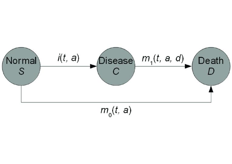
With a view to basic epidemiological parameters such as incidence, prevalence and mortality of a disease, it has proven useful to consider so called state models or compartmental models. The model used here is also termed illness-death model (Kalbfleisch and Prentice, 2002, Fig. 8.4). It consists of the three states Normal, Disease, Death and the transitions between the states. Normal means non-diseased with respect to the disease under consideration. The numbers of persons in the Normal and Disease state are denoted as $S$ (susceptibles) and $C$ (cases), respectively. The transition intensities (synonymously: rates) are called as shown in Figure 1: $i$ is the incidence rate, $m_{0}$ and $m_{1}$ are the mortality rates of the non-diseased and diseased persons, respectively. In general, the intensities depend on calendar time $t$, age $a$ and sometimes also on the duration $d$ of the disease.

Figure 1: Illness-death model of a chronic disease with three states. Persons in the state Normal are healthy with respect to the considered disease. In the state Disease they suffer from the disease. In the most general case, the transition rates depend on the calendar time $t,$ age $a,$ and in case of the disease-specific mortality $m_{1}$ also on the disease’s duration $d$.

When the rates do not depend on calendar time $t$, the model is called time-homogeneous. Then, with the additional condition that there is no dependency on the duration, Murray and Lopez have considered a two-dimensional system of ordinary differential equations (ODEs) to relate the changes of the numbers of healthy and diseased persons with the rates of the in- and outflows of the corresponding states (1994):

$$\begin{split}\frac{\mathrm{d}S}{\mathrm{d}a}&=-\bigl{(}i(a)+m_{0}(a)\bigr{)}\cdot S\\ \frac{\mathrm{d}C}{\mathrm{d}a}&=i(a)\cdot S-m_{1}(a)\cdot C.\\ \end{split}$$ (1)

Age $a$ plays the role of temporal progression. The linear system (1) looks relatively harmless, but the impression is misleading. Mostly only the age-specific mortality of the general population is well known, and rate $m_{1}$ is epidemiologically accessible as relative risk. Then, the system becomes nonlinear.

Furthermore, the inclusion of the hypothetical values $S$ and $C$ is disturbing. It would be better if we had the age-specific prevalence $p(a):=\tfrac{C(a)}{S(a)+C(a)}$ here, what indeed can be achieved (Brinks, 2011).

What are the benefits of such ODEs? For smooth incidence- and mortality rates plus an initial condition, the age profile of the numbers of patients or the prevalence is uniquely determined. To state it clearly, the “forces” incidence and mortality uniquely prescribe the prevalence – not only qualitatively but in these quantitative terms. In this, we speak of the forward problem: we close from the causes – the forces – to the effect, namely the number of diseased persons. The reverse way, closing from the numbers of diseased persons to the incidence, is the inverse problem – we infer from the effect to the cause.

This paper is structured as follows: in the next section we describe the illness-death model of Figure 1 in terms a new system of two stochastic differential equations (SDEs). As an application, in Section 3 we solve a forward problem to estimate the age-specific prevalence of systemic lupus erythematosus (SLE) in England and Wales from published data. This allows calculation of the mean age at onset of SLE, the mean duration and the burden of SLE in terms of diseased persons.

2 Stochastic description of the illness-death model

What can be achieved in the domain of ODEs, dividing the number $C(a)$ of the diseased by the number $S(a)+C(a)$ of the living for deriving the prevalence at age $a$, is not that easy in random variables. Distributions of quotients of stochastically dependent random variables are problematic, so we have to model $S$ and $C$ bivariately.

Let $X(a):=\left(S(a),C(a)\right)^{t}$ be the composite vector (the superscript denotes transposition). For $\Delta a>0$ define the vector $\Delta X$ of increments:

$$\Delta X(a):=\bigl{(}S(a+\Delta a)-S(a),C(a+\Delta a)-C(a)\bigr{)}^{t}$$

Now we follow the reasoning of (Allen, 1999) and (Allen, 2008), who have applied the theory presented here in the field of infectious diseases modeling.

Choose $\Delta a>0$ small that at most one person can change the state. In accordance with the definition of the rates $i$, $m_{0}$ and $m_{1}$ the following assumptions about the probability distribution $P(\Delta X(a))$ are made:

$$P\left(\Delta X(a)={u\choose v}\right)=\begin{cases}m_{0}(a)\cdot S(a)\cdot\Delta a+o(\Delta a)&\textnormal{if }(u,v)=(-1,0)\\ m_{1}(a)\cdot C(a)\cdot\Delta a+o(\Delta a)&\textnormal{if }(u,v)=(0,-1)\\ i(a)\cdot S(a)\cdot\Delta a+o(\Delta a)&\textnormal{if }(u,v)=(-1,1)\\ 1-\bigl{[}m_{0}(a)\cdot S(a)+m_{1}(a)\cdot C(a)+&\\ ~{}~{}~{}~{}~{}~{}~{}i(a)\cdot S(a)\bigr{]}\cdot\Delta a+o(\Delta a)&\textnormal{if }(u,v)=(0,0)\\ \end{cases}$$ (2)

If we further assume that the increments are normally distributed, we get the expected value

$$E\bigl{(}\Delta X(a)\bigr{)}=\left[m_{0}(a)\cdot S(a)\cdot{-1\choose 0}+m_{1}(a)\cdot C(a)\cdot{0\choose-1}+i(a)\cdot S(a)\cdot{-1\choose 1}\right]\cdot\Delta a+o(\Delta a)$$

and covariance matrix

$$\begin{split}V\bigl{(}\Delta X(a)\bigr{)}&=E\left(\Delta X(a)\cdot\Delta X^{t}(a)\right)-E\left(\Delta X(a)\right)\cdot E\left(\Delta X^{t}(a)\right)\\ &\approx E\left(\Delta X(a)\cdot\Delta X^{t}(a)\right).\end{split}$$

The matrix $V$ is symmetric and positively definite. Hence, there is uniquely determined matrix square root $V^{1/2}$. Due the normal distribution assumption the vector $X$ fulfills

$$X(a+\Delta a)=X(a)+\Delta X(a)=X(a)+E\bigl{(}\Delta X(a)\bigr{)}+V\bigl{(}\Delta X(a)\bigr{)}^{1/2}\,\xi,$$ (3)

where $\xi=(\xi_{1},\xi_{2})^{t}$ has normally distributed components $\xi_{i}\sim N(0,1),~{}i=1,2.$

Under certain smoothness conditions about the coefficient functions $i,m_{1}$ and $m_{0}$ the difference equation (3) is an Euler approximation to the Îto SDE system

$$\begin{split}\frac{\mathrm{d}S}{\mathrm{d}a}&=-\bigl{(}i(a)+m_{0}(a)\bigl{)}\cdot S+b_{11}\frac{\mathrm{d}W_{1}}{\mathrm{d}a}+b_{12}\frac{\mathrm{d}W_{2}}{\mathrm{d}a}\\ \frac{\mathrm{d}C}{\mathrm{d}a}&=i(a)\cdot S-m_{1}(a)\cdot C+b_{21}\frac{\mathrm{d}W_{1}}{\mathrm{d}a}+b_{22}\frac{\mathrm{d}W_{2}}{\mathrm{d}a}.\\ \end{split}$$ (4)

In this expression, $W_{1}$ and $W_{2}$ are independent Wiener processes (Kloeden and Platen, 1999) and the $2\times 2$ – matrix $B=(b_{ij})$ is the uniquely determined square root of the covariance matrix divided by $\Delta a$:

$$B=\bigl{(}V(\Delta X)/\Delta a\bigr{)}^{1/2}.$$

Which advantages has the SDE formulation compared to the ODE? In rare diseases as in the next section, the inclusion of uncertainty is sometimes more appropriate than calculating deterministically. In addition, SDEs sometimes have properties that cannot be derived from the theory of ODEs, as for example the quasistationary solutions (Darroch and Seneta, 1967).

3 Application to Systemic Lupus Erythematosus

In this section the SDE is applied to epidemiological data of systemic lupus erythematosus in England and Wales. Systemic lupus erythematosus (SLE) is a severe rheumatic disease with a variety of clinical manifestations. Despite several therapy options, patients often are restricted heavily in quality of life and ability to work. Epidemiological data are rare. Here, the incidence data for males and females is taken from the UK General Practice Research Database (GPRD) in the years 1990–1999 as reported in (Somers et al., 2007). Mortality $m_{1}$ of SLE patients is modeled by the relative mortality as reported in (Bernatsky et al., 2006). Duration of SLE was not taken into account.

Regarding the mortality of the non-diseased, we take the mortality in the general population. Due to the low prevalence of SLE this is legitimate. Then, 5000 solution paths of the SDE system (4) are simulated by the Euler-Maruyama method (Kloeden and Platen, 1999) and the corresponding age-specific prevalences have been calculated. This is done for males and females separately.

As an example, Figure 2 shows the prevalence resulting from two pairs of solution paths.

Figure 2: Example paths of the age-specific prevalence of SLE resulting from two pairs of solution paths of system (4).

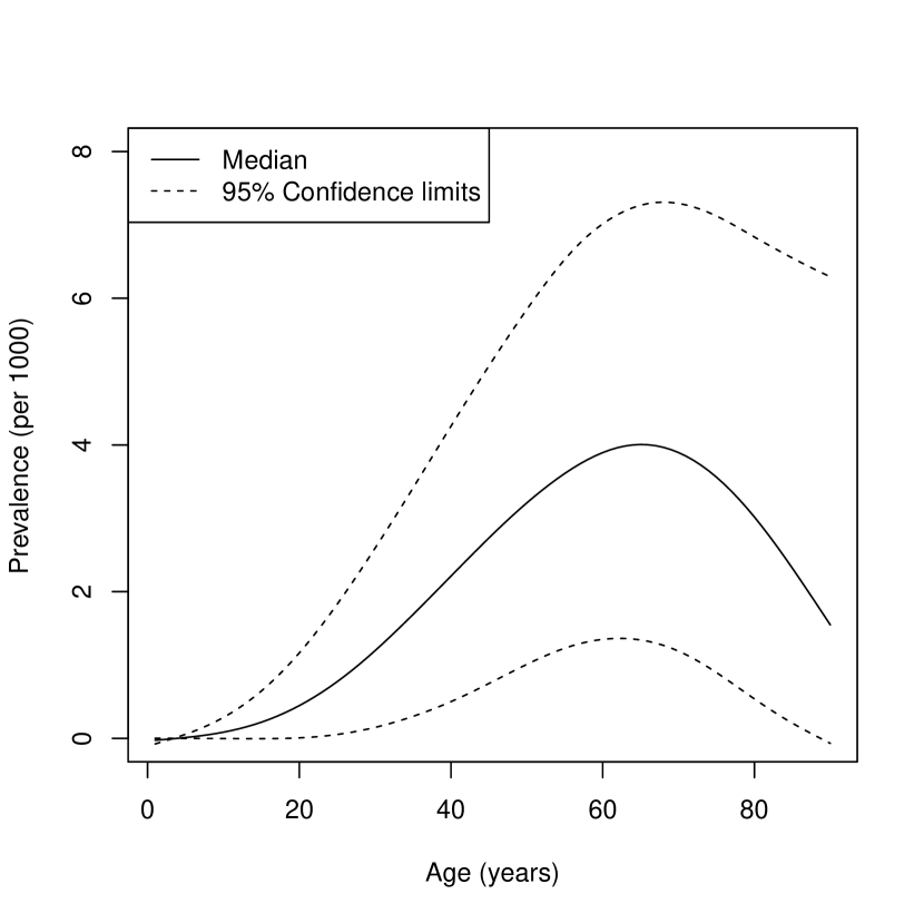
Of course, single paths for the prevalence are not that important. It is more interesting, to analyze where the paths of the prevalence lie and what the charcteristics are. As an example, Figures 4 and 4 show the regions where 95% of the 5000 solution paths lie. The upper and the lower dotted curve indicate the 97.5% and 2.5% quantile of the 5000 prevalence paths, respectively. This means, for each age $a$ the corresponding quantiles from the empirical distribition of the 5000 values at age $a$ are calculated. Additionally, Figures 4 and 4 show the curve of the median (solid line).

Figure 3: Age-specific prevalence of SLE in males.

Figure 4: Age-specific prevalence of SLE in females.

The median curves of males and females indicate the big difference of prevalent SLE between males and females. This is due to the fact, that gender is a risk factor for SLE and incidence between males and females differ strongly. The hazard ratio (females vs. males) is about 10 in the age-group of 25-35 years. The hazard ratio decreases to about 5 in the following age-classes until 65 years and after that lowers to about 2.

For an estimate of the burden of SLE in England and Wales one may estimate the total number $\mathfrak{C}$ of persons with SLE:

$$\mathfrak{C}=\sum_{a=0}^{90}p(a)\cdot N(a),$$ (5)

where $N(a)$ denotes the number of persons in England and Wales aged $a=0,\dots,90.$ The number $N(a)$ is obtained from official vital statistics in the year 1995, (Office for National Statistics, 2011). The age-specific prevalence $p(a)$ is taken from the 5000 paths.

Figures 6 and 6 show the distributions of $\mathfrak{C}$ obtained from the 5000 paths.

Figure 5: Histogram of the number of males with SLE.

Figure 6: Histogram of the number of females with SLE.

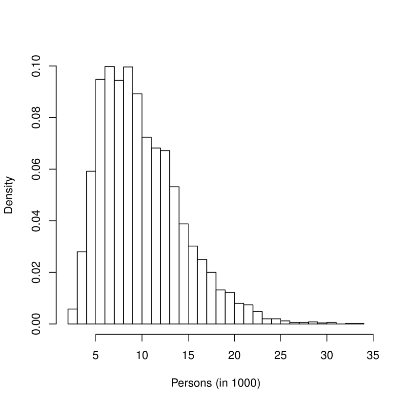
Again, the enormous difference between males and females becomes obvious. While 50.1 thousand females are affected in England and Wales (interquartile range (IQR): 40.3–60.9), for males the corresponding number is 9.2 (IQR: 6.6–12.5) thousand.

In situation described here, it is possible to derive the mean duration $\mathfrak{D}$ of SLE in males and females. The mean duration $\mathfrak{D}$ is the number of person-years of all SLE patients divided by the total number of persons who ever got it:

$$\mathfrak{D}=\frac{\sum\limits_{a=0}^{90}p(a)\cdot N(a)}{\sum\limits_{a=0}^{90}i(a)\cdot\bigl{(}1-p(a)\bigr{)}\cdot N(a)}.$$ (6)

If we calculate this value for all paths $p$, we find that in males and females the mean duration is 23.2 (IQR: 16.7–31.5) and 23.9 (IQR: 16.2–29.1) years, respectively. Thus, genders do not differ much in that respect. Similarly, the mean age at onset $\mathfrak{M}$ may be computed:

$$\mathfrak{M}=\frac{\sum\limits_{a=0}^{90}a\cdot i(a)\cdot\bigl{(}1-p(a)\bigr{)}\cdot N(a)}{\sum\limits_{a=0}^{90}i(a)\cdot\bigl{(}1-p(a)\bigr{)}\cdot N(a)}.$$ (7)

The empirical distribution of $\mathfrak{M}$ in the 5000 paths yields 51.750 (IQR: 51.748–51.752) and 46.108 (46.102–46.113) years in males and females, respectively. It is striking that $\mathfrak{M}$ has a relativly low variability in both genders. This is due to the factor $1-p(a)$, which is close to unity.

4 Conclusion

In the domain of infectious diseases, the theory of deterministic differential equations was generalized towards stochastic differential equations more than a decade ago, (Allen, 1999). In this article this transformation has been accomplished in the field of chronic diseases. The numbers of healthy and diseased persons have been modeled by a new system of two Îto stochastic differential equations. In rare chronic diseases such as systemic lupus erythematosus, a stochastic formulation might be preferable over a deterministic. Even if the incidence and mortality rates are well-known, statistical fluctuations in the number of diseased have a strong impact in the age course of the prevalence. This becomes obvious in Figures 6 and 6 where the distribution of the total number of males and females with SLE in England and Wales in 1995 have been estimated. The middle fifty spans about 6 and 20 thousand males and females respectively. Additionally, other disease characteristics have been calculated. The mean age at onset as derived in our theoretical model is 51.8 and 46.1 for males and females, respectively. The corrsponding empirical values 52.2 and 46.3 observed in the register data by Somers et al. are in good agreement. Another hint for the appropriateness of the methods described here comes from the basic epidemiological equation, that overall prevalence equals the product of overall incidence and duration of the disease (Szklo and Nieto, 2007). The overall prevalence in males and females can easily be obtained by Eq. (5) and the age pyramid $N(a)$. In our model the overall prevalence divided by the mean duration (Eq. (6)) yields the overall incidence $1.58$ and $7.95$ per 100000 person-years for males and females, respectively. Again, this is close to the empirically observed values $1.60$ and $8.01$ per 100000 person-years (Somers et al., 2007, Tab. 1). When relating the results of this study to other epidemiological data from the UK, especially the overall incidence for females appears high. Hopkinson et al. find a value of about $6.5$ per 100000 person-years only (1993). However, it has to be noted that the data of (Hopkinson et al., 1993) are in a way inconsistent: If we calculate the mean duration of SLE in females by the basic epidemiological equation for the data of Hopkinson et al., we find a mean duration of about 7 years only, which contradicts common survival times of persons with SLE (Cervera et al., 2003).

Although there is an ongoing debate about the differences between childhood-onset SLE and adult-onset as well as duration of SLE as a risk factor for comorbidities and mortality, it has to be noticed that reliable epidemiologic data about age at onset, duration of the disease, mean age of diseased etc are sparse or lacking. As an example, the sytematic review (Danchenko et al., 2006) about the global burden and epidemiology of SLE just found one study from Germany, the European country with the most inhabitants. The associated publication (Zink et al., 2001) was about prevalent cases, but did not mention a prevalence estimate. Incidence had not been adressed.

Theoretical models such as the one presented here may help to at least roughly estimate the burden and characteristics of rare chronic diseases. This is especially true in countries with few epidemiological or administrative data. However, the approach described here has several limitations. First, the stochastic differential equation (4) does not take into account calendar time trends. In the application to SLE, it has been shown that relative mortality of SLE patients undergoes a secular trend, (Bernatsky et al., 2006, Tab. 6). In the same publication we find, that relative mortality in persons with SLE depends on the duration of the disease. The longer a person is diseased, the more the relative risk decreases. Duration dependence is not modeled in Eq. (4). Hence, the new approach may be used as an approximation only, and more evaluations of the method are necessary to examine validity and applicability of the model. However, the disease characteristics derived by the new methods in this work are consistent and indicate an interesting and maybe fruitful way to go.

References

- Allen (1999) Allen EJ (1999). Stochastic Differential Equations and Persistence Time for two interacting populations. Dyn Contin Discrete Impulsive Syst 5 271–281
- Allen (2008) Allen LJS (2008). An Introduction to Stochastic Epidemic Models. In: Brauer F, Van den Driessche P, Wu J (ed.) Mathematical Epidemiology. Berlin: Springer, 81–130.
- Bernatsky et al. (2006) Bernatsky S, Boivin JF, Joseph L et al. (2006). Mortality in Systemic Lupus Erythematosus. Arthrit Rheumat 54 (8) 2550–2557
- Brinks (2011) Brinks R (2011). A new method for deriving incidence rates from prevalence data and its application to dementia in Germany. arXiv:1112.2720
- Cervera et al. (2003) Cervera R, Khamashta MA, Font J et al. (2003). Morbidity and mortality in systemic lupus erythematosus during a 10-year period: a comparison of early and late manifestations in a cohort of 1,000 patients. Medicine (Baltimore) 82 (5) 299–308
- Danchenko et al. (2006) Danchenko N, Satia JA, Anthony MS (2006). Epidemiology of systemic lupus erythematosus: a comparison of worldwide disease burden. Lupus 15 (5) 308–318.
- Darroch and Seneta (1967) Darroch JN, Seneta E (1967). On quasi-stationary distributions in absorbing continuous-time finite Markov chains. J Appl Probab 4 192–196
- Hopkinson et al. (1993) Hopkinson ND, Doherty M, Powell RJ (1993). The prevalence and incidence of systemic lupus erythematosus in Nottingham, UK, 1989-1990. Br J Rheumatol 32 (2) 110–115
- Kalbfleisch and Prentice (2002) Kalbfleisch JD, Pentice RL (2002). The Statistical Analysis of Failure Time Data. 2nd ed. Hoboken, NJ: Wiley.
- Kloeden and Platen (1999) Kloeden PE, Platen E (1999). Numerical Solution of Stochastic Differential Equations. Berlin: Springer
- Livingston et al. (2011) Livingston B, Bonner A, Pope J (2011). Differences in clinical manifestations between childhood-onset lupus and adult-onset lupus: a meta-analysis. Lupus 20 (13) 1345–1355
- Murray and Lopez (1994) Murray, CJL, Lopez AD (1994). Quantifying disability: data, methods and results Bulletin WHO 72 (3) 481–494
-
Office for National Statistics (2011)
Office for National Statistics (2011). Population Estimates Quinary Age Groups for
UK Constituent Countries – Mid-1971 to Mid-2010, updated on December 21st, 2011
http://www.ons.gov.uk, accessed January 12th, 2012 - Somers et al. (2007) Somers EC, Thomas SL, Smeeth L, Schoonen WM, Hall AJ (2007). Incidence of systemic lupus erythematosus in the United Kingdom, 1990–1999. Arthrit Care Res 57 (4) 612–618
- Szklo and Nieto (2007) Szklo M, Nieto FJ (2007). Epidemiology: Beyond the Basics. Sudbury, MA: Jones and Bartlett
- Zink et al. (2001) Zink A, Listing J, Klindworth C, Zeidler H (2001). The national database of the German Collaborative Arthritis Centres: Structure, aims, and patients. Ann Rheum Dis 60(3) 199–206