Chiral-mediated entanglement in an Aharonov-Bohm ring

Abstract

We study the orbital entanglement in a biased Aharonov-Bohm ring connected in a four-terminal setup. We find that the concurrence achieves a maximum when the magnetic flux $\Phi_{B}$ coincides with an integer number of half a flux quantum $\Phi_{0}/2$. We show that this behavior is a consequence of the existence of degenerate states of the ring having opposite chirality. We also analyze the behavior of the noise as a function of $\Phi$ and discuss the reliability of this quantity as an entanglement witness.

I INTRODUCTION

The increasing interest in quantum information processing is boosting the search for mechanisms to produce and control entanglement in devices of different nature. qe Photonic devices are routinely used for preparing and detecting entangled photon pairs.inter The main limitations of such devices is the non-existence of deterministic sources as well as the difficulty in controlling the interaction between the photons. Entanglement mechanisms have also been proposed in solid state devices, like quantum dots, entqdot and superconductors.entsup The fundamental ingredient behind all these mechanisms is a many-body interaction. More recently, it was determined that entanglement is also possible in systems of non-interacting electrons.been1 ; been2 In particular, it was shown that electron-hole entangled pairs can be produced by biasing a tunneling barrier.

The edge states of systems in the quantum Hall regime can be employed in solid state devices to produce electron beams with properties similar to those of a photon beam in optical setups. Exploiting this analogy, several theoretical and experimental proposals of electronic interferometers have been reported. elin Interestingly, the electronic counterpart of the Hanbury-Brown-Twiss device has been analyzed in a configuration of edge Hall states that do not have interfering orbits. hbt ; but1 For this reason, Aharonov-Bohm (AB) effect takes place only at the level of two-particle correlation functions, while the single-particle AB effect is not present. This entanglement seems to be related with an asymmetry in the device which favors the internal production of particle-hole pairs and manifest itself in the behavior of the current-current correlation functions. The relevance of the current-current correlation functions as entanglement witness has been also discussed in other fermionic systems. noise-ent

The aim of this work is to establish the existence of orbital entanglement in AB systems where single-particle interference is present. Using a microscopic model, we show that when coupling the AB-ring to four leads (two on the right and two on the left), the post select two-particle states of electrons at opposite leads are typically entangled. We name it ”chiral-mediated entanglement” (CME) because its creation is possible by the existence of intermediate states in the AB-ring which are coherent superpositions of two different chiralities for the electronic motion. Remarkably, this kind of entanglement can be also defined in a transport setup, which is identical to the one that was proposed to define the electron-hole entanglement, been1 ; been2 ; but1 ; but2 ; frust1 ; frust2 . In fact, we also show here that the noise current-current correlation function can be a good witness for the entanglement in our setup.

The paper is organized as follows. In Sec. II, we present the model in detail and we sketch the formulation of the theory, where we calculate the reduced density-matrix of a two-particle system. The results of this work are presented in Sec. III. The conclusions are presented in Sec. IV.

II THEORETICAL TREATMENT

II.1 Model

We consider the AB single-channel ring with a magnetic flux. The ring is connected to four terminals been1 ; been2 ; but1 ; but2 ; frust1 as shown in Fig. 1. Two of the terminals, those labeled by $\alpha=1,2$, at the left side of the ring, are at a higher voltage $V$ with respect to the ones at the right, labeled by $\alpha=3,4$. All terminals are ordinary single-channel metallic leads where electrons can move either to the right or to the left. For simplicity, we consider spinless electrons and we describe the setup by the Hamiltonian

$$H=\sum_{\alpha=1}^{4}\left(H_{\alpha}+H_{c,\alpha}\right)+H_{ring},$$ (1)

where $H_{\alpha}=\sum_{k_{\alpha}}\varepsilon_{k_{\alpha}}c^{\dagger}_{k_{\alpha}}c_{k_{\alpha}}$ are Hamiltonians of non-interacting electrons representing the leads. For the AB-ring we use a non-interacting model, where electrons move with velocity $v$ either clockwise ($+$ chirality) or anticlockwise ($-$ chirality). The Hamiltonian is

$$H_{ring}=\sum_{\lambda=\pm}\int_{0}^{L}dxv\lambda\Psi^{\dagger}_{\lambda}(x){\cal D}_{x}\Psi_{\lambda}(x),$$ (2)

being $\lambda$ the chirality, ${\cal D}_{x}=-i\partial_{x}-\phi,\;\;\phi=\Phi/(L\Phi_{0})$, with $\Phi=2\pi\Phi_{B}$, where $\Phi_{B}$ is the magnetic flux, $\Phi_{0}=hc/e$ is the flux quantum and $L$ is the length of the ring. The contacts between the leads and the ring are modeled by tunneling terms of the form $H_{c\alpha}=\sum_{k_{\alpha},\lambda=\pm}w_{k_{\alpha}}[c^{\dagger}_{k_{\alpha}}\Psi_{\lambda}(x_{\alpha})+H.c.]$, where $x_{\alpha}$ define the positions of the ring to which the leads are attached. We consider the leads to be at zero temperature. The chemical potentials enforce a bias voltage between left and right leads, i.e. $\mu_{1}=\mu_{2}=\mu_{L}$; $\mu_{3}=\mu_{4}=\mu_{R}$ and $\mu_{L}-\mu_{R}=eV$, which we assume to be very small $eV\sim 0$.

II.2 Reduced Density Matrix and Concurrence

In a setup as the one in Fig. 1, electrons tunnel from the left leads to the right ones. We aim to define the effective density matrix describing the quantum state post-selected from the total two–electron state by projecting out the components where both electrons are either in the right or in the left leads. been2 ; but2 ; frust1 We introduce the operators $A^{\dagger}_{00}\equiv c_{k_{1}}^{\dagger}c_{k_{3}}^{\dagger},A^{\dagger}_{01}\equiv c_{k_{1}}^{\dagger}c_{k_{4}}^{\dagger},A^{\dagger}_{10}\equiv c_{k_{2}}^{\dagger}c_{k_{3}}^{\dagger},A^{\dagger}_{11}\equiv c_{k_{2}}^{\dagger}c_{k_{4}}^{\dagger}$, which create one particle in one of the left leads and a second particle at one of the right leads. The ensuing the $4\times 4$ density matrix describes a system of two qubits with elements

$$[\rho^{(2)}(\varepsilon)]_{ab,a^{\prime}b^{\prime}} = \frac{1}{{\cal N}_{0}}\prod_{\alpha}\sum_{k_{\alpha}}\delta(\varepsilon-\epsilon_{k_{\alpha}})\langle A_{ab}^{\dagger}A_{a^{\prime}b^{\prime}}\rangle,$$

where ${\cal N}_{0}$ is a normalization factor, while the mean value is taken in the nonequilibrium state with a net current flowing from the left to the right. We remark that in our approach matrix elements of $\rho^{(2)}$ are obtained in terms of operators appearing in the Hamiltonian $H$. Expectation values of four time dependent creation and/or annihilation operators are computed using the nonequilibrium Green function formalism and Wick theorem, jauho

$$\langle c_{k_{\alpha}}^{\dagger}(t)c_{k_{\beta}}^{\dagger}(t)c_{k_{\lambda}}(t)c_{k_{\delta}}(t)\rangle=\int_{-\infty}^{\infty}d\varepsilon\int_{-\infty}^{\infty}d\varepsilon^{\prime}\left[G_{k_{\lambda},k_{\alpha}}^{<}(\varepsilon-\varepsilon^{\prime})G_{k_{\delta},k_{\beta}}^{<}(\varepsilon^{\prime})-G_{k_{\delta},k_{\alpha}}^{<}(\varepsilon-\varepsilon^{\prime})G_{k_{\lambda},k_{\beta}}^{<}(\varepsilon^{\prime})\right],$$ (3)

where $G_{k_{\alpha},k_{\beta}}^{<}(\varepsilon)$ is the Fourier transform with respect to $t-t^{\prime}$ of the lesser Green function

$$G_{k_{\alpha},k_{\beta}}^{<}(t-t^{\prime})=i\langle c_{k_{\beta}}^{\dagger}(t^{\prime})c_{k_{\alpha}}(t)\rangle.$$ (4)

We assume that $eV\sim 0$ and we are interested in analyzing $\varepsilon\sim\mu=(\mu_{L}+\mu_{R})/2$. We present the corresponding expression of $\rho^{(2)}$ in Appendix A.

From the above density matrix we compute the concurrence, which is a good measure of entanglement. woot In this case it is given by

$$\mathcal{C}\left[\rho^{(2)}\right]=max\left\{0,\sqrt{\lambda_{1}}-\sqrt{\lambda_{2}}-\sqrt{\lambda_{3}}-\sqrt{\lambda_{4}}\right\},$$ (5)

where $\lambda_{i}$ are the eigenvalues of $R:=\rho^{(2)}\sigma_{y}\bigotimes\sigma_{y}\rho^{(2)\ast}\sigma_{y}\bigotimes\sigma_{y}$ in decreasing order. It is interesting to notice that the concurrence so calculated is equivalent to the one obtained by the spin–dependent scattering formalism for a single mode conductor ,been1 ; been2 which is

$$\mathcal{C}=2\frac{\sqrt{\tau_{1}(1-\tau_{1})\tau_{2}(1-\tau_{2})}}{\tau_{1}+\tau_{2}-\tau_{1}\tau_{2}}.$$ (6)

Here, $\tau_{1},\tau_{2}$ are transmission eigenvalues of the scattering matrices $s_{\alpha,\beta}(\mu)=\delta_{\alpha,\beta}-i\sqrt{\Gamma_{\beta}\Gamma_{\alpha}}G_{\alpha,\beta}^{R}(\mu)$, where $G_{\alpha,\beta}^{R}(\mu)$ is the Fourier transform with respect to $t-t^{\prime}$ of the retarded Green function

$$G_{\alpha,\beta}^{R}(t-t^{\prime})=-i\Theta(t-t^{\prime})\sum_{\lambda,\lambda^{\prime}}\langle\{\Psi_{\lambda}(x_{\alpha},t),\Psi^{\dagger}_{\lambda^{\prime}}(x_{\beta},t^{\prime})\}\rangle$$ (7)

evaluated at $\mu$, being $x_{\alpha}$ the position of the ring at which the wire $\alpha$ is attached. while $\Gamma_{\alpha}=2\pi\sum_{k_{\alpha}}w_{k_{\alpha}}^{2}\delta(\mu-\varepsilon_{k_{\alpha}})$. fish-lee

II.3 Noise

As pointed out in Refs. been2, ; frust2, the concurrence can be expressed in terms of correlators that quantify the degree of violation of Bell inequalities. In transport setups the latter can in turn be directly related to current-current correlation functions, which are amenable to be experimentally detected. We, thus, turn to analyze the connection between these correlation functions and the above discussed entanglement. We first outline the procedure to compute the current-current noise within our treatment. The current passing through the contact to the terminal $\alpha$, can be expressed by the following operator $J_{\alpha}(t)=(e/\hbar)\sum_{k_{\alpha}}w_{k_{\alpha}}[ic_{k_{\alpha}}^{\dagger}(t)\Psi(x_{\alpha},t)+h.c]$. The zero frequency shot-noise is a measure of the current-current correlations in different terminals. It reads

$${\cal S}_{\alpha,\beta}(0)=\frac{1}{2}\int d\tau\langle\{\delta J_{\alpha}(\tau),\delta J_{\beta}(0)\}\rangle,$$ (8)

where $\delta J_{\alpha}=J_{\alpha}-\langle J_{\alpha}\rangle$. We calculate (ec.(8)) by evaluating a bubble diagram in terms of nonequilibrium Green functions. The corresponding expressions are presented in Appendix B. Shot Noise Calculation.

III RESULTS

III.1 Qualitative Analysis

To understand the origin of CME it is useful to begin analyzing the electronic states of the isolated AB–ring. The Hamiltonian can be diagonalized in momentum space: Defining $\Psi_{\lambda}(x)=1/\sqrt{{\cal N}}\sum_{p}e^{-ipx}c_{p,\lambda}$ with ${\cal N}$ a normalization factor, $p=2\pi n/L$ and $n\in\mathbf{Z}$ we obtain $H_{ring}=\sum_{\lambda}\sum_{p}\varepsilon_{p,\lambda}(\Phi)c^{\dagger}_{p,\lambda}c_{p,\lambda}$, with $\varepsilon_{p,\lambda}=\lambda v(p-\phi)$ (a cutoff in the single- particle energy spectrum is assumed). The effect of the magnetic flux on the energies $\varepsilon_{p,\lambda}(\Phi)$ is illustrated in Fig. 1. Depending on the magnetic flux, there can be zero, one or two single-particle states $|p,\lambda\rangle$ with a given energy. States with different chirality $\lambda=\pm$ are degenerate only when the flux is an integer multiple of $\pi\Phi_{0}$.

Let us consider first the case where two degenerate states with opposite chiralities exist in the ring. These two states behaves as an intermediate qubit that couples to the qubits defined by the leads. We will argue that in this case CME naturally emerges between electrons at the right and left leads. The $N$-particle states with a Fermi energy $\epsilon_{F}$ can be obtained from $|\overline{0}\rangle$, that represents the Fermi sea with $N-2$ particles filling the states with $\varepsilon_{p,\lambda}(\Phi)<\epsilon_{F}$, where $v(p_{F}-\phi)=\epsilon_{F}$. Thus, we have $|\Psi_{ring}\rangle=c^{\dagger}_{p_{F},+}c^{\dagger}_{p_{F},-}|\overline{0}\rangle$. When the ring is in contact with the four leads, particles can tunnel between the ring and the reservoirs. For weak coupling we can assume that each of the chiral levels with $p_{F}$ hybridize with the levels of the leads having the same energy $\epsilon_{F}$. This is described by the following effective Hamiltonian

$$H_{eff}=w\sum_{\alpha=1}^{4}\sum_{\lambda=\pm}e^{i\lambda p_{F}x_{\alpha}}[c^{\dagger}_{k_{\alpha}}c_{p_{F},\lambda}+H.c.],$$ (9)

where $w$ is the effective tunneling parameter, $c^{\dagger}_{k_{\alpha}}$ creates an electron in the single-particle state of the $\alpha$-lead with energy $\varepsilon_{k_{\alpha}}=\epsilon_{F}$ (we take $\epsilon_{F}=0$ without loss of generality). This Hamiltonian has four eigenstates of the form

$$|\psi_{n}\rangle=[\sum_{\alpha=1}^{4}\gamma_{n,\alpha}c^{\dagger}_{k_{\alpha}}+\sum_{\lambda=\pm}\gamma_{n,\lambda}c^{\dagger}_{p_{F},\lambda}]|0\rangle,\;\;\;\;n=1,\ldots,4,$$ (10)

where the coefficients $\gamma_{n}$ are the weights of the eigenstates in the chosen base. It also has two additional degenerate states of the form $|\psi_{n}\rangle=\sum_{\alpha=1}^{4}\gamma_{n,\alpha}c^{\dagger}_{k_{\alpha}}|0\rangle,\;n=5,6$. The latter correspond to states that do not hybridize with the ring. When two particles are present, two different such states must be occupied. It is simple to show that any state of this type has a sizable projection on states of the form $\sum_{\alpha\neq\beta}\Lambda_{\alpha,\beta}c^{\dagger}_{k_{\alpha}}c^{\dagger}_{k_{\beta}}|0\rangle$ for some non-vanishing coefficients $\Lambda_{\alpha,\beta}$. This two-particle state is typically entangled in the orbital indices $\alpha,\beta$ of opposite leads. Notice that it is also possible to use two AB–rings with degenerate levels as a two-qubit system coupled by two conducting leads (intermediate qubit).

On the other hand if we consider the case of a one chirality ring ($\epsilon_{p}=v(p-\phi)$ for example) the situation drastically changes and no significant entanglement between left and right leads is attained. This is can be seen because the effective Hamiltonian has a different level structure. In fact, $H_{eff}$ can be naturally written in terms of operators that are linear combinations of the lead operators $c^{\dagger}_{k_{\alpha}}$ as $H_{eff}=w(f^{\dagger}c_{p_{F},\lambda}+H.c.)$, with $f^{\dagger}=(1/2)\sum_{\alpha=1}^{4}e^{ip_{F}x_{\alpha}}c^{\dagger}_{k_{\alpha}}$, while there are three additional orthogonal linear combinations of these operators which do not hybridize with the ring. The two eigenstates of $H_{eff}$ are linear combinations of a single-particle state of the leads and a single-particle state of the ring. Thus, a two-particle state of this Hamiltonian has never the two particles in the leads and therefore no orbital entanglement is possible.

The above argument suggests that by varying the magnetic flux, or the chemical potential of the leads (or equivalently, a gate voltage applied at the ring) we can induce the system to switch from a situation with no orbital entanglement between the leads onto another situation with inter-lead entanglement. This is done by varying $\Phi$ and/or $\mu$ in order to have degenerate chiral states of the ring at the Fermi energy. We now present a rigorous calculation of the entanglement for the states that are relevant for a transport experiment in the coherent regime and explain how the CME depends on flux and chemical potential. We also discuss the way in which it may be detected in transport experiments.

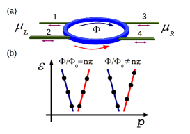
Figure 1: (a) Scheme of an Aharonov-Bohm ring with two chiralities, attached to four leads. The chemical potentials are such that there is a bias voltage between the left and right leads. Electrons incoming from the left can tunnel to the ring and escape through leads. (b) Linear dispersion relation of an isolated AB-ring, where electrons move with velocity $v$ either clockwise ($+$ chirality) or anticlockwise ($-$ chirality). The magnetic flux determines whenever the Fermi level is two-degenerate or not.

III.2 Numerical Results

III.2.1 Concurrence

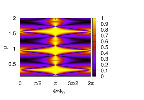
Figure 2: (Color online) Concurrence as a function of $\Phi/\Phi_{0}$ and mean chemical potential $\mu$ for a ring with length $L=20$ with wires connected at $x_{1}=1,\;x_{2}=6,x_{3}=11,x_{4}=16$.

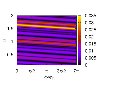
Figure 3: (Color online) Concurrence as a function of $\Phi/\Phi_{0}$ and mean chemical potential $\mu$ for a ring with only one chirality. The ring parameters are the same as in Fig.2.

The behavior of $\mathcal{C}$ as a function of the mean chemical potential $\mu$ and the magnetic flux $\Phi$ is shown in Fig. 2. The concurrence is maximal at $\Phi/\Phi_{0}=n\pi$ and for values $\mu$ close to the energy of two degenerate chiral states of the ring. The same type of behavior is observed for other configurations of the wires, corresponding to contacts at different positions $x_{\alpha}$. For this Fig. we considered wires with a bandwidth $W_{\alpha}$ and $\Gamma_{\alpha}=\Omega_{\alpha}\sqrt{W_{\alpha}^{2}-\mu^{2}}$, where $\Omega_{\alpha}$ is a constant, but the same behavior is obtained for leads with a constant density of states. For some chemical potentials ${\cal C}$ exhibits maxima at $\Phi/\Phi_{0}=0,\mod(2\pi)$, which corresponds to the energy of two degenerate states of the ring, but achieves again the maximum value within a wide range of fluxes centered at $\Phi/\Phi_{0}=\pi,\mod(2\pi)$. This feature is analyzed below in more detail.

Instead, if we evaluate ${\cal C}$ for the Hamiltonian (2) restricted to a single chirality, we find negligibly orbital entanglement in the leads within the whole range of $\Phi$ and $\mu$. These results are presented in Fig.3. In this case the ring behaves as a single-level system, and prevent the formation of orbital entangled states at the leads.

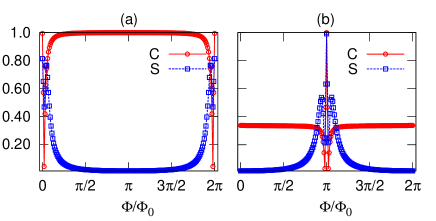
Figure 4: (Color online) Shot noise (squares) between left and right terminals, as a function of $\Phi/\Phi_{0}$ for two values of the chemical potentials at which there are degenerate states. (a) $\mu=0.3175$, (b) $\mu=0.7866$. The corresponding plots for the concurrence are also shown for comparison (circles).

III.2.2 Noise

We now turn to present results on the behavior of the current-current correlation functions. Our aim is to analyze if the signatures of entanglement found in the behavior of the concurrence can be also identified in the behavior of the noise. Results for the total left-right noise correlations $S=\sum_{\alpha=1,2,\beta=3,4}{\cal S}_{\alpha,\beta}(0)$ (equal to the self-correlation $-\sum_{\alpha,\beta=1,2}{\cal S}_{\alpha,\beta}(0)$ ) are shown in Fig. 4. The left (right) panel, corresponds to a chemical potential $\mu$ for which there are two degenerate chiral states in the ring for $\Phi/\Phi_{0}=0,(\pi),\mbox{mod}(2\pi)$. The behavior of the concurrence is also plotted for comparison. In both cases, $S$, along with ${\cal C}$ exhibit maxima at the fluxes for which the two degenerate chiral states are resonant at the given $\mu$. This points to the idea that noise is indeed a reliable witness of orbital entanglement, as discussed in the context of other electronic setups. been1 ; been2 ; but1 ; noise-ent In the case of the left panel, both quantities are maximum at $\Phi/\Phi_{0}=0,\mbox{mod}(2\pi)$. Within a range of fluxes which scans the width of the resonant degenerate levels of the ring they first decrease and then increase, displaying a dip. As the flux increases further, the behavior of these two quantities, however, depart one another. While $S$ tends to vanish around $\Phi/\Phi_{0}=\pi$, the concurrence displays a wide plateau with height ${\cal C}\sim 1$. Qualitatively, the same type of behavior is observed in the right panel. In this case, both quantities exhibit a sharp maxima at resonance (see the peaks around $\Phi/\Phi_{0}=\pi$). The concurrence displays a plateau and another (lower) maximum around $\Phi/\Phi_{0}=0,\mbox{mod}(2\pi)$ while $S$ is vanishing small. On general grounds this is rather surprising, since one could easily imagine situations with a sizable noise without entanglement, but here we have the converse situation.

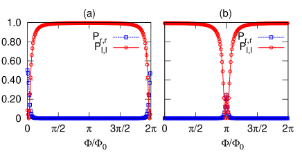
Figure 5: (Color online) Probability of finding two particles at the left and right leads as a function of magnetic flux $\Phi/\Phi_{0}$. Panels (a) and (b) correspond to the same parameters of Fig. 4 (a) and (b), respectively .

In order to further understand the relation between the behavior of ${\cal C}$ and $S$ as well as the connection to the CME, we analyze the probabilities

$$P_{LL} = \prod_{\alpha}\sum_{k_{\alpha}}\delta(\varepsilon-\epsilon_{k_{\alpha}})\langle c^{\dagger}_{k_{1}}c_{k_{1}}c^{\dagger}_{k_{2}}c_{k_{2}}\rangle,$$

$$P_{RR} = \prod_{\alpha}\sum_{k_{\alpha}}\delta(\varepsilon-\epsilon_{k_{\alpha}})\langle c^{\dagger}_{k_{3}}c_{k_{3}}c^{\dagger}_{k_{4}}c_{k_{4}}\rangle$$ (11)

of finding two particles at the left (right) leads, respectively. In Fig. 5 we show the behavior of these two quantities for the same parameters of Fig. 4. It is clear that $P_{LL}$ and $P_{RR}$ are both sizable when tunneling through the ring is allowed. For these chemical potentials, this corresponds to the narrow window of fluxes around $\Phi/\Phi_{0}=0(\pi)$, for the case of the left (right) panels, respectively, within which the degenerate levels of the ring remain resonant. Beyond these values, the transmission from left to right is blocked and the two particles have a high probability of remaining within the left wires. A further analysis of Figs. 2 and 4 in the light of the results shown in Fig. 5, then reveals that the high values of concurrence in the plateaus away from $\Phi/\Phi_{0}=0(\pi),\mbox{mod}(2\pi)$ in the case of the left (right) panels of Fig. 4, correspond to states which have a very low probability of taking place. Instead, the resonant situation with two degenerate chiral states of the ring at the Fermi energy, leads to a high orbital entanglement which is clearly witnessed by a high noise amplitude $S$.

IV CONCLUSION

To summarize, we introduced a new mechanism for orbital entanglement. This type of entanglement is originated in the spectral nature of the AB ring and is highly sensitive to the magnetic field. Orbitally entangled electronic pairs can be produced by suitably tuning the magnetic field, the chemical potential or a voltage gate at the ring, in order to have a degenerate pair of electronic states with different chiralities at the Fermi energy (intermediate qubit). In fact, if the right and left leads are mediated by a single–level system (single-chirality ring) the orbital entanglement is negligible. This type of entanglement can be detected in transport experiments, the shot noise being a good witness. The setup of Fig. 1 could be experimentally realized in an architecture based on the quantum Hall regime of a 2D electron gas, by substituting each wire by a pair of incoming and outgoing edge states and the ring by a pair of edge states with different chiralities, separated by a narrow circular wall. In such a setup it would be possible to combine the main system of Fig. 1 with beam splitters connected at the wires, in order to test Bell inequalities and even perform the full quantum tomography following the protocol of Ref. but2, . Two interesting possible generalizations are the combination between static and flying qubits by combining with quantum dots, schom as well as the introduction of dynamical single-particle emitters at the sources.spe

APPENDIX

A. Reduced Density Matrix

We evaluate the post-selected state of two electrons at opposite leads, $\rho^{(2)}$, in terms of Green functions (the Fourier transform of ec.(7)). The explicit expression of a general matrix element, up to a normalization factor, is:

$$\prod_{\nu=1}^{4}\sum_{k_{\nu}}\delta(\varepsilon-\epsilon_{k_{\nu}})\langle c_{k_{\alpha}}^{\dagger}(t)c_{k_{\beta}}^{\dagger}(t)c_{k_{\lambda}}(t)c_{k_{\delta}}(t)\rangle=\Gamma^{2}\left[f_{\alpha}(\varepsilon)f_{\beta}(\varepsilon)G_{{}_{\lambda},_{\alpha}}^{R}(\varepsilon)G_{{}_{\delta},_{\beta}}^{R}(\varepsilon)-f_{\alpha}(\varepsilon)f_{\delta}(\varepsilon)G_{{}_{\lambda},_{\alpha}}^{R}(\varepsilon)G_{{}_{\delta},_{\beta}}^{A}(\varepsilon)\right.$$

$$\left.-f_{\lambda}(\varepsilon)f_{\beta}(\varepsilon)G_{{}_{\delta},_{\beta}}^{R}(\varepsilon)G_{{}_{\lambda},_{\alpha}}^{A}(\varepsilon)\right]-i\sum_{\gamma=1}^{4}\Gamma^{3}\left[f_{\beta}(\varepsilon)f_{\gamma}(\varepsilon)G_{{}_{\lambda},_{\gamma}}^{R}(\varepsilon)G_{{}_{\delta},_{\beta}}^{R}(\varepsilon)G_{{}_{\gamma},_{\alpha}}^{A}(\varepsilon)\right.$$

$$\left.f_{\alpha}(\varepsilon)f_{\gamma}(\varepsilon)G_{{}_{\lambda},_{\alpha}}^{R}(\varepsilon)G_{{}_{\delta},_{\gamma}}^{R}(\varepsilon)G_{{}_{\gamma},_{\beta}}^{A}(\varepsilon)\right]+\sum_{\gamma,\eta=1}^{4}\Gamma^{4}f_{\eta}(\varepsilon)f_{\gamma}(\varepsilon)G_{{}_{\lambda},_{\gamma}}^{R}(\varepsilon)G_{{}_{\delta},_{\eta}}^{R}(\varepsilon)G_{{}_{\eta},_{\beta}}^{A}(\varepsilon)G_{{}_{\gamma},_{\alpha}}^{A}(\varepsilon)$$

$$+\Gamma\left[-if_{\alpha}(\varepsilon)f_{\beta}(\varepsilon)G_{{}_{\delta},_{\beta}}^{R}(\varepsilon)+if_{\alpha}(\varepsilon)f_{\delta}(\varepsilon)G_{{}_{\delta},_{\beta}}^{A}(\varepsilon)-\Gamma\sum_{\gamma=1}^{4}f_{\gamma}(\varepsilon)f_{\alpha}(\varepsilon)G_{{}_{\delta},_{\gamma}}^{R}(\varepsilon)G_{{}_{\gamma},_{\beta}}^{A}(\varepsilon)\right]\delta_{k_{\alpha},k_{\lambda}}$$

$$+\Gamma\left[-if_{\delta}(\varepsilon)f_{\alpha}(\varepsilon)G_{{}_{\lambda},_{\alpha}}^{R}(\varepsilon)+if_{\lambda}(\varepsilon)f_{\delta}(\varepsilon)G_{{}_{\lambda},_{\alpha}}^{A}(\varepsilon)-\Gamma\sum_{\gamma=1}^{4}f_{\gamma}(\varepsilon)f_{\delta}(\varepsilon)G_{{}_{\lambda},_{\gamma}}^{R}(\varepsilon)G_{{}_{\gamma},_{\alpha}}^{A}(\varepsilon)\right]\delta_{k_{\delta},k_{\beta}}$$

$$-\sum_{k_{\alpha}}\sum_{k_{\delta}}\delta(\varepsilon-\epsilon_{k_{\alpha}})\delta(\varepsilon-\epsilon_{k_{\delta}})f_{\delta}(\varepsilon)f_{\alpha}(\varepsilon)\delta_{k_{\alpha},k_{\lambda}}\delta_{k_{\delta},k_{\beta}},$$ (12)

where we considered all spectral densities equal $\Gamma_{\alpha}=\Gamma$ $\forall\alpha$. $f_{\alpha}(\varepsilon)$ is de Fermi distribution function of the lead $\alpha$. Note that $G_{\alpha,\beta}^{R}(\varepsilon)=\sum_{\lambda,\lambda^{\prime}}G_{\lambda,\lambda^{\prime}}^{R}(x_{\alpha},x_{\beta},\varepsilon)$.The retarded Green functions are evaluated by solving the Dyson equation,

$$G^{R}_{\lambda,\lambda^{\prime}}(x,x^{\prime},\varepsilon)=g^{R}_{\lambda^{\prime}}(x,x^{\prime},\varepsilon)\delta(x-x^{\prime})\delta_{\lambda,\lambda^{\prime}}+\sum_{\gamma=1}^{4}\sum_{\lambda^{\prime\prime}}G^{R}_{\lambda,\lambda^{\prime\prime}}(x,x_{\gamma},\varepsilon)\Sigma_{\gamma}^{R}(\varepsilon)g^{R}_{\lambda^{\prime}}(x_{\gamma},x^{\prime},\varepsilon),$$ (13)

being

$$g^{R}_{\lambda^{\prime}}(x,x^{\prime},\varepsilon)=\frac{1}{\mathcal{M}}\sum_{k=-k_{0}}^{k_{0}}\frac{e^{-ik(x-x^{\prime})}}{\varepsilon-\varepsilon_{k,\lambda^{\prime}}(\Phi)+i\eta},$$ (14)

where $k_{0}$ is the energy cut off and $\mathcal{M}=2k_{0}+1$ a normalization factor, the uncoupled retarded Green function of the ring and $\Sigma_{\gamma}^{R}(\varepsilon)=\sum_{k_{\alpha}}|w_{k_{\alpha}}|^{2}g_{k_{\alpha}}^{R}(\varepsilon)$ the self energy of reservoir $\alpha$.

B. Shot Noise Calculation

Here we show the shot noise expression of ec.(8) in terms of retarded Green functions. jauho

$$S_{\alpha,\beta}(0) =\frac{1}{2}\int d\tau\left[\langle\{J_{\alpha}(\tau),J_{\beta}(0)\}\rangle-2\langle J_{\alpha}(\tau)\rangle\langle J_{\beta}(0)\rangle\right]$$

$$=\frac{e^{2}}{2\hbar}\int\frac{d\varepsilon}{2\pi}\lgroup\sum_{\delta,\gamma=1}^{4}\left[\Gamma_{\alpha}\Gamma_{\beta}\Gamma_{\delta}\Gamma_{\gamma}[(1-f_{\gamma}(\varepsilon))f_{\delta}(\varepsilon)+(1-f_{\delta}(\varepsilon))f_{\gamma}(\varepsilon)]G_{\beta,\gamma}^{R}(\varepsilon)G_{\alpha,\gamma}^{R*}(\varepsilon)G_{\alpha,\delta}^{R}(\varepsilon)G_{\beta,\delta}^{R*}(\varepsilon)\right]$$

$$-2\Gamma_{\alpha}\Gamma_{\beta}[(1-f_{\beta}(\varepsilon))f_{\alpha}(\varepsilon)+(1-f_{\alpha}(\varepsilon))f_{\beta}(\varepsilon)]\mathcal{R}e\{G_{\alpha,\beta}^{R}(\varepsilon)G_{\beta,\alpha}^{R}(\varepsilon)\}$$

$$-2\Gamma_{\alpha}\Gamma_{\beta}\mathcal{R}e\{iG_{\beta,\alpha}^{R}(\varepsilon)\sum_{\delta=1}^{4}G_{\alpha,\delta}^{R}(\varepsilon)G_{\beta,\delta}^{R*}(\varepsilon)\Gamma_{\delta}\left[(1-f_{\alpha}(\varepsilon))f_{\delta}(\varepsilon)+(1-f_{\delta}(\varepsilon))f_{\alpha}(\varepsilon)\right]\}$$

$$-2\Gamma_{\alpha}\Gamma_{\beta}\mathcal{R}e\{iG_{\alpha,\beta}^{R}(\varepsilon)\sum_{\delta=1}^{4}G_{\beta,\delta}^{R}(\varepsilon)G_{\alpha,\delta}^{R*}(\varepsilon)\Gamma_{\delta}\left[(1-f_{\beta}(\varepsilon))f_{\delta}(\varepsilon)+(1-f_{\delta}(\varepsilon))f_{\beta}(\varepsilon)\right]\}$$

$$+2\delta_{\alpha,\beta}\Gamma_{\alpha}\sum_{\delta=1}^{4}\Gamma_{\delta}|G_{\alpha,\delta}^{R}(\varepsilon)|^{2}\left[(1-f_{\delta}(\varepsilon))f_{\alpha}(\varepsilon)+(1-f_{\alpha}(\varepsilon))f_{\delta}(\varepsilon)\right]\rgroup.$$

References

- (1) R. Horodecki et al, Rev. Mod. Phys. 81, 865-942 (2009).
- (2) R. Hanbury Brown and R. Q. Twiss, Nature 178 , 1046 (1956); C. K. Hong, Z. Y. Ou, and L. Mandel, Phys. Rev. Lett. 59, 2044 (1987).
- (3) D. Loss and D. P. DiVincenzo, Phys. Rev. A 57, 120 (1998); R. Hanson, L .P. Kouwenhoven, J. R. Petta, S. Tarucha, and L. M. K. Vandersypen, Rev. Mod. Phys. 79, 1217 (2007).
- (4) J. Wei, and V. Chandrasekhar, Nature Phys. 6, 494 (2010).
- (5) C. W. J. Beenakker, C. Emary, M. Kindermann, and J. L. van Velsen, Phys. Rev. Lett. 91, 147901 (2003).
- (6) C. W. J. Beenakker, in ”Quantum Computers, Algorithms and Chaos”, Proceedings of the International School of Physics E. Fermi, Varenna, 2005, (IOS Press, Amsterdam, 2006); C. W. J. Beenakker, M. Kindermann, C. M. Marcus, and A. Yacoby in ”Fundamental Problems of Mesoscopic Physics”, edited by I. V. Lerner, B. L. Altshuler and Y. Gefen, NATO Science Series II, vol 154 (Kluwer, Dordrecht, 2004).
- (7) M. Henny, S. Oberholzer, C. Strunk, T. Heinzel, K. Ensslin, M. Holland, and C. Schönenberger; Science 284, 296 (1999); W.D. Oliver, J. Kim, R.C. Liu, and Y. Yamamoto, ibid. 284, 299 (1999); H. Kiesel, A. Renz, and F. Hasselbach, Nature 418, 392 (2002); Y. Ji, Y. Chung, D. Sprinzak, M. Heiblum, D. Mahalu, and H. Shtrikman, Nature 422, 415 (2003); I. Neder, N. Ofek, Y. Chung, M. Heiblum, D. Mahalu, and V. Umansky, Nature 448, 333 (2007); V. Giovannetti, D. Frustaglia, F. Taddei, and R. Fazio, Phys. Rev. B 74, 115315 (2006).
- (8) I. Neder, N. Ofek, Y. Chung, M. Heiblum, D. Mahalu, V. Umansky, Nature 448, 333 (2007).
- (9) P. Samuelsson, E.V. Sukhorukov, M. Büttiker, Phys. Rev. Lett. 92, 026805 (2004).
- (10) P. Samuelsson, M. Büttiker, Phys. Rev. B 73, 041305 (2006).
- (11) I. Klich and L. Levitov, Phys. Rev. Lett. 102, 100502 (2009); B. Hsu, E. Grosfeld and E. Fradkin Phys. Rev. B 80, 235412 (2009).
- (12) V. A. Gopar, D. Frustaglia, Phys. Rev. B 77, 153403 (2008).
- (13) D Frustaglia and A. Cabello, Phys. Rev. B 80, 201312(R) (2009).
- (14) W. K. Wooters, Phys. Rev. Lett. 80, 2245 (1998).
- (15) H. J. W. Haug and A-P. Jauho, ”Quantum kinetics in transport and optics of semiconductors”, Springer (2008).
- (16) D. S. Fisher and P. A. Lee, Phys. Rev. B 23, 6851 (1981).
- (17) H. Schomerus, and J. P. Robinson, New J. Phys 9, 67 (2007).
- (18) G. Fève, A. Mahe, J.-M. Berroir, T. Kontos, B. Placais, DC Glattli, A. Cavanna, B. Etienne, Y. Jin, Science 316, 1169 (2007); J. Splettstoesser, M. Moskalets, M. Büttiker Phys. Rev. Lett. 103, 076804 (2009).