A hybrid approach to cosmic microwave background lensing reconstruction from all-sky intensity maps

On the basis of realistic simulations, we propose a hybrid method to reconstruct the lensing potential power spectrum, directly on PLANCK-like cosmic microwave background frequency maps. This involves the use of a large Galactic mask and the treatment of strong inhomogeneous noise. For $\ell\lesssim 100$, we show that a full-sky inpainting method, which was previously described, still allows a minimal variance reconstruction, with a bias that must be accounted for by a Monte Carlo method but that does not couple to the deflection field. For $\ell\gtrsim 100$, we develop a method based on tiling the cut-sky with local $10\degr\times 10\degr$ overlapping tangent planes (referred to in the following as patches). We tackle various issues related to their size/position, non-periodic boundaries, and irregularly sampled data of the planes after the sphere-to-plane projection. We show that the predominant noise term of the quadratic lensing estimator determined from an apodized patch can still be recovered directly from the data. To prevent any loss of spatial accuracy, we developed a tool that allows the efficient determination of the complex Fourier series coefficients from a bi-dimensional irregularly sampled dataset, without performing any interpolation. We show that our multi-patch approach enables the lensing power spectrum to be reconstructed with a very small bias, thanks to the omission of a Galactic mask and smaller noise inhomogeneities, as well as an almost minimal variance. At each stage the data quality can be assessed and simple bi-dimensional spectra compiled, which allows the control of local systematic errors.

Introduction

Experiments have now reached the sensitivity in terms of both resolution and noise, to detect the tiny deflection of the cosmic microwave background (CMB) photons ($\sigma_{d}\simeq 2.7\arcmin$) by the irregular distribution of matter, in their journey from the last scattering surface to Earth. First results on the power spectrum of this deflection field have been reported by the ACT (Das et al. 2011) and SPT (van Engelen et al. 2012) collaborations. The PLANCK spatial mission should soon provide firm measurements. This information provides access to a new cosmological observable that is sensitive to an epoch ($1\lesssim z\lesssim 3$) much more recent than the CMB decoupling one ($z\simeq 1100$), giving us a lever-arm to lift the so-called geometrical degeneracy (Stompor & Efstathiou 1999), but using one single consistent data-set. In particular, it probes the matter density fluctuations, on scales where the free-streaming of massive neutrinos significantly erases the power spectrum of these fluctuations (Lesgourgues & Pastor 2006), and is expected to help us to determine their total mass by means of global cosmological fits.

On statistical grounds, the properties of the (nearly) optimal quadratic estimator for lensing power reconstruction are now well-understood, both in the (infinite) flat sky limit and across the complete sphere (Hu & Okamoto 2002; Okamoto & Hu 2003).

However, real data are affected by contaminants, mostly Galactic dust and point sources in the case of CMB frequency maps, requiring a revised means of lensing reconstruction on a cut-sky, which is a non-trivial task. In addition, the scanning strategy of the specific instrument, particularly in the case of PLANCK, induces some strong spatial-noise inhomogeneities that are not taken into account in the classical estimator of lensing, and must be corrected for by Monte Carlo simulations. In the general case, both effects cannot be distinguished during the reconstruction process.

In a previous study (Perotto et al. 2010), we optimized a sparse inpainting procedure to restore the missing data inside the mask, without significantly biasing the lensing results. We however neglected the noise inhomogeneity. Furthermore, the work was oriented towards component-separated maps, so that the mask to be filled was rather small (about 10% of the sky).

However before having to adopt a component separation method that mixes different maps, we wish to investigate in this paper whether the lensing potential can be reconstructed more directly in individual intensity CMB maps, which is indeed a necessary step in assessing the possible systematic errors. For PLANCK, the channels under consideration correspond to 100, 143, and 217GHz (Planck Coll. 2005). This requires the treatment of much larger masks. We will also consider the strong spatial-noise inhomogeneities induced by the scanning strategy.

We revisit the sparse inpainting method in this new configuration (a $30\%$ mask + inhomogeneous noise) and show that i) the estimator under these conditions is strongly biased and ii) a Monte Carlo approach can be used to correct for this bias. We also propose an alternative method (multi-patch) that allows us to completely avoid the Galactic region, during the development of which we solved a number of issues related to the pixelized-sphere to plane projection.

After rapidly reviewing the various noise contributions to the quadratic estimator (QE) in Sect. 1, and the common simulations used in Sect. 2, we update our full-sky inpainting analysis (hereafter denoted FS-inpainting) in Sect. 3. Most of the paper in Sect. 4, then deals with resolving issues related to the projection of a non-periodic signal from a pixelized sky onto a local patch. In particular, we present a new algorithm (detailed in the Appendix) that allows a fast reconstruction of band-limited Fourier series coefficients from irregularly sampled data, without performing any interpolation. We then compare both methods, optimize the results in Sect. 5, and argue that a hybrid reconstruction is the most appropriate. In this hybrid approach, the full sky lensing reconstruction presented in Perotto et al. (2010) is used at low $\ell$, with an additive Monte Carlo bias correction, while at high $\ell$, the new multi-patch method is advocated.

This method allows the direct reconstruction of lensing signal from PLANCK-like CMB frequency maps (namely those at the 100, 143, and 217 GHz). While it would be premature to decide today whether performing a multi-map component separation provides a more accurate recovery of the lensing signal, we give some elements of the discussion in the conclusion.

1 A brief review of the quadratic estimator

The gravitational lensing potential $\phi$ is a scalar isotropic field (for a review, see e.g. Lewis & Challinor 2006) that spatially remaps the CMB photons according to

$$T(\@vec{n})=T_{\text{CMB}}(\@vec{n}+\@vec{d}(\@vec{n})),$$ (1)

where $\@vec{d}=\nabla\phi$ is the deflection field, which has a power spectrum on the sky $C_{\ell}^{d}=\ell(\ell+1)C_{\ell}^{\phi}$, or $C_{K}^{d}=k^{2}C_{K}^{\phi}$ in the flat sky limit. This process slightly breaks the Gaussianity of the CMB field, and estimators have been searched for in order to extract the lensing information using its very local properties

The quadratic estimator was proposed by Hu & Okamoto (2002). For CMB temperature anisotropies, it consists in taking the (weighted) convolution of the observed Fourier modes according to

$$\hat{\phi}(\@vec{K})=A_{K}\int\frac{d^{2}k_{1}}{(2\pi)^{2}}T(\@vec{k}_{1})T(\@vec{K}-\@vec{k}_{1})F(\@vec{k}_{1},\@vec{K}-\@vec{k}_{1}),$$ (2)

where the normalization $A_{K}$ and filter $F$ are determined by requiring the estimator to be un-biased and have a minimum variance at the leading noise order (so-called $N^{(0)}$). For an idealized experiment, one gets

$$A_{K} = \left(\int\frac{d^{2}k_{1}}{(2\pi)^{2}}f(\@vec{k}_{1},\@vec{K}-\@vec{k}_{1})F(\@vec{k}_{1},\@vec{K}-\@vec{k}_{1})\right)^{-1}$$

$$F(\@vec{k}_{1},\@vec{k}_{2}) = \dfrac{f(\@vec{k}_{1},\@vec{k}_{2})}{2{C_{k_{1}}}^{\text{tot}}{C_{k_{2}}}^{\text{tot}}}$$ (3)

$$\text{where}\leavevmode\nobreak\ f(\@vec{k}_{1},\@vec{k}_{2}) = (\@vec{k}_{1}+\@vec{k}_{2})\cdot\@vec{k}_{1}{\tilde{C}_{k_{1}}}+(\@vec{k}_{1}+\@vec{k}_{2})\cdot\@vec{k}_{2}{\tilde{C}_{k_{2}}}$$

The filter $F$ involves on the numerator the CMB ”true” unlensed power-spectrum ($\tilde{C}_{k}$) , and on the denominator the ”observed” one $C_{k}^{\text{tot}}$, which is assumed to be a pure beam-deconvolved Gaussian signal with un-coupled homogeneous noise.

Since this estimator involves only simple operations, it is computable in a few minutes on any standard computer. Its generalization to spherical harmonics across the full-sky was performed in Okamoto & Hu (2003).

The full likelihood estimator was developed by Hirata & Seljak (2003), who demonstrated that it gives results very close to the quadratic one, given the current noise level, but involves much heavier computations.

The covariance of the $\hat{\phi}$ estimator is related to the true lensing potential spectrum $C_{k}^{\phi}$ through

$$K^{2}{\langle{\hat{\phi}(\@vec{K})}^{*}{\hat{\phi}(\@vec{K}^{\prime})}\rangle}=(2\pi)^{2}\delta(\@vec{K}-\@vec{K}^{\prime})[K^{2}C_{K}^{\phi}+{N_{K}^{(0)}+\mathscr{O}(C_{K}^{\phi})}]$$ (4)

and remarkably, the noise term is directly related to the estimator normalization Eq. (1)

$$N_{K}^{(0)}=K^{2}A_{K}.$$ (5)

This corresponds to the Gaussian term, in the sense that it comes from the standard disconnected part of the four-point correlator that appears when computing the noise and is therefore decoupled from the $\phi$ field. Equivalently, it represents the power of the QE when running it on unlensed maps.

A first-order power-spectrum correction term was soon afterwards discovered by Kesden et al. (2003). This comes from the connected part of the correlator, and hence depends on the $\phi$ field itself $N^{(1)}(\phi)$.

When actually coding the estimator for the PLANCK experiment, we still noted a poorly understood bias at low $\ell^{\prime}s$ which was finally identified by Hanson et al. (2010) as a non-negligible second-order term that can be estimated analytically and was called $N^{(2)}(\phi)$. Another way of taking this noise into account is to use a simple ”trick” proposed by P. Bielewicz (Hanson et al. 2010), which consists in inserting the lensed spectrum into the numerator of Eq. (1). This approach was shown to capture even more precisely the second-order contribution than the $N^{(2)}$ but slightly increases the error in the reconstructed signal.

This is not however the end of the story. Our simulations did not initially incorporate the spatial inhomogeneity of the noise, owing to the PLANCK scanning strategy. This strategy induces correlations between the different Fourier modes leading to spurious signal reconstruction in the QE. It was shown in Hanson et al. (2009) that the noise inhomogeneity also affects the QE expectation value resulting in a low-$\ell$ bias in the power spectrum that can be analytically estimated under the white noise hypothesis. However, this mean field approach still misses another $N_{K}^{(1)}$-like term, which is non-computable analytically but affects the whole lensing spectrum.

Finally, owing to the foreground signal, one can never experimentally make use of the signal across the full sphere. In this case, the spherical harmonics no longer form a ”natural” basis and the issue of building a good estimator for lensing is non-trivial. Even the inverse variance weighting of the map (e.g. (Smith et al. 2007)), which is a computationally very challenging task and sometimes referred to as being ”optimal”, does not provide an unbiased estimate of the lensing spectrum, because of the large mode coupling introduced by the mask and the inhomogeneous noise.

To take into account these last two effects, namely the treatment of the masked region and inhomogeneous noise, we add to the estimator covariance a $N_{K}^{\text{MC}}(\phi)$ term that can in general depend on the lensing field.

In summary, the deflection estimate variance from applying the QE to data using a given method, includes the following terms:

$$\begin{split}K^{2}{\langle{\hat{\phi}(\@vec{K})}^{*}{\hat{\phi}(\@vec{K}^{\prime})}\rangle}&=(2\pi)^{2}\delta(\@vec{K}-\@vec{K}^{\prime})\\ &\cdot[C_{K}^{d}+N_{K}^{(0)}+N_{K}^{(1)}+N_{K}^{(2)}+N_{K}^{\text{MC}}],\end{split}$$ (6)

where

• $C_{K}^{d}$ is the sought deflection spectrum;

• $N_{K}^{(0)}$ is determined on the data given the knowledge of the; underlying true power spectrum

• $N_{K}^{(1)}$, and $N_{K}^{(2)}$ can be computed analytically. Since they depend on the searched field, one may need to setup an iterative determination. In our simulation, we simply use the true deflection spectrum from our test cosmology (Sect. 2) to compute them.

• $N_{K}^{\text{MC}}$ is the bias of the power spectrum estimator, which depends on the inhomogeneous properties of the noise and the way in which we deal with the Galactic contamination (and the coupling of both).

The desired properties of $N_{K}^{\text{MC}}$ are to have small value, while still keeping the optimal variance for the estimator, and decoupled from the lensing field. In the following, we study this term in two methods using a set of simulations with inhomogeneous noise and a large mask.

We somewhat loosely switch to the multipole notation ($\ell$) in the full-sky case, the formal connection being performed in e.g. Hu (2000). We recall that on a square patch of size $L\times L$, the discrete Fourier modes are located on a grid

$$\@vec{k}=k_{i,j}=\Delta k\left(\begin{array}[]{c}i\\ j\\ \end{array}\right)$$ (7)

with $\Delta k=\tfrac{2\pi}{L}\leavevmode\nobreak\ (\simeq 35$ for $L=10\degr$), and $(i,j)$ being integers. In these units, the power spectrum $C_{\lvert\@vec{k}\rvert}$ is equivalent to $C_{\ell}$ in the flat sky limit (White et al. 1999).

2 Simulations

To evaluate the performance of our algorithms, we produced a set of realistic PLANCK-like frequency maps, i.e. a combination of all channels of a given frequency. The experimental characteristics are the ones published in Planck HFI Core Team et al. (2011) corresponding to almost ten months of data-taking.

The most interesting channels for CMB analyses using PLANCK data, are the 100, 143 and 217GHz ones, where the Galactic dust contamination increases with frequency but is still sub-dominant and other Galactic foreground types of emission (such as synchrotron or free-free) which decrease with the frequency band, are weaker than the CMB (Planck Coll. 2005). The resolution of the instrument, which is crucial to the lensing reconstruction, goes however in the other direction with an average full width at half maximum of the scanning beams of about $9.5\arcmin,7.1\arcmin,$ and 4.7 $\arcmin$, respectively (Planck HFI Core Team et al. 2011). We chose to focus on the 217 GHz channel, because it is the most challenging for lensing, requiring the largest Galactic mask.

We thus developed the following pipeline for our simulations.

We start with a $\Lambda$CDM cosmology {$\text{H}_{0}=72$, $\Omega_{\text{b}}h^{2}=0.023$, $\Omega_{\text{CDM}}h^{2}=0.11$, $Y_{\text{He}}=0.24$, $N_{\text{eff}}=3.04$, $\tau=0.09$, $n_{\text{s}}=0.96$, $A_{\text{s}}=2.4\times 10^{-9}$}, which is consistent with the WMAP seven-year best-fit model (Larson et al. 2011), and run the Boltzmann code CAMB to produce the corresponding spectra of CMB intensity/polarization anisotropies and lensing potential, using Halofit (Smith et al. 2003) for non-linear corrections. Both lensed/unlensed spectra are computed with the code. In the following, we focus on temperature maps since this is the best-suited observable for reconstructing lensing in a PLANCK-like case. In the following we denote as ”fiducial” this true deflection spectrum.

These spectra then feed the LensPix code, which provides a full-sky high resolution map in the HealPix scheme ($n_{\text{side}}$ =2048). We use a cutoff $\ell_{\text{max}}$ =3000. We verified that the resultant lensed spectrum is in excellent agreement with the theoretical ones, up to $\ell\lesssim 2750$, which is largely sufficient for our analysis. One hundred realizations of these maps were produced. We refer to these maps, which are assumed to represent the data, as the $H_{1}$ set (i.e. lensed).

Starting from the CAMB lensed power-spectra, we also produced one hundred Gaussian realizations using the standard HealPix tools (namely syn_alm_cxx/alm2map_cxx) which help us in de-biasing the lensing power spectrum estimate. In the following we will refer to these maps as the $H_{0}$ set (i.e. unlensed).

Maps were then all smoothed by a $4.7\arcmin$ Gaussian beam using HealPix standard tools.

The Gaussian correlated noise in the maps is generated according to its spectrum measured in Planck HFI Core Team et al. (2011). More precisely, the real and imaginary parts of the spherical harmonics coefficients $a_{l,m}$ are randomly drawn from an independent Gaussian distribution with zero mean and a variance given by the measured spectrum $N_{l}$ using the standard HealPix syn_alm_cxx procedure. We then transform the coefficients into real space, using the alm2map_cxx procedure. Each pixel value in the map is then weighted according to the square-root of the number of hits in that pixel, preserving the total variance. One hundred of these maps, each with a different seed for the phases, were produced and added to the signal maps.

We then apply a $30\%$ mask obtained by smoothing a higher resolution (857GHz) map to avoid the leading dust contamination in the Galactic plane.

Since it is not the scope of this study to investigate the systematics errors caused by point-source residuals, we assume that a point-source mask with perfect completeness is available. We produce this by combining the PLANCK Early Release Compact Source Catalog of point sources detected in the $143$, $217$, and $353\leavevmode\nobreak\ GHz$ channels and including Sunyaev-Zel’dovich clusters (ESZ) and dust cold cores (CC) (Ade et al. 2011b, a, c), the WMAP seven-year catalog of point sources with a positive flux in the W band (Gold et al. 2011), and a catalog of IRAS/2MASS IR sources whose flux at $100\leavevmode\nobreak\ \mu m$ is above $2\leavevmode\nobreak\ \text{Jy}$ (Beichman et al. 1988; Jarrett et al. 2001). Each catalog entry is masked by a $5\sigma\simeq 10\arcmin$ radius disk. This mask covers $\simeq 1.7\%$ of the sky out of the Galactic plane. When combining it with the Galactic one, we are left with a fraction $f_{\text{sky}}=0.69$ of the sky.

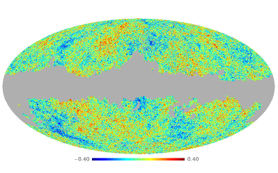
Figure 1 shows one of these simulated maps.

Figure 1: Example of one of our simulated lensed temperature map, using the procedure described in the text. Units are $mK_{\text{CMB}}$. The gray region corresponds to the Galactic mask we propose to use. A point-source mask is also included, but barely visible, being more clearly seen on Fig 5.

3 Update on the FS-inpainting method

In Perotto et al. (2010), we studied the impact of an inpainting method to fill in, with an appropriate statistical mixture, a rather small mask (cutting a $\simeq 10\%$ fraction of the sky). It was oriented toward component-separated maps, where such a level of final masking is to be expected. Here, we push the algorithm further to its limits by studying the filling of the large mask defined in Sect. 2 ($\simeq 30\%$ of the sky). Furthermore, we add spatially inhomogeneous noise, which most certainly affects the results of the algorithm.

Among the inpainting algorithm implemented within the Multi-Resolution on the Sphere (MRS) package, we found that the most robust results are obtained with the spherical harmonics $L_{1}$ norm minimization using wavelet packet variance regularization (Abrial et al. 2007, 2008).

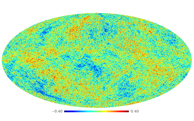
Each map from the $H_{0}$ and $H_{1}$ sets were inpainted. An example of a restored map is shown in Fig. 2.

Figure 2: Inpainted map corresponding to filling the Galactic+point-source mask of Fig 1.

We then apply the Hu&Okamoto quadratic estimator on the full-sky, using the fast spherical harmonic computations provided by the HealPix package, with a multipole cut $\ell_{\text{max}}=2000$, since there is no statistical gain in going to higher values given the noise level. The ”observed” temperature spectrum that enters the QE filter is estimated for each map, which is a way of ”absorbing” the residual spectrum deformation after the mask restoration. We did not adopt the Bielewicz’s trick and therefore insert the theoretical unlensed spectrum into the numerator of the QE filter. Given the resolution and noise, we also analytically computed the $N^{(1)}$ and $N^{(2)}$ terms using the fiducial lensing power spectrum.

The bias size can then be estimated in either the $H_{0}$ or $H_{1}$ simulations. In the former case, one directly measures a bias, after $N^{(0)}$ subtraction, that by construction, does not depend on the potential field. In the latter case, one can estimate the bias with respect to the fiducial model, after the $N^{(0)},N^{(1)}$, and $N^{(2)}$ corrections have been applied, that can grab some extra contributions. We wish to check the robustness of our correction of the lensing field, by estimating $N^{\text{MC}}$ i the $H_{0}$ set. The inpainting process is expected to induce a non-zero lensing coupled bias, since it cannot accurately restore the lensed signal statistic up to the four-point correlation function into the masked region. However, this effect can be effectively accounted for by introducing an $f_{\text{sky}}$factor to correct for the lack of power caused by the un-restored lensing modes within the mask, so that the QE variance is given by

$$\ell(\ell+1)\langle{\hat{\phi}_{\ell m}}^{*}{\hat{\phi}_{\ell^{\prime}m^{\prime}}}\rangle = \delta_{\ell\ell^{\prime}}\delta_{mm^{\prime}}(f_{\text{sky}}C_{\ell}^{\text{d}}+N_{\ell}^{dd}),$$

$$\text{where }N_{\ell}^{dd} = N_{\ell}^{(0)}+f_{\text{sky}}(N_{\ell}^{(1)}+N_{\ell}^{(2)})+N_{\ell}^{\text{MC}},$$ (8)

and the various contributions are shown in Fig. 3.

Figure 3: Mean deflection spectra reconstructed by applying the FS-inpainting method to the lensed maps. ”Raw lensing” denotes the spectrum reconstructed directly from the maps. In blue, we show the effect of correcting for the (known) analytical terms $N^{(1)}$ and $N^{(2)}$. In red, one subtracts the Monte Carlo correction obtained from the set of unlensed maps. The dashed line is the true input spectrum. All points are assigned an error bar corresponding to the sample variance of each map within our Monte Carlo set.

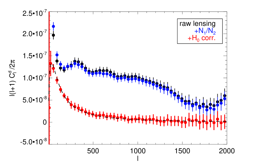
The bias of the estimator is quite important but corrected for by using the unlensed simulations. This means that the correction does not couple significantly to the lensing spectrum. It however still introduces systematic uncertainties related to our limited knowledge of the instrument. This motivates the development of an alternative method, which completely avoids the masking issue, to the detriment of introducing some new technicalities.

4 The local approach: multi-patch

We start with a simple question. How do you derive the power spectrum from a vector of sampled data? There are two approaches:

1. One solution is to perform a one step fast Fourier transform (FFT), which produces many modes that can then be averaged (binned) later on.

2. if the low frequency power spectrum is not required, a solution is to slice your sample into bunches, apodize each one, perform the individual FFTs, and take their mean.

Which approach is better? It was found that using the second one, with overlapping segments of data (by $\simeq 50\%$) provides the nicest (binned) estimates (Oppenheim & Schafer 1975). This is known as the Welsh periodogram. That then happens when some portion of the data is missing? In the first case, one tries to correct for the gaps, possibly by restoring a mixture that has the correct statistical properties given some prior of the signal, i.e. by performing an inpainting. It is much simpler in the multi-bunch case, where one rejects chunks that overlaps with the gaps, an approach that is efficient as long as there are few of them and they are largely contiguous.

In the following, we apply these ideas to the case of data located on a cut-sphere. We extend beyond the power spectrum estimation (which was largely studied in Das et al. (2009)) and investigate whether this simple idea can be applied to CMB lensing reconstruction, where the main ”gap” is the Galactic plane and the ”bunches” are some tangent square planes.

We thus developed a pipeline that allows for a local reconstruction of the CMB lensing in patches. This has the obvious advantage of avoiding the masked regions and should therefore not introduce the large bias due to the mask correlations that appears in a full-sky analysis. Furthermore, the noise inhomogeneity, which adds a sizable contribution to the lensing deflection, is also reduced by working locally.

Working spatially also allows us to easily inspect the quality of the data in different regions of the sky and therefore constrain the experimental systematics. The natural flat-sky formalism that is applied can be easily interpreted, and indicators, such as one for lensing isotropy, can be developed.

Statistically, after determining the Fourier complex coefficients for each patch, we use the Hu-Okamoto quadratic estimator (QE) described in Sect. 1. This has, by construction, a minimum variance so there is no statistical loss in using this approach. However, obviously, no scales below the patch Fourier size $\tfrac{2\pi}{L}$ can be reconstructed, hence we miss the low multipoles.

4.1 Tiling the cut-sphere with patches

The first unknown is the typical size ($L\times L$) of the patches that one must use for lensing. It turns out to be a compromise between several contradictory considerations:

1. Lensing correlates modes over a few degree scale.

2. The Fourier modes that are to be reconstructed are located at harmonics of $k_{0}=\tfrac{2\pi}{L}$ in each $(k_{x},k_{y})$ Fourier direction. For $L=5\degr,10\degr$ and $15\degr$, respectively, this corresponds to $k_{0}=72,36,24$, which sets the grid spacing of the measured modes. To derive our final result in reasonably small multipole bins, we therefore chose to adopt a large $L$ value.

3. When projecting the data from the sphere onto the local tangent plane (using a gnomonic projection), we wish to avoid too much distortion, which implies that we should not use too large $L$ values. The classical $L\lesssim 20\degr$ flat-sky upper limit to the flat sky approximation(White et al. 1999) was derived from power spectra considerations and is not necessarily valid for the four point statistics we consider in lensing.

4. A last consideration is the efficiency of tiling a given cut-sky surface with square patches, which causes them to be small. In addition, inspired by the Welsh periodogram, we seek a configuration where the patches overlap by about 50%, so that there is a clear interplay between the patch central positions and their sizes.

These considerations suggests that patches of angular size $\simeq 10\degr$ with $\simeq 50\%$ overlap are appropriate. Although it is a many-parameter system, we found that a simple solution is obtained with patches of angular size $L=10\degr$ located at the centers of a HealPix $n_{\text{side}}=8$ map pixels. In this case, each pixel in the sphere falls on average into $\simeq 1.8$ patches. We note that the tiling details do not impact the final result, since we performed the same analysis on $L=12\degr$ patches (which leads to a pixel on average falling into 2.6patches) and obtained very similar results.

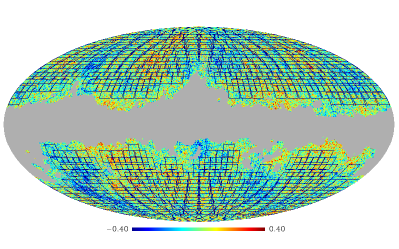
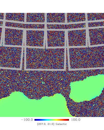
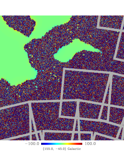
We then start with $12n_{\text{side}}^{2}=768$ patches. Only patches that do not intersect the Galactic mask at all (the reason being explained in the prewhitening section) are then kept, which leaves $395$ of them, covering a fraction $f_{\text{sky}}=55\%$ of the sky (as represented on Fig. 4). In this configuration, the overlap (the mean number of patches a point of the sphere belongs to) is $\simeq 1.7$.

Figure 4: Example of the tiling of the map shown on Fig. 1 with overlapping $10\degr\times 10\degr$ patches, that do not intersect the Galactic masked region.

4.2 Preparing the patches

Local point-source inpainting.

Before extracting the Fourier coefficients, we first need to remove the bright sources from the patches, which are a strong lensing contaminant. This is performed by using the point-source mask and filling the masked values by an inpainting algorithm. We note that we use an (image) inpainting algorithm that differs from the one described in Sect. 3, because we wish each patch to be treated independently of the others, which is not the case for FS-inpainting. We chose a method that has been designed and tuned for weak lensing surveys FastLens, which consists in minimizing the sparsity of DCT (discrete cosine transform) coefficients for $256\times 256$ data blocks.

More precisely, we construct high resolution regular images from the patches using bi-linear interpolation. The FastLens code is then run to fill in the point-source masked areas. The inpainted values are then back-projected onto the sphere to obtain again full-sky maps in which each sources belonging to a patch have been filled.

Since the patches overlap, some filled sources sometimes belong to several of them : we then use the inpainted values from the patch whose center is the closest to the source, in order to avoid border effects.

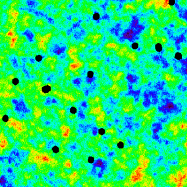
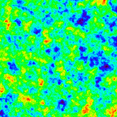
This procedure is applied to the full set of $H_{0}$ and $H_{1}$ simulations. An example is shown in Fig. 5

Figure 5: (a) Example of a $10\degr\times 10\degr$ patch with masked sources in black. (b) Inpainting of the sources using the FastLens algorithm.

Prewhitening and apodization.

At this stage, we could again project the pixels onto patches and reconstruct the Fourier coefficients (details in Sect. 4.3). However, we note that the bi-dimensional temperature power-spectra obtained for these patches exhibit a strong leakage along the null Fourier axis (Fig. 6(a) ).

Figure 6: (a) Bi-dimensional Fourier spectra of one of our simulation at different scales. Upper-left: mean of the squared-amplitude of the Fourier coefficients for all patches i.e. $k^{2}{\langle\lvert a_{{k_{x}},{k_{y}}}\rvert^{2}\rangle}$. An isotropic un-decimated wavelet transform (”a trous”, see e.g. Starck & Murtagh (2010)) is applied to the image and the results for scale one and two are shown in the bottom plots. The upper-right one corresponds to the smooth component. One notices a clear leakage along the null axes. (b) Same spectra but working on the prewhitened map and applying a Kaiser-Bessel $K_{0.5}$ window function. The leakage along the null axis has clearly disappeared.

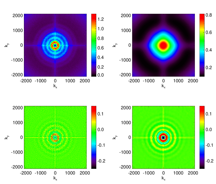
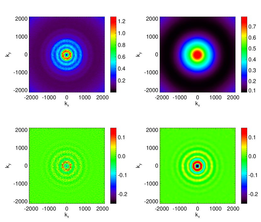
We concluded that this leakage is due to that of the low $(k_{x},k_{y})$ modes which, for the CMB signal, have the stronger amplitudes, and originates from the side-lobes of the implicit $10\degr\times 10\degr$ top-hat window used. Instead of using some anisotropic filtering (the lensing itself being a source of anisotropy), we can correct this by prewhitening the map and applying an explicit window.

Prewhitening is a standard means of achieving comparably sized Fourier coefficients (e.g. Das et al. 2009). Since we are interested in a range up to $\ell\simeq 2000$ (i.e. which is not too far into the CMB damping tail), we need to approximately scale the spectrum by $\ell^{2}$. We therefore simply multiply the spherical harmonic coefficients of the map by $\ell$, and return to direct space. In this process, the Galactic values are replaced by zero’s, which results in some ringing around the edges of the mask, which is fortunately damped by the instrument main lobe. This is why we only used patches that do not intersect the mask edges at all, since in practice, they are placed far enough away from the mask frontier. Two illustrative examples are shown in Figure 7.

Figure 7: Examples of the $10\degr\times 10\degr$ multi-patch tiling (in gray) of a prewhitened map, around the borders of the Galactic mask (in green) in two regions of the sky (Galactic coordinates given in degrees). One can discern some very local ringing around the boundaries of the mask and some point-sources located outside the patches and that had therefore not been previously inpainted.

We note that the prewhitening procedure was applied to both the ”signal” maps ($H_{1}$ set) and the MC-correction ones ($H_{0}$), so that if it still had a sizable impact on the lensing reconstruction it would have biased the final lensing estimate. Anticipating a result that is be presented later (Fig. 11), the $H_{0}$ correction is then found to be small, which validates a-posteriori the prewhitening procedure (and actually the entire procedure) is harmless to lensing.

From now on we work with these full-sky prewhitened maps for which the harmonic coefficients are of similar order.

Rather than using for each patch the implicit top-hat window (which has large side-lobes), we apply an explicit window in the direct space. We work with the family of Kaiser-Bessel functions (Kaiser 1966), which allow us to vary simply the side-to-main lobe ratio, and that is still close to the optimal solution of energy concentration provided by the discrete prolate spheroidal sequence (Slepian 1978; Das et al. 2009).

Each value in the $L\times L$ size patch is therefore multiplied by

$$W_{\alpha}(x,y) = W^{(1)}_{\alpha}(x)W^{(1)}_{\alpha}(y)$$ (9)

$$W^{(1)}_{\alpha}(x) = \dfrac{1}{I_{0}(\pi\alpha)}I_{0}\left(\pi\alpha\sqrt{1-\left(x/\tfrac{L}{2}\right)^{2}}\right),$$ (10)

where $I_{0}$ denotes the zero-th order modified Bessel function of the first kind.

The Fourier transform of these windows is

$$\tilde{W}_{\alpha}(k_{x},k_{y}) = \tilde{W}^{(1)}_{\alpha}(k_{x})\tilde{W}^{(1)}_{\alpha}(k_{y})$$

$$\tilde{W}^{(1)}_{\alpha}(k_{x}) = \dfrac{L}{I_{0}(\alpha\pi)}\sin_{\text{c}}\left(\sqrt{\left(\dfrac{k_{x}L}{2}\right)^{2}-(\alpha\pi)^{2}}\right),$$ (11)

which exhibits how the windows shrinks with $\alpha$ when comparing it to the tophat window in Fourier space: $\tilde{W}^{(1)}(k_{x})=\sin_{\text{c}}(\tfrac{k_{x}L}{2})$.

We compute numerically the radial power of these windows as :

$$P_{W}(r) = \dfrac{1}{2\pi}\int_{0}^{2\pi}|W_{\alpha}(r\cos\phi,r\sin\phi)|^{2}d\phi$$

$$P_{\tilde{W}}(k) = \dfrac{1}{2\pi}\int_{0}^{2\pi}|\tilde{W}_{\alpha}(k\cos\theta,k\sin\theta)|^{2}d\theta$$ (12)

and show them for $\alpha=0.5,1,2$ on Fig. 8 in direct and Fourier space.

Figure 8: Radial power of the Kaiser-Bessel 2D windows with $\alpha=0.5,1,2$ for $L=10\degr$ in real (a) and Fourier (b) space. The top-hat result is also shown.

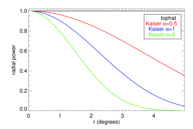
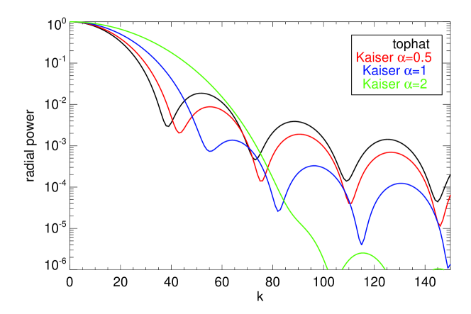
As is well-known, diminishing the side-lobes always occurs at the price of increasing the main lobe width (energy conservation). In the following, we describe how we attempted to keep $\alpha$ as small as possible to keep the window strongly peaked since the QE considers the products of modes are convolved by this window in Fourier space (Sect. 4.5).

We checked that after prewhitening and windowing with the Kaiser($\alpha=0.5$) window, the power spectrum leakage disappears as is clear on Fig. 6(b). In the following, we therefore use $W_{0.5}$ as an explicit apodization function.

The size of the window in Fourier space , Fig. 8(b), fixes the binning. For $W_{0.5}$ on a $L=10\degr$ square patch, we use a step of $\Delta k=40$, starting from the first available Fourier mode $k_{0}=35$,

4.3 Fourier series estimation of non-equispaced data

We project the prewhitened map onto the local patches, using a gnomonic projection. The HealPix pixel centers then fall onto an irregular bi-dimensional grid. Can we still perform a spectral analysis ?

For a $n_{\text{side}}=2048$ HealPix map, the mean inter-pixel separation is about $1.7\arcmin$, which is not negligible compared to the expected mean deflection of the CMB lensing ($\simeq 2.7\arcmin$), so that an interpolation would induce some large effects. To avoid this interpolation, we therefore developed the so-called ”ACT” (Adaptive weight, Conjugate gradient, Toeplitz matrices) algorithm, which allows us to fit the complex Fourier coefficients from a set of irregularly sampled data in a reasonable time (see also Keiner et al. (2009)). This method has been proposed for real (1D) data and we generalized it to bi-dimensional data. We give hereafter the main idea and discuss the technicalities in the Appendix.

We search for the least squares estimates of the $a_{k,h}$ (complex) Fourier coefficients of our band-limited temperature signal, in the series expansion

$$T(x,y)=\sum_{k=-M_{x}}^{M_{x}}\sum_{h=-M_{y}}^{M_{y}}a_{k,h}e^{2i\pi k\frac{x}{L}}e^{2i\pi h\frac{y}{L}}.$$ (13)

In the general case, the brute force inversion of the normal equations is prohibitive, but the method takes advantage of the peculiar structure of the Fourier series decomposition to perform operations very efficiently. In our case, we manage to determine the $120\times 120$ coefficients of the $\simeq 120\leavevmode\nobreak\ 000$ data values contained in a $10\degr\times 10\degr$ patch of an HealPix $n_{\text{side}}=2048$ map, in about one minute on a single core computer.

The tool we developed, named FourierToeplitz, has been compared to a standard FFT method, when fitting (actually solving) $N\times N$ points with $N\times N$ unknowns on a regular grid: our results agree to within machine precision.

This tool opens the road to local analyses of projected spherical maps, which are plagued by interpolation issues. It has been used successfully in computing the spectra and full CMB bi-spectra in Pires et al. (2012).

4.4 Local power spectra estimates

After running the FourierToeplitz tool, we have an estimate of the complex Fourier coefficients per patch, at wave-vector $\@vec{k}$, located on the regular grid Eq. (7).

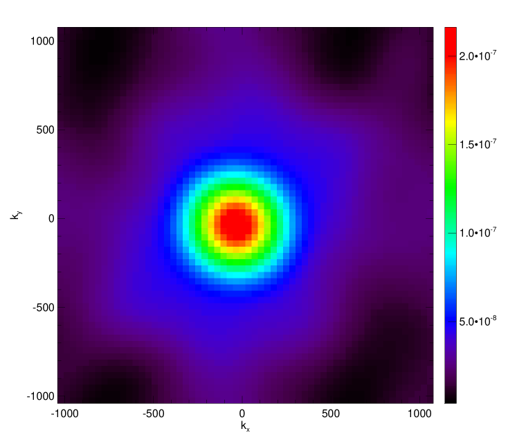
By computing the squared-amplitude map, one can study the 2D local power spectrum on the sky, and even though the cosmic variance is large, detect potential experimental problems. By taking the mean of the power spectra for all the patches, one can check for the CMB field isotropy in a simple way.

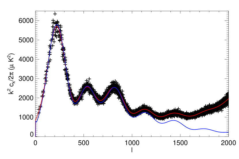
By plotting the values, with respect to $\lvert\@vec{k}\rvert$ (i.e. assuming isotropy), one constructs a 1D power spectrum which is equivalent to the famous $C_{\ell}$ but for the non-integer values $\lvert\@vec{k}\rvert$ given by Eq. (7). One has a powerful local power-spectrum estimator that solves the issues of masking that is well-suited to jackknife tests. To get a full determination of the spectrum, one would still have to study the window function, as in Hivon et al. (2002) and Das et al. (2009), but we do not actually need it for the lensing reconstruction since it relies on the observed spectrum. We first need to deconvolve the maps from the main lobe, which is a trivial operation in the Fourier space for a Gaussian shape, and obtain some smooth spectrum. This is obtained by taking the mean power spectrum of the de-convolved Fourier patches, and fitting the coefficients of a generic smooth function to all the data points as explained in Plaszczynski & Couchot (2003). The result is shown for one of our simulation, in Fig. 9.

Figure 9: Example of a 1D power spectrum used in the lensing estimator. The points are obtained from the bi-dimensional spectrum (as in Fig. 6(b)), deconvolved from the beam, and represented with respect to to $\lvert\@vec{k}\rvert$. They are fitted to the smooth function in red. Also shown in blue is the fiducial model.

4.5 Local deflection estimates

After determining the complex Fourier coefficients for each patch, and the observed/true $C_{\ell}$’s, we may apply the Hu&Okamoto flat-sky estimator to obtain the (noisy) potential maps in the Fourier domain, Eq. (2). But before going on to the lensing spectrum estimate, we need to review the noise of the estimator on an apodized patch since the standard QE has not been derived in this case.

The quadratic term $\langle T(\@vec{k}_{1})T(\@vec{K}-\@vec{k}_{1})\rangle$ upon which the estimator in Eq. (2) is build, is affected in a non-trivial way by the apodization procedure. Metcalf & White (2007, Appendix B) show that it introduces:

1. An ”aliasing” effect due to the overlap of the windows in Fourier space that affects only the low $\ell$’s modes.

2. Some complicated ”smoothing” of the lensing potential.

We do not try to build an optimal estimator from the elaborate expression. We note instead that the apodization process scales the lensing Gaussian noise merely by a constant factor, that can be understood in the following way.

On the basis of Hivon et al. (2002) and Efstathiou (2004), one can show that, assuming that the window is well peaked in Fourier space such that the spectrum does not vary too much over it, the two-point correlation function of an apodized Gaussian field $T^{\textrm{apo}}$ along with its variance can be approximated by

$${\langle T^{\textrm{apo}}(\@vec{k}_{1})T^{\textrm{apo}}(\@vec{k}_{2})\rangle} \simeq (2\pi)^{2}\delta(\@vec{k}_{1}+\@vec{k}_{2})w_{2}C_{k_{1}}$$ (14)

$$\textrm{var}(T^{\textrm{apo}}(\@vec{k}_{1})T^{\textrm{apo}}(\@vec{k}_{2})) \simeq 2w_{4}C_{k_{1}}C_{k_{2}},$$ (15)

where

$$w_{i}=\dfrac{1}{L^{2}}\int_{-L/2}^{L/2}\int_{L/2}^{L/2}dxdyW^{i}(x,y)$$ (16)

and $W(x,y)$ is the window function in direct space.

These approximations are accurate for large $k$ values (Efstathiou 2004), which corresponds, given our window size to $k\gtrsim 100$.

In the following, we use windows normalized by $\sqrt{w_{2}}$, so that the reconstructed power spectrum, the only entity that varies with apodization in the filter/normalization of the QE, Eq. (1), is mainly unchanged (Eq. (14)). We checked for instance that applying a $W_{0.5}$ window would change the lensing normalization $A_{k}$ by less than 1%.

The Gaussian noise in the apodized case can be written as the variance in the QE applied to the apodized unlensed sky:

$$N_{K}^{(0,\textrm{apo})}=K^{2}{\langle\lvert\hat{\phi}^{\textrm{unlens, apo}}(\@vec{K})\rvert^{2}\rangle}.$$ (17)

Substituting Eq. (15) into this equation and using the normalized window, one obtains

$$N_{K}^{(0,\textrm{apo})}\simeq\frac{w_{4}}{(w_{2})^{2}}N_{K}^{(0)}.$$ (18)

What is the accuracy of this approximation? We ran the QE on the unlensed simulations, computed the mean lensing spectrum and compared it to the ideal case given by Eq. (5). The result in Fig. 10 shows that the ratio is indeed reasonably flat for values of $\ell\gtrsim 100$. Fitting the mean value of this ratio in the high $\ell$ region gives a result very close to the analytical value $\tfrac{(w_{2})^{2}}{w_{4}}=0.859$.

Figure 10: Color plots showing the ratio of the non-apodized $N^{(0)}$ term Eq. (5) to the reconstructed lensing variance in the patches apodized by $W_{0.5}$ for each of the 100 maps of our unlensed ($H_{0}$) set. A constant term, whose value is depicted in the upper box, is fitted to the $\ell\geq 1000$ part.

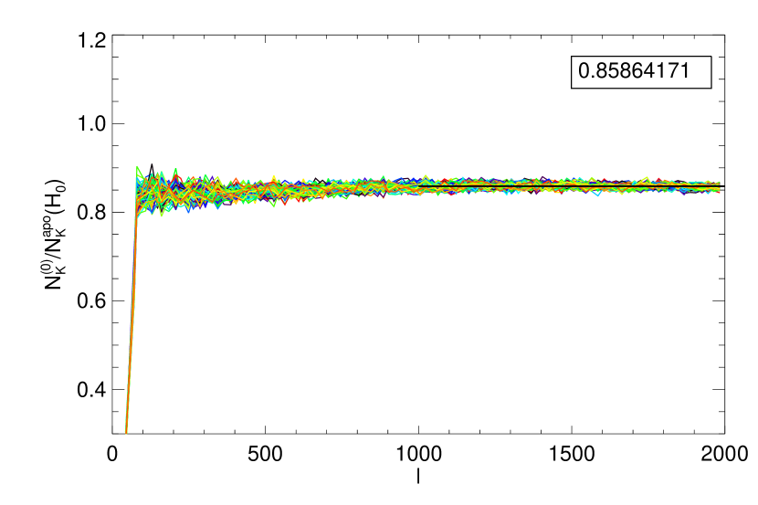
We performed the exercise for several windows, including the often used Hanning one (e.g. Oppenheim & Schafer 1975), and give our results in Table 1) . They all show excellent agreement with the simple $\tfrac{(w_{2})^{2}}{w_{4}}$ scaling factor.

window	$\tfrac{(w_{2})^{2}}{w_{4}}$	MC-$H_{0}$
Top-hat	1	1
Kaiser($\alpha=0.5$)	0.859	0.859
Kaiser($\alpha=1$)	0.502	0.505
Kaiser($\alpha=2$)	0.248	0.249
Hanning	0.264	0.265

Table 1: Comparison of the lensing excess Gaussian noise due to various apodization windows. $\tfrac{(w_{2})^{2}}{w_{4}}$ is the analytical approximation, whereas the last column gives the measured ratio from the unlensed Monte Carlo’s, obtained as on Fig. 10.

This leads us to rewrite the QE total covariance Eq. (6) in the apodized case, as

$$\begin{split}K^{2}{\langle{\hat{\phi}(\@vec{K})}^{*}{\hat{\phi}(\@vec{K}^{\prime})}\rangle}&=(2\pi)^{2}\delta(\@vec{K}-\@vec{K}^{\prime})\\ &\cdot\dfrac{w_{4}}{(w_{2})^{2}}[C_{K}^{d}+N_{K}^{(0)}+N_{K}^{(1)}+N_{K}^{(2)}+N_{K}^{\text{MC}}]\end{split}$$ (19)

and propose the simple estimator for an apodized patch

$$K^{2}\widehat{C_{K}^{\phi}}=\frac{(w_{2})^{2}}{w_{4}}\int\frac{d\phi}{2\pi}K^{2}|\hat{\phi}^{\textrm{apo}}(\@vec{K})|^{2}-(N_{K}^{(0)}+N_{K}^{(1)}+\cdots)$$ (20)

where the integral is performed in small size rings over the discrete Fourier grid.

This proposed estimator, Eq. (20), is then tested on our $H_{1}$ simulations in order to assess its bias/variance. We note that the value of the scale factor does not need to be known very precisely. What matters is that the same factor is used in the data (here $H_{1}$) and the Monte Carlo correction (here $H_{0}$).

We now have all in hand to compute the deflection power-spectra. This is performed for each map of our Monte Carlo set, in the following way:

1. From the Fourier coefficients obtained on each patch, we form the 2D-Fourier potential map $\hat{\phi}$ using Eq. (2). The normalization (and $N^{(0)}$ term) is computed in the standard way, using Eqs. (5) and (1) and the true/observed spectrum as given in Fig. 9.

2. For each patch, we form the noise-corrected deflection power map of $fK^{2}\lvert\hat{\phi}_{K}\rvert^{2}-N_{K}^{(0)}$ where $f=0.86$ in our case.

3. We accumulate the 395 power maps and evaluate their mean and variance.

4. We compute the inverse-variance weighted average in rings of constant $\Delta K=40$ width (starting at $K_{0}=35$). The binned values are reported at the mean of the different modes $K_{i,j}$ locations within the ring.

We compute these spectra in the $H_{1}$ set, which still have noise contributions from the $N^{(1)}$, $N^{(2)}$ and $N^{\text{MC}}$ terms. The $N^{\text{MC}}$ term (the ”bias”) is taken from the $H_{0}$ simulations as the mean difference from 0 of the reconstructed spectra following the same procedure.

The mean spectrum is shown in Fig. 11, where one sees the various contributions.

Figure 11: Mean deflection spectra reconstructed by the multi-patch method from the lensed maps. ”Raw lensing” denotes the spectrum measured directly on the maps as described in the text without performing any bias correction. In blue, we show the effect of subtracting the (known) analytical terms $N^{(1)}$ and $N^{(2)}$. In red, one accounts for the Monte Carlo correction obtained for the set of all unlensed maps. The dashed line is the fiducial input spectrum. All points are assigned an error bar corresponding to the variance in the Monte Carlo simulations per sky map. The first bin for the raw-lensing estimate is located outside the plot (at a value of $3.5\times 10^{-7}$). The same range as on Fig. 3 has been used for proper comparison.

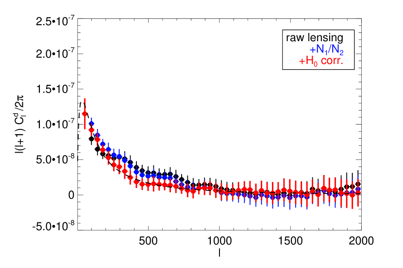
The initial (raw) lensing spectrum estimate already has a very little bias, thanks to our lack of use of any Galactic data and to a reduced local noise inhomogeneity.

We show that the multi-patch method leads, after a small correction, to an un-biased estimate of the deflection over the whole $\ell\in[75,2000]$ range. The very first bin $[35,75]$ is also unbiased but receives a stronger correction from the $H_{0}$ MC, which is due to the breakdown of the flat-sky limit ($\ell$ cannot be identified to $\lvert\@vec{k}\rvert$ in this case) and to the apodization window having an overlap integral that extends to approximately 100 (see Fig. 8(b)).

We note that unlensed simulations accurately correcting the lensed ones means that the full reconstruction process does not induce any (significant) couplings to the underlying lensing potential. The variance in the estimator is discussed in the next part.

Finally, we note that working on patches has a number of other benefits:

1. We derive bi-dimensional maps of the lensing potential, so that as in Fig. 6, we can more easily test the deflection field isotropy. An example is show in Fig. 12.

2. For each patch, we can check for unexpected systematic error effects that would provide an excessive lensing signal (as missed sources).

3. With knowledge of all sources of noise, one can apply a Wiener filter to each patch to reconstruct the lensing potential maps that can then be cross-correlated to other cosmological probes of the matter, such as Galactic weak lensing (cosmic Shear) or cosmic infrared background, which are only generally measured over a small region of the sky.

Figure 12: Example of an isotropy check of the lensing potential. For one of our lensed maps, we evaluate the ”raw lensing” estimator (i.e. that does not include any MC correction) for each patch, and take their mean. We represent the power map $k^{4}\hat{C}_{k}^{\phi}$ after $N^{(0)}$ subtraction, and smoothed by an ”a trous” transform, as in the upper right part of Fig. 6(b).

5 Comparison of the methods

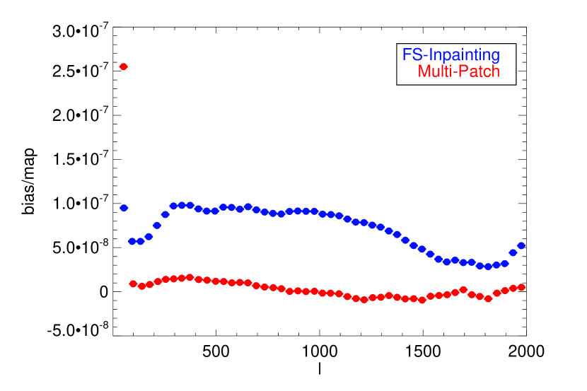
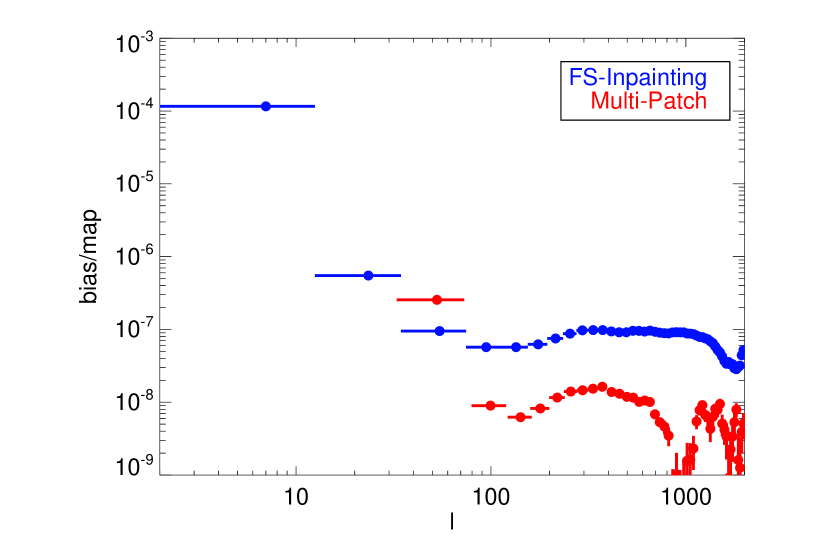
In Fig. 13, we compare the bias, in each $\ell$ bin, of the FS-inpainting and multi-patch methods. They were obtained using unlensed simulations, and were indeed shown to correct the deflection power measure in lensed maps. We recall that the binning that we used starts at $\ell=35$ (first multi-patch accessible mode for a $10\degr\times 10\degr$ patches) and has a width $\Delta\ell=40$. Two extra bins were added to FS-inpainting $[2,13]$ and $[14,34]$.

Figure 13: (a) Bias of the methods computed from our simulations as the mean of the spurious deflection power on the unlensed set. For FS-inpainting, it corresponds to $N_{\ell}^{\text{MC}}/f_{\text{sky}}$ in Eq. (3), whereas for multi-patch, it is the result of applying the modified QE to $H_{0}$ as described in Sect. 4.5. (b) Same plot with a log scale to emphasize the low $\ell$’s. No mode below 35 is available to the multi-patch method.

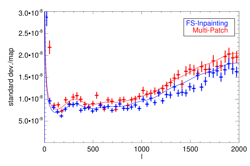
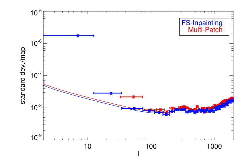
The standard deviation in each bin from the $H_{1}$ set is shown in Fig. 14. The Fisher error estimate for the QE

$$\sigma_{\ell}=\dfrac{C_{\ell}^{\text{d}}+N_{\ell}^{(0)}}{\sqrt{\ell\Delta\ell f_{\text{sky}}}}$$ (21)

is also depicted. We recall that the multi-patch method has a lower sky coverage ($f_{\text{sky}}=0.55$ ) than the inpainted one ($f_{\text{sky}}=0.69$ ) owing to the procedure for tiling the cut-sky.

Figure 14: (a) Standard deviation among the methods computed from our simulations, as the spread in each bin of the lensing estimators for the 100 $H_{1}$ set. (b) Same plot with a log scale to emphasize low $\ell$’s.

From these plots, it appears that

• The multi-patch approach clearly shows less bias, except for the very first bin $[35,75]$. It cannot reconstruct modes below these values.

• For large $\ell\gtrsim 100$, both estimators follow the naive Fisher error estimates, the FS-inpainting one having a slightly smaller variance than for multi-patch, owing to the larger sky coverage.

We feel that the small relative statistical loss ($\simeq 10\%$) of the multi-patch method is largely compensated for by the gain on systematic errors. As explained in Sect. 4, the reconstruction can be controlled and visually inspected at each step, but most importantly the systematic errors due to the bias of a necessarily imperfect simulation are minimized.

We therefore advocate the use of an hybrid method consisting in the multi-patch approach for $\ell\gtrsim 100$ and FS-inpainting for lower $\ell$’s.

Conclusion

We have investigated two methods to reconstruct the lensing-deflection power spectrum from PLANCK-like CMB frequency maps, using a large Galactic cut and including some strong noise inhomogeneity. The first one, FS-inpainting, which was previously presented in Perotto et al. (2010), is still found to be efficient in this extreme configuration as long as one corrects for a large yet lensing-independent bias using Monte Carlo simulations. We have developed a well-suited method to deal with large masks, based on tiling the cut-sky with $10\degr\times 10\degr$ patches and performing local analyses. This has required us to solve some problems related to non-periodic boundary conditions and Fourier coefficients determination for irregularly sampled 2D data. For this purpose, we have developed the FourierToeplitz tool, which allows the fast exact fitting of the Fourier series coefficients in irregularly sampled 2D data. This is a valuable tool for other analyses that require a high level of precision at the spatial location.

Both methods have been demonstrated for realistic PLANCK-like simulations of the 217 GHz CMB channel. It was found that the multi-patch approach has a very low bias in the whole $100\leq\ell\leq 2000$ range, thanks to the avoidance of the Galactic plane, and lower local noise inhomogeneity. It allows us at each step to check for experimental systematic errors and perform local images of both the temperature and deflection bi-dimensional power spectra. Its final variance is only marginally larger than a full-sky method, and could be improved by a smarter strategy for tiling the cut-sky sphere. The final result is insensitive to the precise position of the patches and of their overlap. To perform some cosmological fits using the reconstructed spectrum, the inter-bin correlation would still have to be measured accurately, and included in the likelihood, since we have measured some $(15\pm 10)\%$ correlation level, with our $\Delta\ell=40$ binning. This requires a large number of simulations ($\simeq 1000$).

In the $\ell\leq 100$ range, we advocated using the FS-inpainting method, which provides the minimal variance estimate in the cut sky. Since our simulations did not include a Galactic contaminant, this boundary could slightly shift. However, using our $30\%$ Galactic mask, we checked by adding a simulated Galactic component to our maps, that its net effect on the reconstructed deflection power was extremely negligible (on real data, some template would be subtracted).

These results open the road to measuring CMB lensing directly in PLANCK-like CMB maps, without even performing a component separation of the foregrounds. This is not exactly true for the FS-inpainting method, where one must have clean boundaries at the mask frontier. However, this can be obtained by a simple template subtraction measured in the high frequency channels. For the multi-patch method, one can still perform the analysis without ”un-dusting” the map, by choosing appropriate CMB-dominated patches; we checked in simulations that a sub-dominant amount of dust contamination does not affect the lensing deflection spectrum.

It is not our goal to come to a decision on whether a component separation method is a more accurate means of lensing reconstruction, since it is an area that remains under active development. We note however that the statistical gain offered by using a larger fraction of the sky can be counterbalanced by a higher $N^{(0)}$ term due to a larger (combined) lobe of the instrument or a higher final noise level (see Eq. (21)). Adding the high/low frequency channels will also ”bring back” some additional infrared/radio sources that need to be masked out, lowering the final statistical gain of the combined map.

Working directly on intensity maps allows us to perform various sanity tests by checking the consistency between the reconstructions from different frequency maps, which is a way of assessing the robustness of the estimate against either experimental uncertainties or physical contamination – as from possible SZ-lensing or unresolved radio-source-lensing correlations. The reconstructions of each frequency maps can also be minimum-variance combined, which offers a robust reconstruction that allows for a high level of systematic control. Finally, this is a well-suited approach to cross-correlation studies with other mass tracers, by selecting frequencies that are unaffected by contaminants that may induce extra correlations. For instance, one may wish to use only frequencies over 100 GHz (with negligible unresolved radio-source contamination), while studying correlations with external radio surveys, or below 217GHz for a CIB-lensing correlation estimate.

Appendix: FourierToeplitz tool

In order to not lose accuracy in determining the Fourier coefficients from a sample of irregularly sampled points, we developed a tool for fitting these coefficients in a reasonable time.

We start with the 1D case, where we have implemented the ”second generation” algorithm proposed in Feichtinger et al. (1995).

We define $f$ to be a function sampled on any support $\{t_{i}\}$. In a given interval $(0,T)$, the function can be expanded into a Fourier series

$$f(t)=\sum_{k=-\infty}^{\infty}a_{k}e^{2i\pi k\frac{t}{T}}.$$

Assuming that it has a band-limited spectrum, so that we can limit the number of Fourier modes to

$$f(t)=\sum_{k=-M}^{M}a_{k}e^{2i\pi k\frac{t}{T}},$$

the problem is to determine the $a_{k}$ coefficients given the sampled values $f_{i}$.

We consider the reduced $u=\tfrac{t}{T}$ variable. If the number of samples $u_{i}$ is N, one writes the N equations

$$f_{i}=\sum_{k=-M}^{M}a_{k}e^{2i\pi ku_{i}}.$$

This is a linear system of N equations with 2M+1 unknowns. The well- known normal equations obtained from least squares minimization are

$$(G^{T}G)X=G^{T}F,$$

where $F$ is the column vector of sampled values and $G$ is the matrix with elements $g_{kl}=e^{2i\pi ku_{l}}$. The solution is in general computationally heavy using standard methods.

Here, the interesting point is that the generic term of the system is of the type:

$$T_{kl}=\sum_{j=1}^{N}e^{-2i\pi(k-l)u_{j}},$$

which is a Toeplitz matrix. One solves the system using the conjugate-gradient algorithm (the matrix is Hermitian and positive), which consists in performing successive matrix-vector products. One then pads the Toeplitz matrix with zeros to obtain a circulant matrix, since the product of a circulant matrix with a vector can be computed efficiently using an FFT.

We extended this method to the 2D case using the formalism of the Kronecker products of matrices and the properties of the separability of FFTs. This allows for the fast determination of the $a_{kh}$ coefficients in the Fourier expansion

$$f(x,y)=\sum_{k=-M_{x}}^{M_{x}}\sum_{h=-M_{y}}^{M_{y}}a_{kh}e^{2i\pi k\frac{x}{T_{x}}}e^{2i\pi k\frac{ty}{T_{y}}}.$$

In our case, a $10\times 10\degr$ patch from an HealPix $n_{\text{side}}=2048$ map, contains about $120000$ irregularly sampled values.

The modes are harmonics of $\Delta k_{x}=\Delta k_{y}=\tfrac{2\pi}{L}\simeq 35$, so we need to determine $120\times 120$ (half is negative) of them to obtain all modes below $l_{max}=2000$. This is performed in about one minute on a single core. The conjugate gradient converges in about seven iterations, without using any special pre-conditioner, so we did not add the adaptive weight scheme.

References

- Abrial et al. (2007) Abrial, P., Moudden, Y., Starck, J., et al. 2007, Journal of Fourier Analysis and Applications, 13, 729
- Abrial et al. (2008) Abrial, P., Moudden, Y., Starck, J.-L., et al. 2008, Statistical Methodology, 5, 289, arXiv:0804.1295
- Ade et al. (2011a) Ade, P. A. R., Aghanim, N., Arnaud, M., et al. 2011a, A&A, 536, A8
- Ade et al. (2011b) Ade, P. A. R., Aghanim, N., Arnaud, M., et al. 2011b, A&A, 536, A7
- Ade et al. (2011c) Ade, P. A. R., Aghanim, N., Arnaud, M., et al. 2011c, A&A, 536, A23
- Beichman et al. (1988) Beichman, C. A., Neugebauer, G., Habing, H. J., Clegg, P. E., & Chester, T. J., eds. 1988, Infrared astronomical satellite (IRAS) catalogs and atlases. Volume 1: Explanatory supplement, Vol. 1
- Challinor & Lewis (2005) Challinor, A. & Lewis, A. 2005, Phys. Rev. D, 71, 103010
- Das et al. (2009) Das, S., Hajian, A., & Spergel, D. N. 2009, Phys. Rev. D, 79, 083008
- Das et al. (2011) Das, S., Sherwin, B. D., Aguirre, P., et al. 2011, Physical Review Letters, 107, 021301
- Efstathiou (2004) Efstathiou, G. 2004, MNRAS, 349, 603
- Feichtinger et al. (1995) Feichtinger, H., Groechenig, K., & Strohmer, T. 1995, Numer. Math., 69, 423
- Gold et al. (2011) Gold, B., Odegard, N., Weiland, J. L., et al. 2011, ApJS, 192, 15
- Górski et al. (2005) Górski, K. M., Hivon, E., Banday, A. J., et al. 2005, ApJ, 622, 759
- Hanson et al. (2010) Hanson, D., Challinor, A., Efstathiou, G., & Bielewicz, P. 2010, ArXiv e-prints
- Hanson et al. (2009) Hanson, D., Rocha, G., & Górski, K. 2009, MNRAS, 400, 2169
- Hirata & Seljak (2003) Hirata, C. M. & Seljak, U. 2003, Phys. Rev. D, 67, 043001
- Hivon et al. (2002) Hivon, E., Górski, K. M., Netterfield, C. B., et al. 2002, ApJ, 567, 2
- Hu (2000) Hu, W. 2000, Phys. Rev. D, 62, 043007
- Hu & Okamoto (2002) Hu, W. & Okamoto, T. 2002, ApJ, 574, 566
- Jarrett et al. (2001) Jarrett, T. H., Van Dyk, S., & Chester, T. J. 2001, in Bulletin of the American Astronomical Society, Vol. 33, American Astronomical Society Meeting Abstracts #198, 856
- Kaiser (1966) Kaiser, J. F. 1966, In Kuo, F. F. and Kaiser, J. F. (Eds.), System Analysis by Digital Computer, chap. 7 (New York, Wiley)
- Keiner et al. (2009) Keiner, J., Kunis, S., & Potts, D. 2009, ACM Trans. Math. Software., 36,4
- Kesden et al. (2003) Kesden, M., Cooray, A., & Kamionkowski, M. 2003, Phys. Rev. D, 67, 123507
- Larson et al. (2011) Larson, D., Dunkley, J., Hinshaw, G., et al. 2011, ApJS, 192, 16
- Lesgourgues & Pastor (2006) Lesgourgues, J. & Pastor, S. 2006, Phys. Rep., 429, 307
- Lewis & Challinor (2006) Lewis, A. & Challinor, A. 2006, Phys. Rep., 429, 1
- Lewis et al. (2000) Lewis, A., Challinor, A., & Lasenby, A. 2000, ApJ, 538, 473
- Metcalf & White (2007) Metcalf, R. B. & White, S. D. M. 2007, MNRAS, 381, 447
- Okamoto & Hu (2003) Okamoto, T. & Hu, W. 2003, Phys. Rev. D, 67, 083002
- Oppenheim & Schafer (1975) Oppenheim, A. V. & Schafer, R. W. 1975, Digital Signal Processing (Upper Saddle River, NJ, USA: Prentice Hall Press)
- Perotto et al. (2010) Perotto, L., Bobin, J., Plaszczynski, S., Starck, J.-L., & Lavabre, A. 2010, A&A, 519, A4
- Perotto et al. (2006) Perotto, L., Lesgourgues, J., Hannestad, S., Tu, H., & Y Y Wong, Y. 2006, J. Cosmology Astropart. Phys, 10, 13
- Pires et al. (2012) Pires, S., Plaszczynski, S., & Lavabre, A. 2012, Statistical Methodology, 9, 71 , special Issue on Astrostatistics + Special Issue on Spatial Statistics
- Pires et al. (2009) Pires, S., Starck, J.-L., Amara, A., et al. 2009, MNRAS, 395, 1265
- Planck Coll. (2005) Planck Coll. 2005, Blue Book (ESA), available from http://www.rssd.esa.int/planck
- Planck HFI Core Team et al. (2011) Planck HFI Core Team, Ade, P. A. R., Aghanim, N., et al. 2011, A&A, 536, A6
- Plaszczynski & Couchot (2003) Plaszczynski, S. & Couchot, F. 2003, ArXiv Astrophysics e-prints
- Slepian (1978) Slepian, D. 1978, The Bell System Technical Journal, 57, 5, 1371
- Smith et al. (2007) Smith, K. M., Zahn, O., & Doré, O. 2007, Phys. Rev. D, 76, 043510
- Smith et al. (2003) Smith, R. E., Peacock, J. A., Jenkins, A., et al. 2003, MNRAS, 341, 1311
- Starck et al. (2006) Starck, J.-L., Moudden, Y., Abrial, P., & Nguyen, M. 2006, A&A, 446, 1191
- Starck & Murtagh (2010) Starck, J.-L. & Murtagh, F. 2010, Astronomical Image and Data Analysis (Springer)
- Stompor & Efstathiou (1999) Stompor, R. & Efstathiou, G. 1999, MNRAS, 302, 735
- van Engelen et al. (2012) van Engelen, A., Keisler, R., Zahn, O., et al. 2012, ArXiv e-prints
- White et al. (1999) White, M., Carlstrom, J. E., Dragovan, M., & Holzapfel, W. L. 1999, ApJ, 514, 12