Nodal domain partition and the number of communities in networks

1 Introduction

With the surveys of many real-world networks, including the World-Wide Web [2, 22], metabolic networks [29, 23], epidemiology [36, 43], scientific collaborations and citation networks [38, 45], plenty of models were proposed to study their topological features and dynamic behaviors, such as the WS model [13], BA model [1] and Random Configuration model [10]. Recently, a particular and useful network structure, which is called “communities or clusters”, has been appealed to considerable attention. For its having no precise definition yet, common description about communities is division of nodes into groups with dense connection inside and sparse connection outside, by which mean communities could play an important role as the basic functional components in the foundation of complex networks.

Practically, part of scientists concern with nodes’ or edges’ individual behaviors affecting the surroundings [24, 19], while some others focus on the dynamics of ensembles of all the nodes in networks [3, 14]. These two special emphasis clarifies two possible directions in community detection: (1)detail exploitation: identifying nodes or edges whose absence influences networks’ dynamic most, which mostly are the boundary parts; (2)global sights testing for partitions structure either close enough to the original network or distinct most from the corresponding random pattern network.

It has been long accepted that centrality measures [46, 20, 21, 31] works well in characterizing relative importance of a node in a network [4, 46, 25], as well as similar scales on edges. In 2002, a fast algorithm aiming at identifying each edge of the network a betweenness measure gave rise to a explosive growth of activities in this field. Girvan and Newman [27] used the scale to quantify edges’ roles in the information transmission following paths of minimal length across the network. Removal of edges with high betweenness could lead to an exposure of the community structure.

Besides these detail exploitation methods, scientists also take the network whole into account, at which point two extreme situations might be queried: how much the original network shifts from its corresponding un-clustered version and spontaneously the well-clustered one.

Consideration on the first situation educed one of the most popular quality functions, so called modularity [39, 41, 42]. The basic thought was to compare the difference between total actual fractions of edges inside groups and the expected fractions when edges were placed at random. An improved version [41] was also developed to measure the difference between actual network and null model which yielded networks that were not supposed to have natural community structures [37, 41].

Furthermore, a probabilistic framework embedded with ‘stochastic matrices’ provides another important quality function [16, 17]. By introducing a metric on the space of Markov chains $K$ which represent random walks on the network [17], simple stochastic structure could be finally detected as the best approximation to the dynamics behaviors of $K$. This simple structure may contain the community information of the original network.

Despite the algorithm complexity of NP-hard [34], improved approximation techniques in partition problems calculate ‘optimized’ partition under certain constraints [40, 41, 28, 16], however, the question about the number of communities is still not easy to be answered [41, 17].

In this paper we introduce a method applying weak-nodal-domain partition(WNDP) which can suggest the number of clusters by exploring the information in the Laplacian eigenvectors. In Sec.II, we begin with a brief review of the spectral partition method and classical Nodal domain Theorem. In Sec.III, the main method and algorithm will be presented respectively. In Sec.IV, the algorithm is applied to three real network cases with fast and efficient results. In Sec.V, exceptional case is demonstrated for the further understanding of the method.

2 Spectral Partition and Nodal Domains Theory

The exactly mathematical definition of cluster has not been explicit so far, as though common agreement is focused on the minimization of edges whose disappearance will separate the network into groups with no inter-connection. A reasonable mathematical framework should be required to grasp the essential properties of the network not only precisely but also effectively. Particularly, quite a number of the clustering methods are involved with special matrices, for example, adjacency matrix, Graph Laplacian et al. All these matrices share the topological information of the networks ostensibly or inconspicuously.

So far, surprising results have already been made clear that eigenvectors of special matrices do work well in clustering [11, 35]. Scientists are interested in the projection from properties of these matrices to the corresponding networks’ outperforming structure. In the following sections, the eigenvectors of the Graph Laplacian $\mathcal{L}$ will be served as a tool to detect and analyze the community structure of the networks.

2.1 Spectral Partition

Let $G=(V,E)$ be an undirected graph with labeled vertex set $V=\{1,2,\cdots,n\}$. As an unweighted graph, the adjacency matrix $A=(A_{ij})$ is defined to be

$$A_{ij}=\left\{\begin{aligned} 1,&&&\text{ if $i\sim j$,}\\ 0,&&&\text{ otherwise.}\end{aligned}\right.$$

Meanwhile, the unnormalized graph Laplacian matrix is defined to be $\mathcal{L}=D-A$. Here, $D=Diag(d_{1},\cdots,d_{n})$ is the diagonal degree matrix where $d_{i}=\Sigma_{j=1}^{n}A_{ij}$. Another important concept is the cut size:

$$Cut=\frac{1}{2}\sum_{\begin{subarray}{c}\text{$i,j$ in}\\ \text{different}\\ \text{group}\end{subarray}}A_{ij},$$ (1)

Noting that the factor $\frac{1}{2}$ was a compensation for the double count as $A_{ij}=A_{ji}$. It is the number of edges connecting different communities. Traditional way is to minimize the cut size under all the possible partition choices.

Given a partition of $V$ into k sets $A_{1},A_{2},\cdots,A_{k}$, we rewrite Eq.(1) to a universal form:

$$Cut(A_{1},\cdots,A_{k})=\frac{1}{2}\sum_{l=1}^{k}{Cut}_{l},$$ (2)

where ${Cut}_{l}=\Sigma_{i\in A_{l},j\in\overline{A}_{l}}A_{ij}$ and $\overline{A}_{l}$ is the complement of $A_{l}$ in $V$.

We then set a $n\times k$ matrix $S=(S_{ij})$ to indicate the positions of vertices in communities:

$$S_{ij}=\left\{\begin{aligned} 1,&&&\text{ if $i\in A_{j}$,}\\ 0,&&&\text{ otherwise.}\end{aligned}\right.$$ (3)

Note that the columns $S_{j}=(S_{1j},\cdots,S_{nj})^{T}$ of $S$ are mutually orthogonal, and the matrix satisfies normalization $\text{Tr}(S^{T}S)=n$. Thus,

$${Cut}_{l}=\sum_{i\in A_{l},j\in\overline{A}_{l}}A_{ij}=\sum_{i\in A_{l}}\sum_{j}A_{ij}-\sum_{i\in A_{l}}\sum_{j\in A_{l}}A_{ij},$$ (4)

now put Eq.(4) into a matrix form

$${Cut}_{l} = \sum_{i}D_{i}S_{il}S_{il}-\sum_{ij}A_{ij}S_{il}S_{jl}$$

$$= S_{l}^{T}\mathcal{L}S_{l},$$

Hence,

$$Cut(A_{1},\cdots,A_{k}) = \frac{1}{2}\sum_{l}S_{l}^{T}\mathcal{L}S_{l}$$ (5)

$$= \frac{1}{2}\text{Tr}(S^{T}\mathcal{L}S).$$

So the problem of minimizing $Cut(A_{1},\cdots,A_{k})$ can be rewritten as

$$\frac{1}{2}\min_{\begin{subarray}{c}A_{1},\cdots,A_{k}\\ \text{Tr}(S^{T}S)=n\end{subarray}}\text{Tr}(S^{T}\mathcal{L}S)\text{ for all $S$ in Eq.(\ref{equ:3})}.$$ (6)

Note that the optimization problem is based on matrix $S$ whose entries’ elements are only allowed to take special values 0 or 1, which indicates complicated calculation in solving the issue. In order to find a possible solution, we make a relaxation on the discreteness condition and allow $S_{ij}$ to be arbitrary values in $\mathbb{R}$. Hence, a general form is

$$\min_{\begin{subarray}{c}A_{1},\cdots,A_{k}\\ S^{T}S=I_{k\times k}\end{subarray}}\text{Tr}(S^{T}\mathcal{L}S).$$ (7)

This is the standard form of a trace minimization problem, and the Rayleigh-Ritz theorem tells us the best minimization can be achieved by $S$ containing the first $k$ eigenvectors of $\mathcal{L}$ as its columns. Let us make use of the Laplacian eigenvectors to rewrite Eq.(7).

Since $\mathcal{L}$ is a positive semi-defined symmetric matrix, its eigenvalues are all real and non-negative. Thus, respectively, let $\lambda_{1}\leq\lambda_{2}\leq\cdots\leq\lambda_{k}\cdots\leq\lambda_{n}$ be defined as the eigenvalues of $\mathcal{L}$, as well as theirs corespondent normalized eigenvectors $f_{1},\cdots,f_{n}$. For each row of Laplacian matrix $\mathcal{L}$, we have

$$\sum_{j=1}^{n}\mathcal{L}_{ij}=D_{ii}-\sum_{j=1}^{n}A_{ij}=0.$$

This implies that $(1,\cdots,1)^{T}$ is the eigenvector of $\mathcal{L}$ with eigenvalue $0$, so $0=\lambda_{1}\leq\lambda_{2}\leq\cdots\leq\lambda_{k}\cdots\leq\lambda_{n}$.

Thus, $\mathcal{L}=F\mathcal{D}F^{T}$, where the eigenvector matrix $F=(f_{1}|\cdots|f_{n})$ and $\mathcal{D}$ is a diagonal matrix with $\mathcal{D}_{ii}=\lambda_{i}$.

$$\text{Tr}(S^{T}\mathcal{L}S) = \sum_{l=1}^{k}S_{l}^{T}\mathcal{L}S_{l}$$ (8)

$$= \sum_{j=2}^{n}\lambda_{j}\sum_{l=1}^{k}(f_{j}^{T}S_{l})^{2}$$

$$= \sum_{j=2}^{n}\lambda_{j}w_{j}.$$ (9)

where $w_{j}=\sum_{l=1}^{k}(f_{j}^{T}S_{l})^{2}$, by which means the optimization has been split into pieces according to the eigenvalues $\{\lambda_{j}\}$ as shown in Eq.(8) with the column-based operation on the eigenvector matrix $F$. Our course would be clear: to find a separation placing as much as possible of the weight $w_{j}$ on the side of small eigenvalues while as little as possible on the large ones. In terms of Eq.(9), the properties of eigenvectors are of great influence in the processing, which leads to a further exploration into the eigenvectors space to help approximating the optimization.

2.2 Nodal Domains by Eigenvectors

Recall the basic characterization of the eigenvalues and eigenvectors

$$\mathcal{L}f_{j}=\lambda_{j}f_{j}.$$

By multiplying both sides with vector $f_{j}^{T}$, we have

$$f_{j}^{T}\mathcal{L}f_{j}=\lambda_{j}f_{j}^{T}f_{j}=\lambda_{j},$$

where $f_{j}$ is normalized and $\lambda_{j}$ is the eigenvalue in terms of the Rayleigh quotient of $\mathcal{L}$. Actually, for $j\in\{2,\cdots,n\}$, eigenvalues can be characterized as

$$\lambda_{j}=\inf_{f\perp W_{j-1}}f^{T}\mathcal{L}f,$$ (10)

where $W_{j-1}$ is the subspace spanned by the eigenvectors of the smallest $j-1$ eigenvalue [9]. Simple calculation shows that for arbitrary $f\in R^{n}$

$$f^{T}\mathcal{L}f=\sum_{u\thicksim v}(f(u)-f(v))^{2},$$

which can be substituted into Eq.(10) to form

$$\lambda_{j}=\inf_{f\perp W_{j-1}}\sum_{u\thicksim v}(f(u)-f(v))^{2},$$ (11)

where $\lambda_{j}$ is achieved with $f$ being the exact $j$-th corresponding eigenvector.

It is easy to see that under condition $f\perp W_{j-1}$, the eigenvector $f_{j}$ is the weight function that minimizes the total weight difference between pairs of adjacent nodes through the whole network. Such a property indicates a structure in which nodes are more likely to appear in the same group if their corresponding elements in $f_{j}$ are close [34]. However, these values are widely distributed that there is no such a criteria to depict the boundary between groups.

Let’s look back upon Eq.(9). Matrix $S$, which represents the partition, should be chosen to make $w_{j}$ relatively large while $j$ is small. This idea could offer a possible way to describe the criteria. For a single $f_{j}$, the corresponding $w_{j}$ reaches the maximization when nodes are grouped as follow:

$$\left\{\begin{aligned} x\in S_{1},&&&\text{ if $f_{j}(x)>0$,}\\ x\in S_{2},&&&\text{ if $f_{j}(x)<0$.}\end{aligned}\right.$$ (12)

Noting that set $\{x~{}|f_{j}(x)=0\}$ is not mentioned for its making no contribution to the maximization of $w_{j}$. However, the network structure is complicated that nodes in the same group $S_{1}$ or $S_{2}$ might not be connected at all. See Fig.1 for instance.

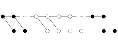
Figure 1: The cockroach graph from Guattery and Miller [26] has 80 nodes as illustrated above with each suspension points representing a line of 16 nodes. Here, we apply the fourth eigenvector to get this special partition where black for nodes of negative eigenvector values, white for positive ones. It’s easy to see that $w_{4}$ reaches its maximum when nodes with the same signs are in the same groups, while the graph structure tells us negative nodes are divided into three unconnected parts.

Hence, instead of clustering nodes as in Eq.(12), we add a natural constraint that each group should be a connected subgraph referring to the graph geometry structure. The square operation in Eq.(8) suggests that two operations on subgraphs are preferred: (a) nodes within the same subgroup share the same sign in $f_{j}$; (b) each subgroup contains as many nodes as possible. This consideration leads us to focus on partitions deduced according to the signs of each eigenvectors’ elements.

An interesting result named the Courant-Hilbert nodal theorem [7] gives a detail description about the domains cut by zeros of each eigenfunctions.

Given the self-adjoint second order differential equation $L[u]+\lambda\rho u=0$ ($\rho>0$) for a domain G with arbitrary homogeneous boundary conditions, if its eigenfunctions are ordered according to increasing eigenvalues, then the zeros of the $n$-th eigenfunction $u_{n}$ divide the domain into no more than $n$ subdomains. No assumptions are made about the number of independent variables. [From Courant-Hilbert: Methods in Mathematical Physics.]

It inspires us to take into account the corresponding discrete situation, which is the discrete nodal domain theorem on graph $G=(V,E)$. We define a positive (negative) strong nodal domain of a function $f$ on $V(G)$ to be a maximal connected induced subgraph of $G$ on vertices $v\in V$ with $f(v)>0$ $(f(v)<0)$. Meanwhile, a positive (negative) weak nodal domain of a function $f$ on $V(G)$ is a maximal connected induced subgraph with $f(v)\geq 0$ ($f(v)\leq 0$) that contains at least one nonzero valued node. The relation between eigenvectors and nodal domains was introduced and studied by Davies, Gladwell, Leydold, Stadler, et al. [6, 12]. One of those important results is

Theorem 2.1.

[6] Let $M$ is a symmetric matrix with nonnegative diagonal entries and $M_{uv}<0$ as $u\sim v$. Let $\lambda_{1}\leq\cdots<\lambda_{k}=\lambda_{k+1}\cdots=\lambda_{k+r-1}<\lambda_{k+r}\leq\cdots\leq\lambda_{n}$ be eigenvalues of $M$ and $f_{k}$ be the corresponding eigenvector of $\lambda_{k}$. Then, the number of strong nodal domains of $f_{k}$ is no more than $k+r-1$, and the number of weak nodal domains of $f_{k}$ is no more than $k$.

This theorem defines the matrix $M$ in a general expression, in which the Laplacian of graph is included. It shows a possible natural structure framework in which we achieve a maximization of $w_{j}$ satisfying the connectivity information. An interesting viewpoint occurs when there are zero elements in the eigenvectors. Weak nodal domains request a sharing of these nodes, which means an overlapping structure might be naturally defined, or certain basic functional parts in the dynamic system of the network are discovered.

3 Partition by weak nodal domain

Specially, eigenvector affording the second smallest eigenvalue of Laplacian of the network is called the Fiedler vector [18]. It has been applied in graph bi-partitioning [44] and spectral clustering [5]. Generally speaking, these methods provide partitions that attract rather large weight on the smallest nonzero eigenvalue in Eq.(9) to make $Cut(A_{1},\cdots,A_{k})$ small. However, bad results can be found upon many graphs in [26]. Take “cockroach graph” [26] for example, the second eigenvector offers a division horizontally cutting through the ladder while, obviously, the ideal cut is the long dots line (see Fig.2.(a)).

The discrete nodal domain theorem indicates that the Fiedler vector decides weak nodal domains no more than two, but for the cockroach graph, the ideal cut separates the graph into three parts. Spontaneously, we are interested in the behavior of the third eigenvector. Calculation shows that it provides the exact separation just as the ideal cut does (see Fig.2.(b)).

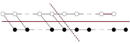
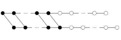
Figure 2: The cockroach graph from Guattery and Miller[26], where black for negative eigenvector nodes, white for positive eigenvector nodes. (a) the horizontal cutting is deduced by the second eigenvector, the dashes line implies the ideal separation; (b) partition deduced by the third eigenvector.

This result leads us back upon Eq.(9). Despite the weight expression $w_{j}=\sum_{l=1}^{k}(f_{j}^{T}S_{l})^{2}$, eigenvalues also play an important role in the minimization of the formula. Actually cockroach graph possesses two eigenvalues $\lambda_{2}=0.0057$ and $\lambda_{3}=0.0062$ that are relatively close, compared with $\lambda_{4}=0.0246$ and other eigenvalues, which implies that heavy weight on $\lambda_{3}$ is also a possible optimized choice. Hence, we can apply the eigenvectors other than the Fiedler vector to partition and this is so called the weak-nodal-domain partition(WNDP).

In most situations eigenvectors corresponding to smaller eigenvalues provide WNDP with smaller cut size, which makes multi-communities structure uneasy to be determined. To avoid this shortage, we take the famous quality function modularity $Q$ [41] as a criterion.

$$Q=\text{Tr}(S^{T}(A-P)S).$$

where $P$=($P_{ij}$) is the random configuration correspondence of $A$ satisfying $P_{ij}=\frac{d_{i}d_{j}}{2|E|}$ [41].

This quality function depicts the difference between how many edges within communities and how many edges to be expected within communities. Interestingly, we have

$$Q = \text{Tr}(S^{T}((D-P)-(D-A))S)$$

$$= \text{Tr}(S^{T}(D-P)S)-\text{Tr}(S^{T}(D-A)S),$$

where the first half represents expected edge number outside communities and the other half dedicates actual edge number of such set. Note that the second half is exact the cut size of the network mentioned before. We are interested in the difference between WNDP and the exact optimization result of modularity $Q$.

Consider a WNDP, $Q$ will be improved in three ways:

(i)two communities merge together: volume to be $V_{i}=\sum_{h\in A_{i}}d_{h}$ and $V_{j}=\sum_{h\in A_{j}}d_{h}$, number of connecting edges to be $c_{ij}$, this alteration only happens when

$$\frac{V_{i}*V_{j}}{2|E|}<c_{ij};$$

(ii)one community split into two: with the same definition as above, this alteration only happens when

$$\frac{V_{i}*V_{j}}{2|E|}>c_{ij};$$

(iii)move single vertex from one community to another: as vertex v with $n_{i}$ connections to $A_{i}$ and $n_{j}$ connections to $A_{j}$, it belongs to $A_{i}$ to make better benefit on $Q$ when

$$\frac{V_{i}*n_{i}}{2|E|}-\frac{V_{j}*n_{j}}{2|E|}<n_{i}-n_{j}.$$

The first two operations usually will not be needed if the community structure are relatively clear (see samples below), thus slight alterations on vertices may lead to a good approximation.

This algorithm is practically under processing in the form of matrix calculation. Specially, given the function $f$, the complexity of finding the weak nodal domains is $O(|V|)$.

Remember that there could be zero elements in the eigenvectors. Define a vertex $v$ to be a zero vertex if $f(v)=0$. Similarly a zero component is a maximal connected subgraph of zero vertices. We preprocess the graph in following steps:

(i)Contract all zero components into single vertices which inherit the connection of the components. Here, multiple edges are allowed. This leads to graph $G_{1}$.

(ii)Split each zero vertex in $G_{1}$, say $v$, into two connected individual vertices $v^{+}$ and $v^{-}$, in which $v^{+}$ inherits all neighbors of v with positive values in $f$ and $v^{-}$ inherits corresponding negative parts. (note that either all neighbors of v are zero vertices or all v has neighbors of different signs). This leads to graph $G_{2}$.

We call the new graph $G_{2}$ after the two steps a weak domain graph. It is the graph our algorithm be applied on. Note that the most complex part of the method is to calculate the eigenvectors of the sparse Laplacian matrix, which is known to be polynomial of order $O(n^{2})$, and one can apply shifted power method to get the the k-th eigenvector which is of complexity $O(\frac{n}{\log(\lambda_{k}-\lambda_{k-1})})$.

Situation with zero components could be complicated, for that modularity is defined on structure without overlapping. In this paper, a limitation of the definition on zero value to be of order $O(10^{-17})$ will avoid overlapping structure. The ambiguous boundaries will be discussed in our further work.

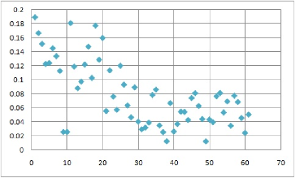
(a) Modularities of WNDPs by different eigenvectors of Laplacian on Dolphin graph. WNDP by $f_{2}$ is the best choice.

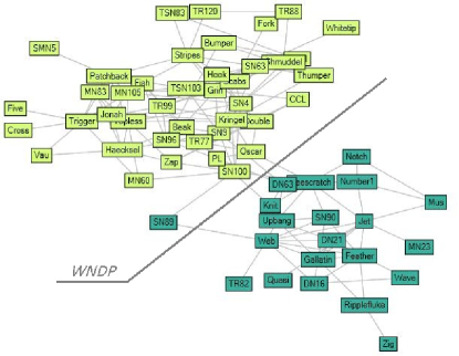
(b) The colors represent real observed division of 62 bottlenose dolphins. The solid line represents the result of WNDP. Follow our algorithm comes a partition with only one controversial node.

Figure 3: The Dolphin Graph [33]

4 Experiments with WNDP

The whole comparison framework define above allows us to test the best partition as well as reasonable number of clusters. Or more precisely, we are trying to find out what information the eigenvectors might suggest for a possible partition. Here, three different networks are conducted under our algorithm to test the WNDP method.

4.1 Dolphin Graph

The establishment of Dolphin graph [33] is based on certain group of bottlenose dolphins living in Doubtful Sound, New Zealand. The pattern that two dolphins getting alone together suggests certain relation among members of this representative animal social network. See Fig.3(b) for the detail connections. Scientists found an interesting phenomenon after years of observation: the whole group of dolphins split into two small subgroups following the departure of one key member named ’SN89’. This observed division is represented with colors in the figure.

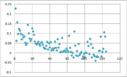
(a) Modularities of WNDPs by different eigenvectors of Laplacian on Political Books graph. WNDP by $f_{2}$ is selected by the algorithm.

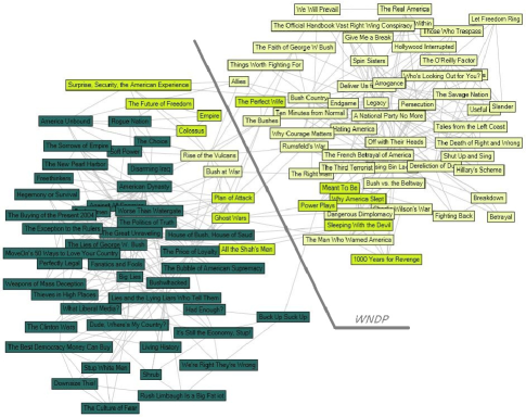
(b) Books with dark color are liberal, the grey ones are centrist or unaligned, and the rests without colors are conservative. The grey books act as buffers between the ones with left-wing and right-wing points of view. Solid line divides the graph following WNDP of $f_{2}$. Only two confused nodes representing books purchased frequently by both sides are positioned incorrectly.

Figure 4: The Political Books graph [32]

We process the graph with our algorithm, and the outcome indicates $f_{2}$ possessing reasonable WNDP(see Fig.3(a)). Solid line in Fig.3 depicts the division of the calculation result. Only ’SN89’ does not fit the real statement. The background of this division tells us ’SN89’ is an ambiguous node for its role as a association between two subgroups. Thus, the result of our method is quite close to the reality.

4.2 Political Books Graph

Political Books graph is assembled and studied by Krebs [32]. The database was taken from the online bookseller www.amazon.com, in which 105 books have been considered. Edges between books represent frequent co-purchasing by the same buyers. Krebs collected these information in 2004 around the US Election. He wanted to study the relation between books describing different political views. Naturally, this special graph inherits bilateral structure arising from the two different political tendency in the United States, democratic and republic respectively.

It is not surprising that WNDP by $f_{2}$ of Political Books graph reaches its optimum modularity. Fig.4(b) is the exact partition, in which each side has its particular groups of authors and readers. An intuitive survey of the original graph shows our prediction still has two books of liberal presented in the group of conservative.

4.3 Capocci Graph

Capocci Graph is a simple graph (as shown in Fig.6 up-left) generated by Capocci for the application of eigenvector component to identify communities [8]. The experiment shows that the second eigenvector of the right stochastic matrix, which is $D^{-1}A$, indicates three plateaus corresponding to the three evident component of the graph.

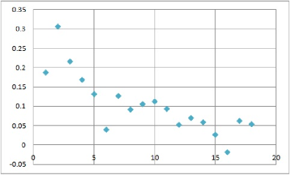
Figure 5: Modularities of WNDPs by different eigenvectors of Laplacian on Capocci graph, among which $f_{3}$ suggests the best choice.

Fig.5 depicts the numerical result of our algorithm that the largest modularity is offered by $f_{3}$. Detail partition is represented in Fig.6(a), in which we also demonstrate respectively the WNDPs of eigenvectors corresponding to the first three nonzero eigenvalues. Obviously, WNDP on the bottom-left by the chosen $f_{3}$ gives a partition matching our visual observation.

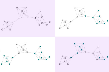
(a) up-left: the original graph; up-right: partition by $f_{2}$; bottom-left: partition by $f_{3}$; bottom-right: partition by $f_{4}$. Generally speaking, eigenvectors other than these four above would possess more complicated nodal domain structures.

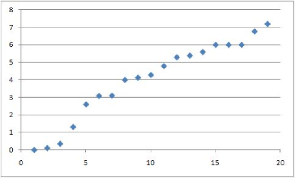
(b) The eigenvalues of the Laplacian on Political Books graph. Note that the first three eigenvalues are rather smaller than the rests.

Figure 6: The Capocci Graph [8]

Compared with Dolphin Graph and Political Books Graph, the best WNDP of Capocci Graph is the one according to $f_{3}$ other than $f_{2}$. This small alternation reminds us of the important roles that eigenvalues $\{\lambda_{j}\}$ have played in Eq.(9). To illustrate this idea, we separate small eigenvalues with relatively large ones

$$\sum_{j=2}^{n}\lambda_{j}w_{j}=\sum_{j=2}^{s}\lambda_{j}w_{j}+\sum_{j=s+1}^{n}\lambda_{j}w_{j}.$$

where $\{\lambda_{i}\}_{i=1}^{s}$ represent relatively small eigenvalues while $\{\lambda_{i}\}_{i=s+1}^{n}$ the large ones. Our experiments suggest that eigenvectors corresponding to $\{\lambda_{i}\}_{i=1}^{s}$ may hold the information about the community structure of the graph.

4.4 Computer-Generated Graphs

Take a rough look at the community structure, we contract each cluster of the WNDP into one single node inheriting connections of the cluster. Despite multiple edges, no circles exit in this simple structure which, in brief, is a tree. This interesting phenomenon comes from the fact that only two signs ‘+‘ and ‘-‘ are used to identify different nodes. We generate a graph artificially following the method used by Girvan and Newman [27], also called the ad hoc network, in which a whole graph of 128 vertices is divided into four communities of 32 vertices each. More precisely, in our special case, edges between pairs of nodes in the same community are placed with possibility 0.4 while ones in different communities share possibility 0.1. The randomness of the edges indicates multiple choices, however, we are only interested in the known community structure of these graphs. Graph in Fig.7 is one of these special samples following the Girvan and Newman’s method on which our algorithm is applied on. It is easy to find out that at least four signs are required to separate these four communities, which suggests our method being incomplete.

Calculation shows that WNDPs by eigenvectors according to the first three nonzero eigenvalues divide the graph into two parts respectively (see Fig.7). In other words, each eigenvector reveals part of the community structure. By combining these partial information together, we may recover the acknowledge of the whole structure. This leads us to a generalized definition of the nodal domains: a strong nodal domain of functions $\{f_{1},\cdots,f_{i}\}$ on $V(G)$ is a maximal connected induced subgraph of $G$ on vertices $v\in V$ which have corresponding vectors $(f_{1}(v),\cdots,f_{i}(v))$ belonging to the same quadrant of the i-dimension Euclid space. Note that ’i’ is the exact number of eigenvectors $\{f_{1},\cdots,f_{i}\}$ on which we process for the combined information. So is the alteration about the definition of weak nodal domains.

Figure 7: The artificial sample assembled by computer. The four communities are easily recognized through direct observation. The color shade represents different clusters which are suggested by the eigenvectors. Small graphs on the top are separated by WNDPs corresponding to the second and fourth eigenvectors respectively, in which only two clusters each are detected. Combination of these two results reveals the exact community structure, and they are exact the mathematical outcome of generalized WNDP.

Convictive result comes out by applying our algorithm on these generalized WNDP (see Fig.7). Single eigenvector does separate the whole network into reasonable parts, but not subtly enough. Structure functioning with a relatively small scale will be demonstrated by appropriate blend of certain eigenvectors.

5 Conclusion

The experiments above confirm that the nodal domains of the Laplacian eigenvectors do hold certain information about the community structure of the graph. Still, exception would arise when the situation comes with relatively large difference between the volume numbers of communities. Virtually, we set up a graph with following three steps (see Fig.8):

• Use ER model [15] to build a graph, named $G_{1}$, of 200 nodes whose average degree is 40 (nodes shaped in solid squares).

• Use ER model to build another graph, named $G_{2}$, of 20 nodes whose average degree is 4 (nodes shaped in solid circles).

  

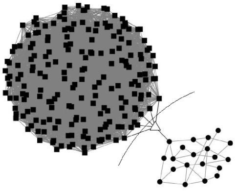
  Figure 8: This special graph is established by following the three steps above. The triangle in the figure is the key contradiction. Solid line divides the graph by WNDP while direct observation shows the triangle is placed incorrectly.

• Build an extra single node, first connect it with a random node in $G_{2}$, then connect it with five random nodes in $G_{1}$ (node shaped in triangle).

Calculation suggests that WNDP by the second eigenvector possesses the largest modularity. Solid line in Fig.8 shows the exact division. But direct observation tells us the triangle has more connection with $G_{1}$ than that with $G_{2}$.

A survey into the algorithm knowledged us that the process of calculating the eigenvectors is equal to evaluate each point with a average of its neighbor’s eigenvector value, but under a certain rate which is the eigenvalue. Thus, the eigenvector $f_{2}$ of the Laplacian on the graph would evaluate nodes in $G_{1}$ with positive values while negative ones for $G_{2}$. Because $G_{2}$ has much less nodes than $G_{1}$, $f_{2}$ on $G_{2}$ possess relatively small negative values, which indicates that under the mean of average the triangle could have a negative value as nodes in $G_{2}$ do. Further work should be focused on the position amendment of the boundary nodes like the triangle.

In section III, we already find this situation a solution by checking the boundary vertices for improvement on modularity $Q$. But recall the first two operations in modifying $Q$, we note that if the volume of the two communities is small or unbalanced(with wide gap), these two should not be separated for the inequality being unsatisfied. That is why the modularity has a well-known resolution limit, that makes clusters smaller than a given size undetectable. A resolution coefficient $\lambda$ is welcome to make up this limitation as the inequality goes as

$$\frac{V_{i}*V_{j}}{2\lambda|E|}<c_{ij},\lambda\in(0,1]$$

where the vertexes are localized that we only consider the influence form their ranged neighbours.

To conclude, in this paper we introduce the method that applies weak nodal domains according to eigenvectors of the Laplacian on the graph. We calculate modularity [40, 41] to decide which WNDP behaves best that it may suggest the optimal number of communities in networks. We also test our algorithm in real-world models. As the examples show, for arbitrary graphs, WNDP works quite well in deciding the number of clusters in the graphs. For un-weighted graph the mechanism why the WNDP works so good is still unknown, and we will work on this in our future study as well as finding other good parameters to choose the best eigenvectors.

References

- [1] A.-L. Barabási and R. Albert, Science 286, 509-512 (1999).
- [2] R. Albert, H. Jeong, and A.-L. Barabási, Nature 401, 130-131 (1999).
- [3] M.A. de Menezes and A.-L. Barabási, Phys. Rev. Lett. 93, 068701 (2004).
- [4] P. Bonacich, The American Journal of Sociology, 92(5),1170-1182 (1987).
- [5] M. Belkin and P. Niyogi, In Advances in Neural Information Processing Systems 14 (NIPS 2001), 585-591, (Cambridge, MIT Press, 2002).
- [6] T. Biyikoglu, J. Leydold and P. F. Stadler, in Lecture notes in mathematics Springer, (2007).
- [7] R. Courant, D. Hilbert. Methods of mathematical physics, (Vol. 1, John Wiley & Sons, 1989).
- [8] A. Capocci, V. D. P. Servedio, G. Caldarelli, and F. Colaiori, In S. Leonardi (ed.), Proceedings of the 3rd Workshop on Algorithms and Models for the Web Graph, number 3243 in Lecture Notes in Computer Science, (Springer, Berlin, 2004).
- [9] F. Chung, Spectral Graph Theory, (AMS Publications, 1997).
- [10] F. Chung and L. Lu, Ann. Comb. 6, 125 (2002).
- [11] D. M. Cvetković, P. Rowlinson, and S. Simić, volume 66 of Encyclopdia of Mathematics and its Applications. (Cambrigdge University Press, Cambridge, UK, 1997).
- [12] Yael Dekel, James R. Lee, Nathan Linial, In Proceedings of APPROX-RANDOM’2007, pp.436 448.
- [13] D.J. Watts and S.H. Strogatz, Nature 393, 440-442 (1998).
- [14] Z. Dezsö, E. Almaas, A. Lukács, B. Rácz, I. Szakadát, and A.-L. Barabási, Phys. Rev. E 73, 066132 (2006).
- [15] P. Erdös and A. Rényi, Publ. Math. (Debrecen) 6, 290-297, (1959).
- [16] T. Li, J. Liu and W. E, Phys. Rev. E 80, 026106 (2009).
- [17] W. E, T. Li, and E. Vanden-Eijnden, Proc. Natl. Acad. Sci. U.S.A. 105, 7907 (2008).
- [18] M. Fiedler, Czech. Math. J. 23, 298-305 (1973).
- [19] L. C. Freeman, Sociometry 40, 35 (1977).
- [20] L. C. Freeman, Social Networks, 1(3), 215-239 (1979).
- [21] S. Fortunato, V. Latora, and M. Marchiori, Phys. Rev. E 70, 056104 (2004).
- [22] M. Faloutsos, P. Faloutsos, and C. Faloutsos, Comput. Commun. Rev. 29, 251 (1999).
- [23] D. A. Fell and A. Wagner, Nature Biotechnology 18, 1121-1122 (2000).
- [24] R. Guimerà and L. A. N. Amaral, Nature (London) 433, 895 (2005).
- [25] M. Granovetter, The American Journal of Sociology, 78, 1360-1380 (1973).
- [26] S, Guattery and G, Miller, SIAM Journal of Matrix Anal. Appl., 19(3), 701-719 (1998).
- [27] M. Girvan and M. E. J. Newman, Proc. Natl. Acad. Sci. USA 99, 7821-7826 (2002).
- [28] J. Q. Jiang, A. W.M. Dress, G. Yanga, Appl. Math. Let. 22, 1479-1482 (2009).
- [29] H. Jeong, B. Tombor, R. Albert, Z. N. Oltvai, and A.-L. Barabási, Nature 407, 651-654 (2000).
- [30] B. W. Kernighan and S. Lin, Bell System Technical Journal 49, 291-307 (1970).
- [31] K.A. Stephenson and M. Zelen, Social Networks 11, 1-37 (1989).
- [32] V.Krebs (unpublished) see: http://www.orgnet.com/.
- [33] D. Lusseau, K. Schneider, O. J. Boisseau, P. Haase, E. Slooten, and S. M. Dawson, Behav. Ecol. Sociobiol. 54, 396 (2003).
- [34] Ulrike von Luxburg, Statistics and Computing, Vol.17, No.4, pp.395-416 (2007).
- [35] R. Merris, Lin. Algebra Appl. 278, 221-236 (1998).
- [36] C. Moore and M. E. J. Newman, Phys. Rev. E 61, 5678 (2000).
- [37] M. Molloy and B. Reed, Random Structures and Algorithms, 6, 161-180 (1995).
- [38] M. E. J. Newman, Proc. Natl. Acad. Sci. U.S.A. 98, 404 (2001).
- [39] M. E. J. Newman and M. Girvan, Phys. Rev. E 69, 026113 (2004).
- [40] M. E. J. Newman, Eur. Phys. J. B 38, 321-330 (2004).
- [41] M. E. J. Newman, Phys. Rev. E 74, 036104 (2006).
- [42] M. E. J. Newman, Proc. Natl. Acad. Sci. U.S.A. 103, 8577 (2006).
- [43] R. Pastor-Satorras and A. Vespignani, Phys. Rev. Lett. 86, 3200 (2001).
- [44] A. Pothen, H. Simon, and K.-P. Liou, SIAM J. Matrix Anal. Appl. 11, 430-452 (1990).
- [45] S. Redner, Eur. Phys. J. B 4, 131 (1998).
- [46] G. Sabidussi, The centrality index of a graph. Psychometrika, 31 (4), 581-603 (1966).
- [47] R. S. Weiss and E. Jacobson, American Sociological Review, 20,661-668 (1955).
- [48] W.E. Donath and A.J.Hoffman, IBM J. Res. Develop., 17, 420-425 (1973).