Constructing a chaotic system with any number of equilibria

Abstract

In the chaotic Lorenz system, Chen system and Rössler system, their equilibria are unstable and the number of the equilibria are no more than three. This paper shows how to construct some simple chaotic systems that can have any preassigned number of equilibria. First, a chaotic system with no equilibrium is presented and discussed. Then, a methodology is presented by adding symmetry to a new chaotic system with only one stable equilibrium, to show that chaotic systems with any preassigned number of equilibria can be generated. By adjusting the only parameter in these systems, one can further control the stability of their equilibria. This result reveals an intrinsic relationship of the global dynamical behaviors with the number and stability of the equilibria of a chaotic system.

PACS: 05.45.-a, 05.45.Ac, 05.45.Pq

Thus far, one typically calculates the number and determines the corresponding stability of the equilibria of a given chaotic system, but seldom considers how to generate a desirable chaotic system with a preassigned number and preferred stability of equilibria. This article shows that, for 3D autonomous systems, the latter can be done effectively in a fairly simple way. This helps better understand the intrinsic relationship between the equilibria and dynamics of a chaotic system.

I Introduction

In chaos theory, it is important to study the stability of the equilibria of an autonomous dynamical system. For a dynamical system described by a set of autonomous ordinary differential equations (ODEs), $\dot{\textbf{x}}=f(\textbf{x}),\,\textbf{x}\in R^{n}\$, if $f(\textbf{x}_{\rm e})=0$ has real solution then $\textbf{x}_{\rm e}$ is called the equilibrium  of this dynamical system. An equilibrium is said to be hyperbolic  if all eigenvalues of the system Jacobian matrix have non-zero real parts. A hyperbolic equilibrium for three-dimensional (3D) autonomous system can be a node, saddle, node-focus  or saddle-focus. For 3D autonomous hyperbolic type of dynamical systems, a commonly accepted criterion for proving the existence of chaos is due to Ši’lnikov Silinkov1 ; Silinkov2 ; Silinkov3 ; Silinkov5 ; Silinkov6chenEXTENDED .

It has also been noticed that although most chaotic systems are of hyperbolic type, there are still many others that are not so. For non-hyperbolic type of chaotic systems, they usually do not have saddle-focus equilibria, such as those found by Sprott sprott1993 ; sprott1994 ; sprott1997 ; sprottlinz2000 .

The well-known Lorenz system lorenz63 and also Chen system chen1999 ; ueta2000 both have two unstable saddle-foci and one unstable node. They can generate a two-wing butterfly-shaped chaotic attractor. Near the center of the two wings, there lies one an unstable saddle-focus. In recent years, some chaotic systems are found which can generate three-wing, four-wing, and even multi-wing attractors. Observe that, typically, for those symmetrical four-wing attractors, near the center of their wings there also lies one unstable saddle-focus. This common feature may imply that the number of equilibria basically determines the shape of a multi-wing attractor. Therefore, it is interesting to ask: Is it possible to generate a chaotic system with an arbitrarily preassigned number of equilibria? Is the number of equilibria always determinate the shape of an attractor?

Furthermore, regarding the stability of the equilibria, recall that recently Yang and Chen found a chaotic system with one saddle and two stable node-foci yang2008 , and an unusual 3D autonomous quadratic Lorenz-like chaotic system with only two stable node-foci yang2010 . Moreover, Wang and Chen found an interesting chaotic system with only one stable node-focus onestable2011 . Thus, another interesting question is whether it is possible for a chaotic system to have two, or three, or even an arbitrarily large number of stable/unstable equilibria?

This paper attempts to answer these questions by showing a novel example of a chaotic system with no equilibrium, and several other examples of chaotic systems which have any preassigned number of equilibria. Meanwhile it is shown that, by adjusting the only parameter in these systems, one can also control the stability of these equilibria.

II Chaotic system with no equilibrium

First, a 3D chaotic autonomous system system is introduced:

$$\left\{\begin{array}[]{l}\dot{x}=y\\ \dot{y}=z\\ \dot{z}=-y+3y^{2}-x^{2}-xz-a\,,\end{array}\right.$$ (1)

Figure 1: (Color online) The chaotic attractor of system (1), which has two symmetrical equilibria when $a=0.01$: 3D views on the $x$-$y$ plane, $x$-$z$ plane and $y$-$z$ plane.

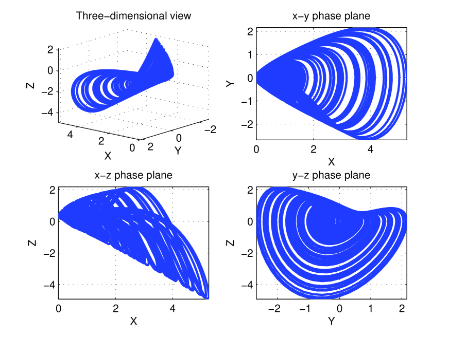
Figure 2: (Color online) The chaotic attractor of system 1, which has no equilibrium when $a=-0.05$; 3D views on the $x$-$y$ plane, $x$-$z$ plane and $y$-$z$ plane.

Figure 3: (Color online) The largest Lyapunov exponent of system (1) with respect to the parameter $a$.

When $a>0$, this system has two symmetrical equilibria: $(\sqrt{a},0,0)$ and $(-\sqrt{a},0,0)$, as shown by Fig. 1. When $a=0$, these two symmetrical equilibria merge into one, the origin $(0,0,0)$. When $a<0$, there is no equilibrium in this system, but still, the system can generate a chaotic attractor, as shown in Fig. 2. The largest Lyapunov exponent with respect to the parameter $a$ is shown in Fig. 3, which convincingly implies that the system is chaotic.

III A modified Sprott E system with one stable equilibrium

Now, a chaotic system with only one equilibrium, a stable node-focus, is introduced, which was reported in onestable2011 .

This system was found by modifying the Sprott E system, as follows:

$$\left\{\begin{array}[]{l}\dot{x}=yz+a\\ \dot{y}=x^{2}-y\\ \dot{z}=1-4x\,.\end{array}\right.$$ (2)

When $a=0$, it is the Sprott E system sprott1997 ; when $a\neq 0$, however, the stability of the single equilibrium is fundamentally different.

Specifically, when $a>0$, system (2) possesses only one stable equilibrium:

$$P\left(x_{E},y_{E},z_{E}\right)=\left(\frac{1}{4},\frac{1}{16},-16\,a\right)\,.$$ (3)

Figure 4: (Color online) The chaotic attractor of system (2), when $a=0.006$; 3D views on the $x$-$y$ plane, $x$-$z$ plane and $y$-$z$ plane.

Some numerical calculation results are shown in Table 1.

Table 1: Jacobian eigenvalues of system (2)

$a$	Jacobian eigenvalues
$0$	$-1$,$\pm 0.5i$
$0.006$	$-0.9607$, $-0.0197\pm 0.5098i$
$0.022$	$-0.8458,-0.0771\pm 0.5382i$

Interestingly, this system (2) can generate a one-scroll chaotic attractor, as shown in Fig. 4.

In the following, this system (2) is further modified by imposing some kind of symmetry onto it, to have different numbers of equilibria while keeping this system chaotic.

IV Chaotic system with two equilibria

Rewrite system (2) in terms of $u,v,w$ as follows:

$$\left\{\begin{array}[]{l}\dot{u}=vw+a\\ \dot{v}=u^{2}-v\\ \dot{w}=1-4u\,.\end{array}\right.$$ (4)

From Fig. 4, one can see that the $y$-axis does not intersect with the attractor in system (2). So, one may try to add a $y$-axis rotation symmetry to this system, as detailed below.

Consider the following simple coordinate transformation:

$$\left\{\begin{array}[]{l}u=x^{2}-z^{2}\\ v=y\\ w=2xz\,.\end{array}\right.$$ (5)

This transformation can add a $y$-axis rotation symmetry, $\mathbb{R}_{y}(\pi)$, to the original system, because for each $(u,v,w)$ there are two points $(\pm x,\pm y,\pm z)$ corresponding to $(u,v,w)$.

After the above transformation, the system becomes

$$\left\{\begin{array}[]{l}\dot{x}=\frac{1}{2}{\frac{z+2y{x}^{2}z+xa-4{x}^{2}z+4{z}^{3}}{{x}^{2}+{z}^{2}}}\\ \dot{y}=\left({x}^{2}-{z}^{2}\right)^{2}-y\\ \dot{z}=-\frac{1}{2}{\frac{2yx{z}^{2}+za-4x{z}^{2}-x+4{x}^{3}}{{x}^{2}+{z}^{2}}}\,.\end{array}\right.$$ (6)

The new system (6) possesses two symmetrical equilibria, which are independent of the parameter $a$: $P1(\frac{1}{2},\frac{1}{16},0)$ and $P1(-\frac{1}{2},\frac{1}{16},0)$.

System (6) is not globally but only locally topologically equivalent to the original system (2), however. Yet one can control the stability of these equilibria by adjusting the parameter $a$, so that the stability remains the same as the original system (2) which, when $a<0$ are unstable and when $a>0$ are stable.

By linearizing system (2) at $P1(\frac{1}{2},\frac{1}{16},0)$, one obtains the Jacobian

$$J\,\Big{|}_{O}=\left[\begin{array}[]{ccc}-2a&0&\frac{1}{16}\\ \frac{1}{2}&-1&0\\ -4&0&-2a\\ \end{array}\right]\,,$$ (10)

whose characteristic equation is

$${\rm det}(\lambda I-J|_{O})=\lambda^{3}+(1+4a)\lambda^{2}+\Big{(}4a^{2}+4a+\frac{1}{4}\Big{)}\lambda+4a^{2}+\frac{1}{4}=0\,,$$

which yields

$$\lambda_{1} = -1<0,$$

$$\lambda_{2} = -2a+0.5i,$$

$$\lambda_{3} = -2a-0.5i\,.$$

System (6) can generate a symmetrical two-petal chaotic attractor, as shown in Fig. 5 and Fig. 6, respectively.

Numerical calculation of the largest Lyapunov exponent of the the system indicates the existence of chaos for some particular values of parameter $a$, as shown in Fig. 7.

Figure 5: (Color online) The new two-petal chaotic attractor with stable equilibria when $a=0.003$.

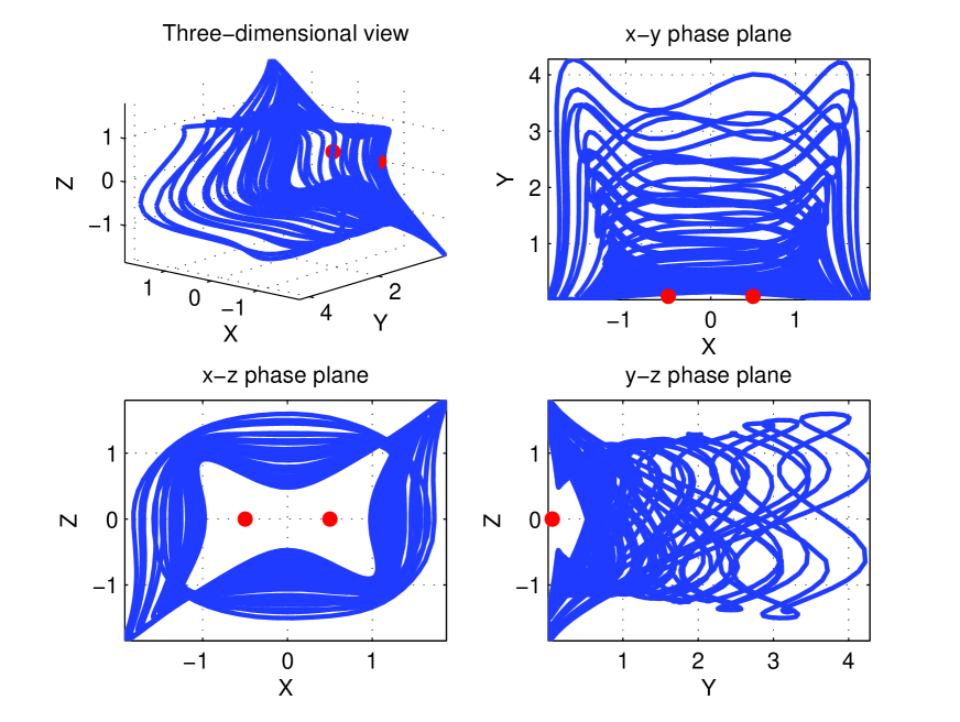
Figure 6: (Color online) The new two-petal chaotic attractor with unstable equilibria when $a=-0.01$.

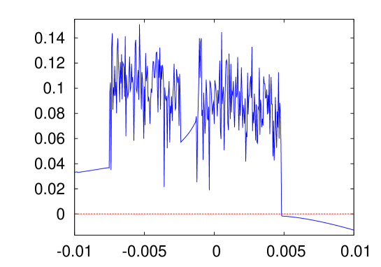
Figure 7: (Color online) The largest Lyapunov exponent of system (6) with respect to parameter $a$.

V Chaotic system with three equilibria

Similarly, consider the following transformation:

$$\left\{\begin{array}[]{l}u=x^{3}-3xz^{2}\\ v=y\\ w=3x^{2}z-z^{3}\,.\end{array}\right.$$ (11)

It can add a $y$-axis rotation symmetry, $\mathbb{R}_{y}(\frac{2}{3}\pi)$, to the original system, because for each $(u,v,w)$ there are three symmetrical points corresponding to it.

After the above transformation, the system becomes

$$\left\{\begin{array}[]{l}\dot{x}=\frac{1}{3}{\frac{3\,{x}^{4}zy-4\,{x}^{2}{z}^{3}y+{x}^{2}a-8\,{x}^{4}z+2\,zx+24\,{x}^{2}{z}^{3}+{z}^{5}y-{z}^{2}a}{2\,{x}^{2}{z}^{2}+{x}^{4}+{z}^{4}}}\\ \dot{y}=(x^{3}-3xz^{2})^{2}-y\\ \dot{z}=-\frac{1}{3}{\frac{6\,{z}^{2}{x}^{3}y-2\,{z}^{4}xy+2\,zxa+4\,{x}^{5}-{x}^{2}-16\,{z}^{2}{x}^{3}+{z}^{2}+12\,{z}^{4}x}{2\,{x}^{2}{z}^{2}+{x}^{4}+{z}^{4}}}\,.\end{array}\right.$$ (12)

This system possesses three symmetrical equilibria, which are dependent on the parameter $a$. The analytical expression are too long to write out here, so only some numerical results are shown in Table 2.

Table 2: Equilibria and Jacobian eigenvalues of system (12)

	$a$	Equilibria	Jacobian eigenvalues
Unstable case	$-0.01$	P1=(0.6550,0.0625,0.1258) P2=(-0.2186,0.0625,-0.6300) P3=(-0.4365,0.0625,0.5044)	$-1.0617,0.0308\pm 0.4843i$
Stable case	0.01	P1=(0.6550,0.0625,-0.1258) P2=(-0.2186,0.0625,0.6300) P3=(-0.4365,0.0625,-0.5044)	$-0.9334,-0.0333\pm 0.5165i$

The system has a symmetrical three-petal chaotic attractor, as shown in Fig. 8 and Fig. 9, respectively.

Numerical calculation of the largest Lyapunov exponent indicates the existence of chaos for some particular values of parameter $a$, as shown in Fig. 10.

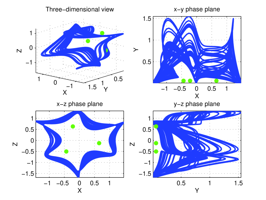
Figure 8: (Color online) Chaotic attractor of system (12) with three stable symmetrical equilibria when $a=0.01$.

Figure 9: (Color online) Chaotic attractor of system (12) with three unstable symmetrical equilibria when $a=-0.01$.

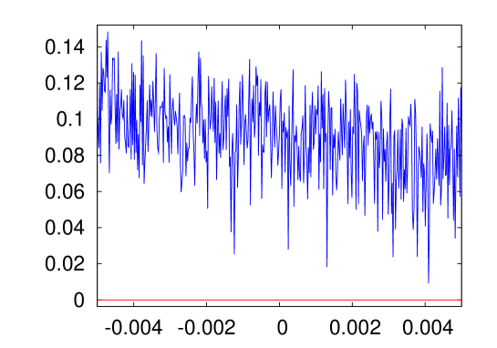
Figure 10: (Color online) The largest Lyapunov exponent of system (12) with respect to the parameter $a$.

VI Chaotic system with any number of equilibria

Theoretically, one can use the transform $(x+iz)^{n}=(u+iv)$ to obtain a new chaotic system with $n$ equilibria. The following is such an example with five equilibria.

Consider the following transformation:

$$\left\{\begin{array}[]{l}u=x^{5}-10x^{3}z^{2}+5xz^{4}\\ v=y\\ w=5x^{4}z-10x^{2}z^{3}+z^{5}\,.\end{array}\right.$$ (13)

It can add a $y$-axis rotation symmetry, $\mathbb{R}_{y}(\frac{2}{5}\pi)$, to the original system. The new equations are too long to write out, so are omitted here. The symmetrical attractor generated with parameter $a=0$ is shown in in Fig. 11.

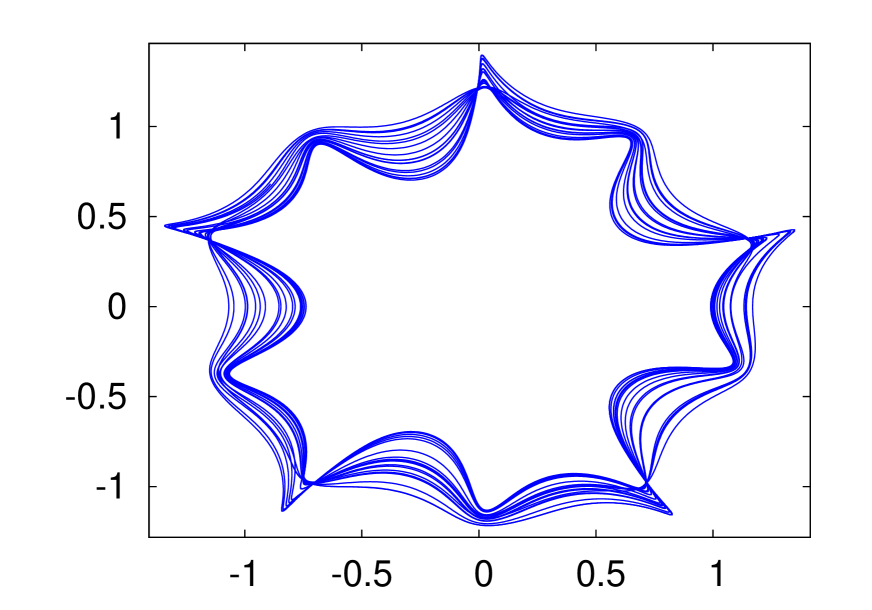
Figure 11: (Color online) Chaotic attractor of the new system with five symmetrical equilibria when $a=0$.

VII Discussions

The Hartman-Grobman Theorem is an important theorem in ODE systems theory. It is about the local  behavior of an autonomous dynamical system in the neighborhood of a hyperbolic equilibrium, stating that the behavior of the dynamical system near the hyperbolic equilibrium is qualitatively the same as (i.e., topologically equivalent to) the behavior of its linearization near this equilibrium point.

Notice, however, that the new systems discussed in this paper have chaos, which is a global  behavior, although such a system has only one hyperbolic equilibrium point. In other words, all system flows locally converge to the stable equilibrium, but they are chaotic globally. This interesting phenomenon is worth further studying, both theoretically and experimentally, to further reveal the intrinsic relationship between the local stability of an equilibrium and the global complex dynamical behaviors of a chaotic system.

References

- (1) L. Ovsyannikov and L. Šil’nikov. “On systems with a saddle-focus homoclinic curve”. Sbornik: Mathematics, 58(2): 557–574, 1987.
- (2) L. Šil’nikov. “A contribution to the problem of the structure of an extended neighborhood of a rough equilibrium state of saddle-focus type”. Sbornik: Mathematics, 10(1): 91–102, 1970.
- (3) A. Šil’nikov, L. Šil’nikov, and D. Turaev. “Normal forms and Lorenz attractors”. Int. J. Bifurcation Chaos, 3: 1123–1123, 1993.
- (4) L. Šilnikov, A. Šilnikov, and D. Turaev. Methods of Qualitative Theory in Nonlinear Dynamics. World Scientific Pub Co., Singapore, 2001.
- (5) B. Chen, T. Zhou, and G. Chen. “An extended šil’nikov homoclinic theorem and its applications”. Int. J. Bifurcation Chaos, 19: 1679–1693, 2009.
- (6) J. C. Sprott. “Automatic generation of strange attractors”. Comput. Graphics, 17: 325–332, 1993.
- (7) J. C. Sprott. “Some simple chaotic flows”. Phys. Rev. E, 50: 647–650, 1994.
- (8) J. C. Sprott. “Simplest dissipative chaotic flow”. Phys. Lett. A, 228: 271–274, 1997.
- (9) J. C. Sprott and S. J. Linz. “Algebraically simple chaotic flows”. J. Chaos Theory Appl., 5: 3–22, 2000.
- (10) E. N. Lorenz. “Deterministic nonperiodic flow”. J. Atmospheric Sci., 20: 130–141, 1963.
- (11) T. Ueta and G. Chen. “Yet another chaotic attractor”. Int. J. Bifurcation Chaos, 9: 1465–1466, 1999
- (12) T. Ueta and G. Chen. “Bifurcation analysis of Chen’s equation”. Int. J. Bifurcation Chaos, 10: 1917–1931, 2000.
- (13) Q. Yang and G. Chen. “A chaotic system with one saddle and two stable node-foci”. Int. J. Bifurcation Chaos, 18: 1393–1414, 2008.
- (14) Q. Yang, Z. Wei, and G. Chen. “An unusual 3D autonomous quadratic chaotic system with two stable node-foci”. Int. J. Bifurcation Chaos, 20: 1061–1083, 2010.
- (15) X. Wang and G. Chen. “A chaotic system with only one stable equilibrium”. Commun. Nonlinear Sci. Numer. Simul., 17(3): 1264-1272, 2012.