New variational Monte Carlo method with an energy variance extrapolation
for large-scale shell-model calculations

Abstract

We propose a new variational Monte Carlo (VMC) method with an energy variance extrapolation for large-scale shell-model calculations. This variational Monte Carlo is a stochastic optimization method with a projected correlated condensed pair state as a trial wave function, and is formulated with the $M$-scheme representation of projection operators, the Pfaffian and the Markov-chain Monte Carlo (MCMC). Using this method, we can stochastically calculate approximated yrast energies and electro-magnetic transition strengths. Furthermore, by combining this VMC method with energy variance extrapolation, we can estimate exact shell-model energies.

Shell-model calculations have been a central issue in studies of nuclear structure, and constant effort has been made to solve large-scale shell-model problems. Exact diagonalization, which is a standard method, has recently been able to handle large-scale problems with $O(10^{10})$ dimension caurier ; shimizu-okinawa . However, computational feasibility in this method is limited and strongly depends on the size of single particle space and valence nucleon numbers. To overcome this problem and to extend the feasibility of shell-model calculations, various methodssmmc ; dmrg ; vampir ; CCM ; qmcd ; mcsm ; exlanc ; papen ; exmcsm with different kinds of algorithms have been proposed and improved.

In this paper, we propose a new method for shell-model calculations using the Markov-chain Monte Carlo (MCMC). This new method is a variational Monte Carlo (VMC) with a projected correlated condensed pair state as a trial wave function. This new VMC can stochastically give not only energies but also electro-magnetic transition strengths, although these values are approximated. To estimate the exact shell-model energies over the limitations of variational formulation, we use the energy variance extrapolation, which has been studied in Refs.imada1 ; sorella and has been successfully applied to the nuclear shell model exlanc ; exmcsm . As this extrapolation needs a series of systematically approximated wave functions, we introduce a truncation scheme based on the spherical basis in the form of a projection operator.

In this study, projection operators are implemented by using the Monte Carlo in a novel way. In fact, particle number projection, magnetic quantum number projection, parity projection, and projection onto truncation spaces can be implicitly performed without numerical integrations, and angular momentum projection is performed by two-dimensional numerical integration.

Here we consider a new variational formulation of shell-model calculations. As a trial wave function for a nuclei with $N_{\pi}$ valence protons and $N_{\nu}$ valence neutrons, i.e., $N=N_{\pi}+N_{\nu}$, we take $|\psi\rangle$ as

$$|\psi\rangle=GP|\phi\rangle$$ (1)

and

$$|\phi\rangle=\left(\sum f_{kk^{\prime}}c_{k}^{\dagger}c_{k^{\prime}}^{\dagger}\right)^{N/2}|0\rangle$$ (2)

where $f$ is a skew-symmetric matrix. The $|0\rangle$ is an inert core and the $c_{i}^{\dagger}$’s are proton or neutron creation operators ($i=1,\cdots,N_{\pi}$ : proton and $i=N_{\pi}+1,\cdots,N$ : neutron). By this parametrization, proton-neutron pairing correlation is included, in addition to the proton-proton and neutron-neutron pairing correlations. For simplicity, to present this formulation, we assume that the components of $f$ are real numbers. We can also use a complex number although this would require some modifications. The $P$ is a projection operator and we use the following two kinds. One is

$$P=P^{I_{0}}P^{\pi}P_{M}$$ (3)

where $P^{I_{0}}$, $P^{\pi}$ and $P_{M}$ are projectors of the $z$-component of isospin $I_{0}$, parity $\pi$ and $z$-component of angular momentum $M$, respectively. The other is

$$P=P^{I_{0}}P^{\pi}P^{J}$$ (4)

where $P^{J}$ is a projection onto angular momentum $J$. The $G$ is a correlation factor as

$$G=e^{-\sum_{i\leq j}\alpha_{ij}n_{i}n_{j}}$$ (5)

where $\alpha$’s are variational parameters. The $n_{i}$ is taken as a number operator for orbit $i$, so that the $G$ is commutable with the angular-momentum projector. The $G$ can be easily evaluated as will be discussed later.

For the trial wave function in Eq.(1), the energy expectation value is given by

$$E=\langle H\rangle=\frac{\langle\phi\left|PGHGP\right|\phi\rangle}{\langle\phi\left|PGGP\right|\phi\rangle}.$$ (6)

To evaluate this, we introduce an alternative representation of the projection operator in Eq.(3), which can be shown by the so-called $M$-scheme states defined as

$$\left|m\rangle=c_{m_{1}}^{\dagger}c_{m_{2}}^{\dagger}\right.\cdots c_{m_{N}}^{\dagger}|0\rangle,$$ (7)

where $m=(m_{1},m_{2},\cdots m_{N})$. As the $M$-scheme state is an eigenstate of the $z$-components of the isospin and angular momentum, and parity, the projection operator is given by

$$P^{I_{0}}P^{\pi}P_{M}=\sum_{m\in\{M^{\pi}\}}|m\rangle\langle m|$$ (8)

where the summation is restricted within the $M$-scheme states with given quantum numbers, that is, particle numbers $N_{\pi}$ and $N_{\nu}$, and magnetic and parity quantum numbers $M$ and $\pi$. By this representation, $\langle m|P|\phi\rangle$ can easily be calculated as

$$\langle m|P^{I_{0}}P^{\pi}P_{M}|\phi\rangle=\langle m|\phi\rangle\delta_{z(m),M^{\pi}}$$ (9)

where $z(m)$ gives the parity and magnetic quantum numbers of the $M$-scheme state $|m\rangle$.

By introducing the $M$-scheme representation of the projection operator, the $G$-factor becomes a c-number because the $G$-factor is diagonal in the $M$-scheme, that is,

$$G|m\rangle=G(m)|m\rangle,$$ (10)

where the $G(m)$ is an expectation value of the $G$ concerning the $M$-scheme state $|m\rangle$. Moreover the matrix elements of the $H$ between $M$-scheme states can also be evaluated, and we denote them as

$$\langle m|H|m^{\prime}\rangle=h_{m,m^{\prime}}$$ (11)

where $|m\rangle$ and $|m^{\prime}\rangle$ have the same quantum numbers and $h$ is generally very sparse because a shell-model Hamiltonian consists of one-body and two-body interactions.

By these relations (10) and (11), Eq.(6) can be rewritten as

$$E=\sum_{m\in\{M^{\pi}\}}\rho(m)E_{L}(m),$$ (12)

where the local energy $E_{L}(m)$ is defined as

$$E_{L}(m)=\sum_{m^{\prime}\in\{M^{\pi}\}}h_{m,m^{\prime}}\frac{\langle m^{\prime}|P|\phi\rangle G(m^{\prime})}{\langle m|P|\phi\rangle G(m)},$$ (13)

and the sampling density $\rho(m)$ is defined by

$$\rho(m)=\frac{|\langle m|P|\phi\rangle G(m)|^{2}}{\sum_{m\in\{M^{\pi}\}}|\langle m|P|\phi\rangle G(m)|^{2}},$$ (14)

where $\rho(m)\geq 0$ and $\sum_{m\in\{M^{\pi}\}}\rho(m)=1$.

In numerical calculations, the energy formula Eq.(12) is not practical because the dimension of the $M$-scheme space becomes intractably huge as the size of single particle space and proton and neutron numbers increase. Eq.(12), however, is suited to Monte Carlo calculations because if we can generate a set of the $M$-scheme states $|m\rangle$ that obey the occurrence ratio $\rho(m)$ by the Monte Carlo sampling, the energy expectation value can be estimated by

$$E\sim\frac{1}{N_{0}}\sum_{i}E_{L}(m_{i}),$$ (15)

where the $N_{0}$ is a number of Monte Carlo samples.

In this formulation, the projection operator appears only in the projected overlap between the $|\phi\rangle$ and the $M$-scheme state $|m\rangle$. In the case of the projection operator Eq.(3), the projected overlap simply becomes the overlap $\langle m|\phi\rangle$ as shown in Eq.(9), and this overlap can be given by the Pfaffian as

$$\langle m|\phi\rangle=\left(\frac{N}{2}\right)!{\rm Pf}(X_{m})$$ (16)

where $(X_{m})_{ij}\equiv f_{m_{i}m_{j}}-f_{m_{j}m_{i}}$Tahara . The definition of the Pfaffian is shown in the Appendix.

Next we delve into the Markov-chain Monte Carlo. To evaluate Eq.(15) by the Monte Carlo method, a set of $|m\rangle$ whose distribution obeys Eq.(14) is needed. Here we consider a random walker $|m\rangle$ on the $M$-scheme space with the given proton and neutron numbers, parity, and magnetic quantum numbers. A random walker $|m\rangle$ moves to $|m^{\prime}\rangle$ on the $M$-scheme space with the same quantum numbers in the following way:

• We choose two nucleons $(m_{i},m_{j})$ in the $|m\rangle$ randomly and annihilate the nucleons in the $|m\rangle$. We call the resultant state $|m_{I}\rangle=c_{m_{j}}c_{m_{i}}|m\rangle$.

• We sum up the magnetic quantum numbers, the $z$-component of the isospin and the parity of the chosen nucleons.

• In $|m_{I}\rangle$, we randomly choose two available unoccupied states, $(m^{\prime}_{i},m^{\prime}_{j})$, whose summed quantum numbers are the same as those of $(m_{i},m_{j})$. Then, we create two nucleons on chosen states. We call the resultant state $|m^{\prime}\rangle=c^{\dagger}_{m^{\prime}_{i}}c^{\dagger}_{m^{\prime}_{j}}|m_{I}\rangle$.

Transition of random walker can be controlled in two ways. One is the Metropolis-Hasting (MH) algorithm. Whether or not a random walker $|m\rangle$ moves to $|m^{\prime}\rangle$ depends on the ratio $p(m^{\prime})$ as

$$p(m^{\prime})=\left|\frac{\langle m^{\prime}|P|\phi\rangle G(m^{\prime})}{\langle m|P|\phi\rangle G(m)}\right|^{2}.$$ (17)

If $p(m^{\prime})\geq 1$, the walker $|m\rangle$ always moves to $|m^{\prime}\rangle$. If $p(m^{\prime})<1$, according to the $p(m^{\prime})$, we determine whether or not the walker $|m\rangle$ moves to $|m^{\prime}\rangle$.

The other is the Gibbs sampling algorithm. When we consider a random walker $|m\rangle$, we choose a removed pair randomly and obtain $|m_{I}\rangle$. Then, we calculate all $p(m^{\prime})$’s for possible $|m^{\prime}\rangle=c^{\dagger}_{m^{\prime}_{i}}c^{\dagger}_{m^{\prime}_{j}}|m_{I}\rangle$ conserving appropriate quantum numbers. Finally, we choose $|m^{\prime}\rangle$ by transition probability $W(m_{I}\rightarrow m^{\prime})$ defined by

$$W(m_{I}\rightarrow m^{\prime})=\frac{p(m^{\prime})}{\sum_{m^{\prime\prime}}p(m^{\prime\prime})}.$$ (18)

These algorithms satisfy detailed balance and ergodicity.

Next we consider how to optimize the parameters’ $\alpha$’s and $f$’s in the trial wave function. To use the steepest descent method, a gradient vector needs to be evaluated by the Monte Carlo method. Each component of the gradient vector is given by straightforward calculations as

$$\frac{\partial E}{\partial\alpha_{ij}}=2\langle HO_{\alpha_{ij}}\rangle-2\langle H\rangle\langle O_{\alpha_{ij}}\rangle$$ (19)

where

$$O_{\alpha_{ij}}=n_{i}n_{j}$$ (20)

and

$$\frac{\partial E}{\partial f_{ij}}=2\langle HO_{f_{ij}}\rangle-2\langle H\rangle\langle O_{f_{ij}}\rangle$$ (21)

where $O_{f_{ij}}$ is an operator, the matrix elements of which are as follows

$$O_{f_{ij}}(m)=\frac{1}{\langle m|P|\phi\rangle}\frac{\partial}{\partial f_{ij}}\langle m|P|\phi\rangle.$$ (22)

Sophisticated derivation is shown in Ref.Tahara . The derivation needs some extensions if we use complex numbers for $f_{ij}$. The gradient vector obtained by the Monte Carlo method suffers from stochastic noises. To reduce such noises we use the stochastic reconfiguration (SR) method sorella_sr , the details of which are shown also in Ref.Tahara . In this way, we can numerically evaluate the gradient vector and can optimize the parameters of the present wave function based on the steepest descent method.

In this formulation, proton and neutron number projections, magnetic quantum number projection, and parity projection can be implicitly performed without numerical integration, while angular momentum projection can not. The $J$-projection $P^{J}_{M}$ ringschuck is given by

$$P^{J}_{M}\equiv\sum_{K}g_{K}P_{MK}^{J},$$ (23)

and

$$P_{MK}^{J}\equiv\frac{\bar{J}}{8\pi^{2}}\int d\Omega D_{MK}^{*J}(\Omega)R(\Omega)$$ (24)

where the $\Omega$ stands for Euler’s angles $(\alpha,\beta,\gamma)$ and $\bar{J}=2J+1$. The $R(\Omega)$ is a rotational operator and $D_{MK}^{J}(\Omega)$ is Wigner’s $D$-function. The $g$’s are additional variational parameters.

The angular momentum operator is rewritten by

$$P_{MK}^{J}=P_{M}\tilde{P}_{MK}^{J}$$ (25)

where

$$\tilde{P}_{MK}^{J}\equiv\frac{\bar{J}}{4\pi}\int d\beta d\gamma\sin\beta d_{MK}^{J}(\beta)e^{-iK\gamma}e^{iJ_{y}\beta}e^{iJ_{z}\gamma}.$$ (26)

The $d_{MK}^{J}(\beta)$ is Wigner’s $d$-function. The projected overlap $\langle m|P^{I_{0}}P^{\pi}P^{J}_{M}|\phi\rangle$ becomes

$$\langle m|P^{I_{0}}P^{\pi}P^{J}_{M}|\phi\rangle=\sum_{K}g_{K}\langle m|\tilde{P}_{MK}^{J}|\phi\rangle\delta_{z(m),M^{\pi}},$$ (27)

with $P^{J}_{M}=\sum_{K}g_{K}P^{J}_{M,K}$. The projected overlap concerning $\tilde{P}_{MK}^{J}$ is

$$\langle m|\tilde{P}_{MK}^{J}|\phi\rangle=\frac{\bar{J}}{4\pi}\int d\beta d\gamma\sin\beta d_{MK}^{J}(\beta)e^{-iK\gamma}R(\beta,\gamma)$$ (28)

with

$$R(\beta,\gamma)=\langle m\left|e^{iJ_{y}\beta}e^{iJ_{z}\gamma}\right|\phi\rangle,$$ (29)

which can be calculated by the Pfaffian. Thus, the angular momentum projection can be performed by the two-dimensional integration, which is a distinguishable feature in this formulation.

Finally, we consider how to compute electro-magnetic transition strengths. To evaluate them, angular momentum projection is indispensable and unnormalized initial and final states can be denoted by

$$|\psi_{\sigma};J_{\sigma},M_{\sigma}\rangle=G\sum_{K_{\sigma}}g_{K_{\sigma}}P^{J_{\sigma}}_{M_{\sigma},K_{\sigma}}|\phi_{\sigma}\rangle$$ (30)

where $\sigma=i,f$. The $J_{i}$ and $J_{f}$ are spins of the initial and final states and the parameters of these wave functions are $f$’s, $\alpha$’s and $g$’s.

The B(E2; $J_{i}\rightarrow J_{f}$), for instance, is defined as

$$B(E2;J_{i}\rightarrow J_{f})=\frac{1}{2J_{i}+1}\left|\langle\tilde{\psi}_{f}||Q||\tilde{\psi}_{i}\rangle\right|^{2}$$ (31)

where $Q$ is a quadrupole operator, and $|\tilde{\psi}_{i}\rangle$ and $|\tilde{\psi}_{f}\rangle$ are normalized initial and final wave functions with spins $J_{i}$ and $J_{f}$, respectively. For this Monte Carlo evaluation, noting the following relation as

$$\left|\langle\tilde{\psi}_{f}|Q|\tilde{\psi}_{i}\rangle\right|^{2}=\frac{\langle\psi_{f}|Q|\psi_{i}\rangle}{\langle\psi_{f}|\psi_{f}\rangle}\frac{\langle\psi_{i}|Q|\psi_{f}\rangle}{\langle\psi_{i}|\psi_{i}\rangle},$$ (32)

where $|\tilde{\psi}_{\sigma}\rangle=|\psi_{\sigma}\rangle/\sqrt{\langle\psi_{\sigma}|\psi_{\sigma}\rangle}$, we can perform the MCMC for $\frac{\langle\psi_{i}|Q|\psi_{f}\rangle}{\langle\psi_{i}|\psi_{i}\rangle}$ and $\frac{\langle\psi_{f}|Q|\psi_{i}\rangle}{\langle\psi_{f}|\psi_{f}\rangle}$, respectively. For the MCMC of the $\frac{\langle\psi_{f}|Q|\psi_{i}\rangle}{\langle\psi_{f}|\psi_{f}\rangle}$ term with Eq.(30), the sampling density $\rho(m)$ is given by

$$\rho(m)=\frac{|\langle m|P^{J_{f}}_{M_{f}}|\phi_{f}\rangle G(m)|^{2}}{\sum_{m\in\{M_{f}^{\pi_{f}}\}}|\langle m|P^{J_{f}}_{M_{f}}|\phi_{f}\rangle G(m)|^{2}},$$ (33)

and local quadrupole strength $Q_{L}(m)$ is given by

$$Q_{L}(m)=\sum_{m^{\prime}\in\{M_{i}^{\pi_{i}}\}}\langle m|Q|m^{\prime}\rangle\frac{\langle m^{\prime}|P^{J_{i}}_{M_{i}}|\phi_{i}\rangle G(m^{\prime})}{\langle m|P^{J_{f}}_{M_{f}}|\phi_{f}\rangle G(m)}$$ (34)

where $P^{J_{\sigma}}_{M_{\sigma}}=\sum_{K_{\sigma}}g_{K_{\sigma}}P^{J_{\sigma}}_{M_{\sigma},K_{\sigma}}$. Note that we take different $M$-scheme spaces for $|m\rangle$ ($J_{z}|m\rangle=M_{f}|m\rangle$) and $|m^{\prime}\rangle$ ($J_{z}|m^{\prime}\rangle=M_{i}|m^{\prime}\rangle$). Thus, the strength of the electro-magnetic transition can be evaluated in the MCMC.

Next, we numerically investigate the present variational Monte Carlo method. Here we consider the ⁵⁶Ni in the $pf$ shell with the GXPF1A interactionGxpf1a , of which dimensions are about 1.09 billion in the $M$-scheme.

First, we carry out the VMC with a $J_{z}=J$ space where we consider the state with angular momentum $J$. To perform the VMC, we prepare an initial wave function randomly and simulate the sampling density $\rho(m)$ in Eq.(14) by the Monte Carlo. Here we use the Gibbs sampling algorithm. After appropriate burn-in steps ($\sim 1000$), a random walker moves more than 5000 steps in the $M$-scheme space. These numbers depend on the acceptance ratio and required accuracy of numerical calculations. In this way, we prepare several tens random walkers and estimate the energy and energy gradient vector with statistical errors. With the aid of the SR technique, we modify all the variational parameters of the wave function and repeat this optimization process until the energy variation goes to zero. In Fig. 1, we show the convergence patterns of the energies with $J_{z}=$ 0, 2 and 4 states as functions of the iteration number for ⁵⁶Ni. The statistical error during the optimization procedure is a few tens keV, which is too small to be shown in this figure.

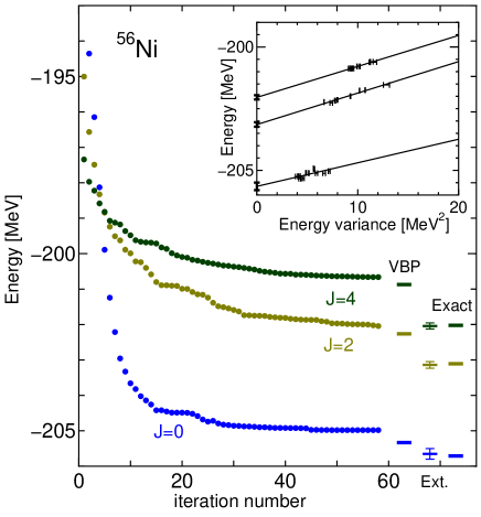
Figure 1: (Color online) Convergence patterns of energies with $J_{z}=$ 0, 2 and 4 states as functions of the iteration number for ⁵⁶Ni in the $pf$ shell with the GXPF1A Gxpf1a interaction. The $J$-projected energies (VBP) onto the converged states at $J_{z}=J$ space are shown with the extrapolated (Ext.) and exact (Exact) shell model energies. In the inset, extrapolations of energies with $J$ = 0, 2 and 4 as functions of energy variance are shown.

Next, we stochastically calculate the $J$-projected energy by carrying out a $J$-projection on the converged wave functions at $J_{z}=J$ space. We call this stochastic VBP (variation-before-projection). Note that the parameters of the wave function are optimized concerning number, parity, and $J_{z}$ projected energy. Here, we take $g_{K}=\delta_{KJ}$ for simplicity because we carry out the $J$-projection onto the wave functions optimized in the space with $J_{z}=J$. For $J=0$ state, after 1000 steps as a burn-in, a random walker moves 500000 steps in the $M$-scheme space. We evaluate the energy by 10 random walkers. The energy is -205.333 $\pm$ 0.004 MeV for ⁵⁶Ni. We show the $J$-projected energies for $J=0$, 2, and 4 with the label VBP in Fig. 1. The $J$-projection improves while there are still sizable differences between these VBP energies and exact shell model energies. In this formulation, we can stochastically evaluate electro-magnetic transition strengths with statistical errors. The calculated B(E2)’s with the VBP wave functions for $0\rightarrow 2$ and $2\rightarrow 4$ are 690 $\pm$ 8 and 134 $\pm$ 2 $e^{2}fm^{4}$, respectively. Here we use effective charges $e_{\pi}=1.5$ and $e_{\nu}=0.5$.

To overcome the variational limitation of the VMC, we introduce the energy variance extrapolation, which is a technique to estimate the exact energy from a series of approximated wave functions in a well-controlled way. This technique is based on a well-defined scaling property for energy eigenvalues. We define a difference $\delta E$ between energy eigenvalue $\langle H\rangle$ in a given subspace and exact energy eigenvalue $\langle H\rangle_{0}$, that is, $\delta E=\langle H\rangle-\langle H\rangle_{0},$ and an energy variance $\Delta E$ in the subspace is also defined as $\Delta E={\left\langle H^{2}\right\rangle-\left\langle H\right\rangle^{2}}.$ The difference $\delta E$ vanishes linearly or quadratically as a function of the energy variance $\Delta E$ exlanc . By this scaling property, we can estimate the exact shell-model energies as the limit of zero energy variance.

To apply this technique to the VMC, we introduce a truncation scheme in the form of a projection operator. In the case of the $pf$ shell, due to a relatively large gap of spherical single particle energy between the $f_{7/2}$ orbit and others $r$ ($f_{5/2}$, $p_{3/2}$ and $p_{1/2}$ orbits), particle-hole excitations across this shell gap form truncation spaces, $\oplus_{s\leq t}(f_{7/2})^{A-40-s}(r)^{s}$. The $P^{t}$ is a projection onto this truncation space and is added to the projection in Eqs.(3, 4). This projection operator is quite simply realized by the restriction of the summation in Eq.(8) and we can easily include this truncation scheme in the present VMC.

It is noteworthy that, in the Monte Carlo calculations, we find a fast computational method of the energy variance within the truncated space $t$ as

$$\left\langle H^{2}\right\rangle_{t}\sim\frac{W_{t}}{N_{0}}\sum_{i\in(t+2)}(E_{L}(m_{i}))^{2},$$ (35)

where $E_{L}$ is the local energy defined in Eq.(13), $N_{0}$ is a number of Monte Carlo sampler, and $W_{t}$ is a reweighing factor defined by the ratio between the number of random walkers within the $(t+2)$-space, that is, $N_{0}$, and one of random walkers within the $t$-space. By this sampling method, we can avoid the explicit calculation of four-body interaction for energy variance and its computation becomes possible.

In the inset of Fig. 1, energies of the VMC calculations with different truncation spaces and different initial conditions are plotted as functions of the energy variance, $\Delta E$. To the limit of zero energy variance, we can linearly extrapolate the energies with statistical errors obtained by the $\chi^{2}$ fitting. The extrapolated energies agree with the exact ones. In the same way, we can extrapolate the B(E2).

In conclusion, we have proposed a new variational Monte Carlo method with energy variance extrapolation for large-scale shell-model calculations. We have presented a formulation of wave function optimization based on the MCMC. In this method we can calculate approximated energy, other matrix elements, and electro-magnetic transitions for yrast states. Combining the VMC with energy variance extrapolation, we can estimate exact shell-model energies. This is an alternative extension of the VMC and is free from the sign-problem. By taking ⁵⁶Ni in the $pf$ shell, we have shown the feasibility of large-scale shell-model calculations. Note that the present calculations can be carried out with a single core of the common PC. For larger computations, parallel computation plays a significant role.

For further improvement of the present method, the stochastic VAP (variation-after-projection) concerning $J$-projection can improve accuracy of energy and energy variance to enhance the reliability of energy variance extrapolation. We are pursuing the stochastic VAP including its parallel computation as especially fitted to a state-of-the-art massive parallel computer, the results of which will be presented elsewhere.

For energy variance extrapolation, we introduced the particle-hole truncation scheme into the VMC while we can use the arbitrary basis-truncation scheme. The excitation-energy truncation scheme in the No-core Shell Model Nocore is also promising. We will investigate this direction in the future.

Finally, this study is motivated by a study of the Hubbard modelTahara . The present study sheds light onto a new way of projection in these stochastic calculations, an aspect of which may also be useful in applications of condensed matter physics.

One of the authors (N.S.) was supported by Grants-in-Aid for Young Scientists (20740127) from JSPS and the HPCI Strategic Program from MEXT.

Appendix

The Pfaffian is defined for a $2n\times 2n$ skew-symmetric matrix $A$ as

$$Pf(A)\displaystyle\equiv\frac{1}{2^{n}n!}\sum_{\sigma\in S_{2n}}{\rm sgn}(\sigma)\prod_{i=1}^{n}a_{\sigma(2i-1)\sigma(2i)}$$ (36)

where $\sigma$ is a permutation of $\{1,2,3,\cdots,2n\}$, ${\rm sgn}(\sigma)$ is its sign, $S_{2n}$ is symmetry group and $a$’s are matrix elements of $A$. An efficient computation of the Pfaffian can be seen e.g. in Ref.phaff .

References

- (1) E. Caurier, F. Nowacki, A. Poves, K. Sieja, Phys, Rev. C 82 064304 (2010).
- (2) N. Shimizu, Y. Utsuno, T. Mizusaki, T. Otsuka, T. Abe, and M. Honma, AIP Conf. Proc. 1355, in press.
- (3) S. E. Koonin, D. J. Dean, and K. Langanke, Phys. Rep. 278, 1 (1997).
- (4) J. Dukelsky, S. Pittel, Phys. Rev. C 63 061303 (2001); B. Thakur, S. Pittel, N. Sandulescu, Phys. Rev. C 78, 041303 (2008).
- (5) A. Petrovici, Nucl. Phys. A 704, 144c (2002).
- (6) G. Hagen, D. J. Dean, M. Hjorth-Jensen, T. Papenbrock, Phys. Lett. B 656 169-173 (2007).
- (7) M. Honma, T. Mizusaki, and T. Otsuka, Phys. Rev. Lett. 75, 1284 (1995).
- (8) T. Otsuka, M. Honma, T. Mizusaki, N. Shimizu, and Y. Utsuno, Prog. Part. Nucl. Phys. 47, 319 (2001).
- (9) T. Mizusaki and M. Imada, Phys. Rev. C 65, 064319 (2002); ibid. 67, 041301 (2003).
- (10) T. Papenbrock, A. Juodagalvis, D. J. Dean, Phys. Rev. C69 (2004) 024312.
- (11) N. Shimizu, Y. Utsuno, T. Mizusaki, T. Otsuka, T. Abe, M. Honma, Phys. Rev. C 82 061305 (2010).
- (12) M. Imada and T. Kashima, J. Phys. Soc. Jpn. 69 2723 (2000).
- (13) S. Sorella, Phys. Rev. B64, 024512 (2001).
- (14) S. Sorella, Phys. Rev. Lett. 80 4558 (1998).
- (15) D. Tahara and M. Imada, J. Phys. Soc. Jpn. 77 114701 (2008).
- (16) P. Ring and P. Schuck, The Nuclear Many-Body Problem, (Springer-Verlag, New York, Heidelberg, Berlin, 1980).
- (17) M. Honma, et al., Eur. Phys. J. A 25, Suppl. 1, 499 (2005).
- (18) H. Zhan, A. Nogga, B. R. Barrett, J. P. Vary, and P. Navratil, Phys. Rev. C69, 034302 (2004).
- (19) W. Wimmer, arXiv:cond-mat/1102.3440 (2011).