Expected constraints on the Galactic magnetic field using PLANCK data

Abstract

Aims. We explore in this paper the ability to constrain the Galactic magnetic field intensity and spatial distribution with the incoming data from the Planck satellite experiment.

Methods. We perform realistic simulations of the Planck observations at the polarized frequency bands from 30 to 353 GHz for two all–sky surveys as expected for the nominal mission. These simulations include CMB, synchrotron and thermal dust Galactic emissions and instrumental noise. (Note that systematic effects are not considered in this paper). For the synchrotron and thermal dust Galactic emissions we use a coherent 3D model of the Galaxy describing its mater density and the magnetic field direction and intensity. We first simulate the synchrotron and dust emissions at 408 MHz and 545 GHz, respectively, and then we extrapolate them to the Planck frequency bands.

Results. We perform a likelihood analysis to compare the simulated data to a set of models obtained by varying the pitch angle of the regular magnetic field spatial distribution, the relative amplitude of the turbulent magnetic field, the radial scale of the electron and dust grain distributions, and the extrapolation spectral indices for the synchrotron and thermal dust emissions. We are able to set tight constraints on all the parameters considered. We have also found that the observed spatial variations of the synchrotron and thermal dust spectral indices should not affect our ability to recover the other parameters of the model.

Conclusions. From this, we conclude that the Planck satellite experiment can precisely measure the main properties of the Galactic magnetic field. An accurate reconstruction of the matter distribution would require on the one hand an improved modelling of the ISM and on the other hand to use extra data sets like rotation measurements of pulsars.

1 Introduction

The Planck satellite (Planck-Collaboration, 2011a; Tauber et al., 2010), currently in flight, will provide measurements of the CMB anisotropies both in temperature and polarization over the full-sky at unprecedented accuracy. It covers a large range of frequencies from 30 to 857 GHz and therefore is able to give a measurement of the foreground emissions. Planck makes observations of the sky with a combined sensitivity of $\Delta T/T_{CMB}\sim 2\times 10^{-6}$ (Planck-Collaboration, 2005) and an angular resolution from 33 to 5 arcmin (Planck-Collaboration, 2005). In particular, because of its 7 polarized channels it will for the first time allow the simultaneous precise measurement of the main sources of polarized Galactic emissions: synchrotron and thermal dust.

Using the Wmap (Wilkinson Microwave Anisotropy Probe), Page et al. (2007) have shown that the synchrotron emission is highly polarized, up to 70% between 23 and 94 GHz. Furthermore, Benoît et al. (2004); Ponthieu et al. (2005) have observed significantly polarized thermal dust emission, up to 15 % in the 353 GHz Archeops channel. The free-free emission is not intrinsically polarized and the anomalous dust-correlated emission is weakly polarized at $3^{+1.3}_{-1.9}$ (Battistelli et al., 2006). At the Planck frequency bands the polarized contribution from compact and point sources is expected to be weak for both radio (Nolta, 2009) and dusty (Désert et al., 1990) sources. The frequency and spatial distributions of the polarized diffuse Galactic emissions are not currently well known and the only available informations come from microwave and submillimeter observations.

The Galactic synchrotron emission originate from relativistic electrons spiraling along magnetic field lines. The direction of polarization is orthogonal both to the line-of-sight and to the field lines.

The synchrotron emission contributes principally to diffuse emission at both radio and microwave observation frequencies. Its spectral energy distribution (SED) is not known with accuracy however it is assumed to be well reproduced by a power law in antenna temperature $T_{\nu}\alpha\nu^{\beta_{s}}$ with a spectral index ranging form -2.7 to -3.4 (Lawson et al., 1987; Reich & Reich, 1988; Reich et al., 2004; Kogut et al., 2007; Gold et al., 2009; Fauvet et al., 2010) . The Galactic synchrotron emission has been well traced by the Leiden survey between 408 MHz and 1.4 GHz (Brouw & Spoelstra, 1976; Wolleben et al., 2006), the Parkes survey at 2.4 GHz (Duncan et al., 1999) and the MGLS ( Medium Galactic Latitude Survey) at 1.4 GHz (Uyaniker et al., 1999). At the microwave frequencies it has been mapped by Wmap, see e.g. Hinshaw et al. (2009); Page et al. (2007).

Thermal dust emission arises from dust grains in the interstellar medium (ISM) with typical sizes $\simeq$ 0.25 $\mu$m that are heated by stellar radiation (Désert et al., 1990). This emission can be partially polarized as prolate dust grains align with their long axis perpendicular to the magnetic field (Davis & Greenstein, 1951). The dust emission efficiency is greatest along the long axis, leading to partial linear polarization perpendicular to the magnetic field. The fractional polarization depends on the grain size distribution and is typically a few percent at millimeter wavelengths (Hildebrand et al., 1999; Vaillancourt, 2002; Fauvet et al., 2010). The thermal dust emission in intensity has already been well measured by Iras form 5 to 100 $\mu$m (Neugebauer et al., 1984) and COBE/FIRAS which provided the first polarized observation at high frequencies. Currently, Planck HFI (Planck-HFI-Core-Team, 2010) is measuring this emission in intensity (Planck-Collaboration, 2011b, c, d, e).

Based on the physical characteristics of the synchrotron emission, Page et al. (2007) proposed a 3D model of the Galaxy including the distribution of relativistic electrons and the spatial distribution of the Galactic magnetic field. Independently, Han et al. (2004, 2006) used a 3D model of the free electrons density in the Galaxy (Cordes & Lazio, 2002) and a model of the Galactic magnetic field including regular and turbulent components to explain the observed rotation measurements toward known pulsars. Based on these works Sun et al. (2008) performed a combined analysis of the rotation measurement of pulsars and of the polarized Wmap data. This work has been extended by Jaffe et al. (2010) to study the Galactic plane and Jansson et al. (2009) for the full sky. Recently Fauvet et al. (2010) proposed for the first time a coherent model of the synchrotron and thermal dust Galactic emissions using the Wmap and Archeops data. In addition to the above, many other related models and analyses can be found in the literature.

We propose in this paper a method to study and constrain the synchrotron and thermal dust polarized emissions using the Planck satellite observations that are currently underway. Using realistic simulations of the Planck polarized data we forecast the expected constraints on a 3D model of the Galactic magnetic field and the Galactic matter distribution. This paper is structured as follows: in Section 2.1 we describe the models we used for the polarized components of the Galactic diffuse emissions and in Section 3 we present the simulations of data used in this analysis. In Section 4 we describe our method to constrain these Galactic foreground emission models and we discuss the results in Section 5. Conclusions are presented in Section 6.

2 Models of polarized Galactic emissions

A realistic model of synchrotron and thermal dust emissions can be constructed from a 3D description of the Galaxy including the matter distribution and the magnetic field structure. Following Fauvet et al. (2010), we calculate the Stokes parameters I, Q and U of the emerging polarized Galactic emissions along the line-of-sight n.
For the synchrotron emission, in galactocentric cylindrical coordinates $(r,\phi,z)$ we use the following model (Fauvet et al., 2010):

$$I_{\mathrm{sync}}(\mathrm{{\bf n}}) = I_{\mathrm{Has/ff}}(\mathrm{{\bf n}})\left(\frac{\nu_{s}}{0.408}\right)^{\beta_{s}},$$

$$Q_{\mathrm{sync}}(\mathrm{{\bf n}}) = I_{\mathrm{Has/ff}}(\mathrm{{\bf n}})\left(\frac{\nu_{s}}{0.408}\right)^{\beta_{s}}$$

$$.\frac{\int\cos(2\gamma({\bf n},s))p_{s}\left(B_{l}^{2}({\bf n},s)+B_{t}^{2}({\bf n},s)\right)\mathrm{n}_{\mathrm{CRE}}(r,z)ds}{\int\left(B_{l}^{2}({\bf n},z)+B_{t}^{2}({\bf n},s)\right)\mathrm{n}_{\mathrm{CRE}}(r,z)ds},$$

$$U_{\mathrm{sync}}(\mathrm{{\bf n}}) = I_{\mathrm{Has/ff}}(\mathrm{{\bf n}})\left(\frac{\nu_{s}}{0.408}\right)^{\beta_{s}}$$

$$.\frac{\int\sin(2\gamma({\bf n},s))p_{s}\left(B_{l}^{2}({\bf n},s)+B_{t}^{2}({\bf n},s)\right)\mathrm{n}_{\mathrm{CRE}}(r,z)ds}{\int\left(B_{l}^{2}({\bf n},s)+B_{t}^{2}({\bf n},s)\right)\mathrm{n}_{\mathrm{CRE}}(r,z)ds},$$

where $B_{n}(\mathrm{{\bf n}},s)$ is the magnetic component along the line-of-sight n, and $B_{l}(\mathrm{{\bf n}},s)$ and $B_{t}(\mathrm{{\bf n}},s)$ the magnetic field components on a plane perpendicular to the line-of-sight. The polarization fraction $p_{s}$ is set to 75% (Rybicki & Lightman, 1979). The polarization angle $\gamma(\mathrm{{\bf n}},s)$ is given by :

$$\centering\gamma(\mathrm{{\bf n}},s)=\frac{1}{2}\arctan\left(\frac{2B_{l}(\mathrm{{\bf n}},s)\cdot B_{t}(\mathrm{{\bf n}},s)}{B^{2}_{l}(\mathrm{{\bf n}},s)-B^{2}_{t}(\mathrm{{\bf n}},s)}\right)\@add@centering$$ (1)

The distribution of relativistic electrons, $\mathrm{n}_{\mathrm{CRE}}$, is described in details in section 2.1.1. $I_{Has/ff}$ is a template temperature map obtained from the 408 MHz all-sky continuum survey (Haslam et al., 1982). This map is also included bremsstrahlung (free-free) emission. To substract this component we used the Wmap K-band free-free foreground map generated from the maximum entropy method (MEM) (Hinshaw et al., 2007; Bennett et al., 2003). Note that this template is not necessarily realistic; Alves et al. (2010) have shown with radio recombination lines that in at least one region in the Galactic plane, this model appears to overestimate the amount of free-free. However, that will not have any impact in the following analysis because we used the same template in the simulated data and in the fitted models and the uncertainty at 408 MHz is very small compared to the synchrotron amplitude. The free-free map is then extrapolated to 408 MHz assuming a power law dependance as in Dickinson et al. (2003). The spectral index $\beta_{s}$ used to extrapolate maps at various frequencies is a free parameter of the model and will be discussed later.

For the thermal dust emission we used the following model (Fauvet et al., 2010):

$$\centering I_{\mathrm{dust}}(\mathrm{{\bf n}})\@add@centering = \mathrm{I}_{\mathrm{fds}}(\mathrm{{\bf n}})\left(\frac{\nu_{d}}{353}\right)^{\beta_{d}},$$

$$Q_{\mathrm{dust}}(\mathrm{{\bf n}}) = \mathrm{I}_{\mathrm{fds}}(\mathrm{{\bf n}})\left(\frac{\nu_{d}}{353}\right)^{\beta_{d}}$$

$$.\frac{\int\cos(2\gamma(\mathrm{{\bf n}},s))\sin^{2}(\alpha)f_{\mathrm{norm}}p_{d}\mathrm{n}_{\mathrm{dust}}(r,z)ds}{\int\mathrm{n}_{\mathrm{dust}}(r,z)ds},$$

$$U_{\mathrm{dust}}(\mathrm{{\bf n}}) = \mathrm{I}_{\mathrm{fds}}(\mathrm{{\bf n}})\left(\frac{\nu_{d}}{353}\right)^{\beta_{d}}$$

$$.\frac{\int\sin(2\gamma(\mathrm{{\bf n}},s))\sin^{2}(\alpha)f_{\mathrm{norm}}p_{d}\mathrm{n}_{\mathrm{dust}}(r,z)ds}{\int\mathrm{n}_{\mathrm{dust}}(r,z)ds},$$

where the dust polarization fraction $p_{d}$ is set to 10 % (Ponthieu et al., 2005), and $\mathrm{n}_{\mathrm{dust}}(r,z)$ is the dust grain distribution discussed in section 2.1.1. The $sin^{2}(\alpha)$ term accounts for geometrical supression and $f_{norm}$ is an empirical factor which accounts for the misalignment between dust grains and the magnetic field lines (see Fauvet et al. (2010) for details). The reference map, $\mathrm{I}_{\mathrm{fds}}$, is the Finkbeiner et al. (1999) model 8 prediction based on the Iras data (Neugebauer et al., 1984) and on the COBE/DIRBE data. The spectral index $\beta_{d}$ used to extrapolate maps at various frequencies is a free parameter of the model. This template seems to be a good representation of the Archeops data at 353 GHz as discussed in Macías-Pérez et al. (2007). Notice that for the polarized Planck frequencies, we are in the Rayleigh-Jeans domain and therefore, a power-law approximation for the dust intensity can be used.

2.1 3D model of the Galaxy

We describe here our 3D model of the Galaxy.

2.1.1 Matter density

We consider an exponential distribution of relativistic electrons $\mathrm{n}_{\mathrm{CRE}}$ on the Galactic disk motivated by Drimmel & Spergel (2001):

$$\centering\mathrm{n}_{\mathrm{CRE}}(r,z)=n_{0,e}\cdot\frac{e^{-\frac{r}{\mathrm{n}_{\mathrm{CRE},r}}}}{\cosh^{2}(z/\mathrm{n}_{\mathrm{CRE},h})}\@add@centering$$ (2)

where $\mathrm{n}_{\mathrm{CRE,r}}$ is the scale radius of the distribution and is a free parameter of the model. The vertical scale height, $\mathrm{n}_{\mathrm{CRE,h}}$, is set to 1 kpc. The value of $n_{0,e}$ is set to $6.4\times 10^{-6}$cm^-3, following Sun et al. (2008).
The distribution of dust grains $\mathrm{n}_{\mathrm{dust}}$ is described in the same way that of relativistic electrons with:

$$\centering\mathrm{n}_{\mathrm{dust}}(r,z)=n_{0,d}\cdot\frac{e^{-\frac{r}{\mathrm{n}_{d,r}}}}{\cosh^{2}(z/\mathrm{n}_{d,h})},\@add@centering$$ (3)

where the scale radius $n_{d,r}(r,z)$ is also a free parameter of the model (see Fauvet et al. (2010) for more details). The vertical scale height, $\mathrm{n}_{d,r}$, is set to 1 kpc.

2.1.2 Galactic magnetic field model

The Galactic magnetic field model is composed of two parts: a regular component and a turbulent component such that $\@vec{B}=\@vec{B}_{reg}+\@vec{B}_{turb}$ (bold letters indicate vectorial quantities). We include only the isotropic part of the turbulent magnetic field and no anisotropic/ordered component (see Jaffe et al. (2010)). As in Fauvet et al. (2010), our regular component is then equivalent to the sum of what Jaffe et al. (2010) call the coherent and ordered fields. For this analysis of synchrotron and dust emission only, the distinction is irrelevant. For the regular component we consider a Modified Logarithmic Spiral model (MLS), presented in Fauvet et al. (2010) and based on the Wmap model (Page et al., 2007). In cylindrical coordinates $(r,\phi,z)$ it reads :

$$\centering\mathbf{\@vec{B}_{reg}}(\mathbf{r})\@add@centering = B(\mathbf{r})[\cos(\phi+\beta)\ln\left(\frac{r}{r_{0}}\right)\sin(p)\cos(\chi(r))\cdot\mathbf{u_{r}}$$ (4)

$$-\cos(\phi+\beta)\ln\left(\frac{r}{r_{0}}\right)\cos(p)\cos(\chi(r))\cdot\mathbf{u_{\phi}}$$

$$+sin(\chi(r))\cdot\mathbf{u_{z}}],$$

where the pitch angle, $p$, is a free parameter of the model and $\beta=1/\tan(p)$. The scale radius $r_{0}$ is set to 7.1 kpc and $\chi(r)=\chi_{0}(r)(z/z_{0})$ is the vertical scale height, with $\chi_{0}=22.4$ degrees and $z_{0}=1$kpc. The intensity of the regular field is fixed using pulsar Faraday rotation measurements by Han et al. (2006):

$$B(r)=B_{0}\ e^{-\frac{r-R_{\odot}}{R_{B}}}$$ (5)

where the large-scale field intensity at the Sun position is $B_{0}=2.1\pm 0.3\mu G$ and $R_{B}=8.5\pm 4.7kpc$. The distance between the Sun and the Galactic center, $R_{\odot}$ is set to 8 kpc (Eisenhauer et al. (2003); Reid & Brunthaler (2005)).

2.1.3 Turbulent component

In addition to the large-scale Galactic magnetic field, Faraday rotation measurements on pulsars in our vicinity have revealed a turbulent component (Lyne & Smith, 1989; Han et al., 2004) with an amplitude estimated to be of the same order of magnitude as that of the regular one (Han et al., 2006).

The turbulent magnetic field is assumed to be a 3D anisotropic gaussian random vectorial field and it is fully determined by a spherically symmetric power spectrum in the Fourier domain. Indeed, the magnetic energy $E_{B}(k)$ associated with the turbulent component can be described by a power spectrum of the form (Han et al. (2004, 2006))

$$\centering E_{B}(k)=C\left(\frac{k}{k_{0}}\right)^{\alpha}\@add@centering$$ (6)

where $\alpha=-0.37$ and $C=(6.8\pm 0.3)\cdot 10^{-13}\,\mathrm{erg\,cm^{-3}\,kpc}$. More complex models of this anisotropic turbulent component have been proposed by (Higdon, 1984; Cho et al., 2002) and Cho & Lazarian (2010) but they are beyond the scope of this paper. Note also that we do not consider here the so-called ordered turbulent component of the Galactic magnetic field as discussed in Jaffe et al. (2010).

3 Simulated data

We have performed simulations of the Planck polarized observations. We considered all the polarized channels for the LFI (Bersanelli et al., 2010; Mandolesi et al., 2010; Menella et al., 2011) and HFI (Lamarre et al., 2010; Planck-HFI-Core-Team, 2010) instruments at 30, 44, 70, 100, 143, 217 and 353 GHz for two full-sky surveys (14 months). We did not use the total intensity maps in this analysis. For this set of simulations we generated full-sky maps in the HEALPix pixelisation scheme (Górski et al., 2005) at $N_{side}=128$. The input templates are simply degraded to that resolution using the HEALPix tools.
At a given observation frequency, $\nu$, we consider that the polarized observations ($X^{\nu}$) are the sum of the synchrotron ($X^{\nu}_{\mathrm{sync}}$) and the thermal dust emissions ($X^{\nu}_{\mathrm{dust}}$), where $X$ is the Q or U Stokes parameter. We also add a CMB contribution ($X^{\nu}_{CMB}$) and noise ($X^{\nu}_{N}$) so that can finally write: $X^{\nu}=X^{\nu}_{\mathrm{dust}}+X^{\nu}_{\mathrm{sync}}+X^{\nu}_{N}+X^{\nu}_{\mathrm{CMB}}$

3.1 Polarized Galactic emission components

The polarized Galactic emissions are simulated using the 3D model described in Section 2.1. The parameters of the 3D model of the Galaxy have been taken from Fauvet et al. (2010) by comparison with the available Archeops (Benoît et al., 2004) and Wmap 5-years data (Hinshaw et al., 2009). The pitch angle is set to -30 degrees and the radial widths of the distributions of dust grains $n_{d,r}$ and ultrarelativist electrons $n_{CRE,r}$ are set to 3 kpc. We computed simulated data using a model of Galactic magnetic field without (Simu I) or with a turbulent component (Simu II). In the second case we set the amplitude of the turbulent component to $A_{turb}=0.25\times B(r)$. The simulations are extrapolated to each of the Planck frequencies assuming constant spectral indices in frequency and using two different configurations, either spatially constant (Simu Cst) or variable (Simu Var) accross the sky. We have produced at least 10 simulations for each of the different configurations.

In the Simu Cst case we set the value of the synchrotron spectral index to $\beta_{s}=-3.0$. Concerning the thermal dust emission we test both upper and lower expected limits of the spectral index. We tested 1.4 as a lower limit, obtained by comparison of a grey body law model to the Archeops and Iris data in the galactic plane. The upper limit tested is 2, following results obtained at high latitude by Boulanger et al. (1996) using the Firas and Dirbe data.

For the Simu Var case, the maps of $\beta_{s}$ and $\beta_{d}$ are built in the following way. For the synchrotron emission we used the map generated using a MCMC fit by Kogut et al. (2007) at 23 GHz applying some corrections. We cut all pixels where $\beta_{s}<-3.5$ and $\beta_{s}>-2.8$, following the results in Page et al. (2007); Sun et al. (2008); Fauvet et al. (2010), and assumed for those pixels $\beta_{s}=-3.0+0.1*n$, where $n$ is a gaussian random normal distribution. Note that $\beta_{s}$ is the typical average value found in the literature. It is also important to clarify that this spectral index map was not derived from the MEM analysis of the Wmap data. However, it can be used as a fair representation of the variability of the spectral index. The resulting synchrotron spectral index map is shown in the left panel of Figure 1.
To simulate the spatial variations of the spectral index of the thermal dust emission we assumed a random gaussian distribution with a mean value of $\beta_{d,mean}=1.4$ or $\beta_{d,mean}=2.0$ and a standard deviation of 0.3. The right panel of Figure 1 shows the resulting thermal dust spectral index map. Table 1 summarizes the resulting types of simulations that we carried out.

Table 1: Summary of the different types of simulations considered in this paper.

Simulation	$\beta_{s,d}$	$A_{turb}$
Simu 1	constant	$0.0\times B_{reg}$
	variable	$0.0\times B_{reg}$
Simu 2	constant	$0.25\times B_{reg}$
	variable	$0.25\times B_{reg}$

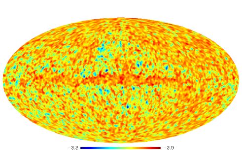
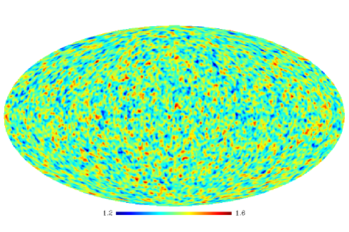
Figure 1: Spatial variations of the spectral indices for the simulated synchrotron (left) and thermal dust Galactic polarized emissions (right).

3.2 CMB emission

We produced maps at $N_{side}=128$ of the expected CMB signal at all the Planck frequencies. We used CAMB (Lewis et al., 2000) to compute the CMB temperature and polarization angular power spectra for the Wmap $\Lambda CDM$ best fit model as estimated by (Komatsu et al., 2009). We also took into account gravitational lensing effects and assumed a tensor-scalar ratio, $r$, of 0.1 (Efstathiou et al., 2009).

3.3 Noise

Planck noise maps for each of the frequency channels were computed using the mean sensitivity per pixel given in Table 2. We assumed isotropic random gaussian noise accross the sky. This is not actually the case for the real Planck scanning strategy (Dupac, 2005). However this should not have any impact on the presented results as we are mostly signal dominated.

Table 2: Average 1$\sigma$ sensitivity per pixel (a square whose side is the FWHM extent of the beam) in thermodynamic temperature units, achievable after 2 full sky surveys (14 months) by Planck. (Planck-Collaboration, 2005)

Center frequency [GHz]	30	44	70	100	143	217	353
($\Delta T/T$) polarization [$\mu K/K$]	2.8	3.9	6.7	4.0	4.2	9.8	29.8
Angular resolution [arcmin FWHM]	33	24	14	10	7	5	5

4 Method

Table 3: Parameters of the 3D Galactic polarized diffuse emission models.

Parameters	Range	Binning
$p$ (deg)	$[-80.0,80.0]$	$10.0$
$A_{turb}$	$[0,2.5]*B_{reg}$	$0.125$
$n_{CRE,r}$ (kpc)	$[1.0,20.0]$	$1$
$n_{d,r}$ (kpc)	$[1.0,20.0]$	$1$
$\beta_{s}$	$[-4.3,-2.4]$	$0.1$
$\beta_{d}$	$[2.0,4.0]$	$0.1$

Following Fauvet et al. (2010), in order to compare the models of Galactic polarized emissions to the Planck data simulations we computed Galactic profiles in polarization using the set of latitude bands (in degrees) $[0,30]$, $[30,60]$, $[60,90]$, $[90,120]$,$[120,180]$, $[180,270]$, $[270,330]$, $[330,360]$. Note that the intensity profiles are not used in this paper as the intensity maps were constructed using fixed templates.

Galactic latitude profiles for the diffuse Galactic polarized emission models were computed for a grid of models obtained by varying the pitch angle, $p$, the turbulent component amplitude, $A_{turb}$, the radial scale for the distribution of electrons, $n_{CRE,r}$ and of dust grains $n_{d,r}$, and the spectral indices $\beta_{s}$ and $\beta_{d}$. The latter were assumed to be spatially constant accross the sky. All the others parameters were set to the values proposed in section 3.1.

We compared the simulated data sets to the Galactic emission models using a likelihood analysis where the log-likelihood function is given by:

$$-log\mathcal{L}=\\ \frac{\sum_{\nu=0}^{nfreq-1}\sum_{i=0}^{nlon-1}\sum_{n=0}^{nlat-1}(S^{\nu}_{i,X}(n)-M^{\nu}_{i,X}(n))^{2}}{\sigma^{\nu}_{i,X}(n)^{2}+\sigma^{\nu,turb}_{i,X}(n)^{2}}$$

where the $X$ are the Stokes parameters $Q$ and $U$, and $i$ and $n$ index the longitude bands and the latitude bins, respectively. $S^{\nu}_{i,X}(n)$ and $M^{\nu}_{i,X}(n)$ are the set of simulations and models respectively for the polarization state $X$, $i$ longitude band and $n$ longitude bin. The term $\sigma^{\nu}_{i,X}(n)^{2}$ is the error associated to $S^{\nu}_{i,X}(n)$ computed from the standard deviation of the data samples in each of the latitude bins. Note that it accounts both for the noise and signal dispersion within the bin. The term $\sigma^{\nu,turb}_{i,X}(n)$ accounts for the additional variance due to the turbulent component of the magnetic field. Indeed, as the magnetic field is considered to be a random distribution, we need to take into account in the likelihood function an extra correlation matrix. We approximated this matrix to a diagonal one. We used 10 simulations of the Galactic turbulent contribution at each Planck frequency band to estimate $\sigma^{\nu,turb}_{i,X}(n)$. Note that the latter term is proportional to $A_{turb}$ and also to the extrapolation term, $(\frac{\nu}{\nu_{ref}})^{\beta}$, both for the synchrotron and thermal dust components. This may introduce a small bias in the A_turb, $\beta_{s}$ and $\beta_{d}$ parameters. Increased turbulence can be balanced by a steeper spectral index and therefore it is possible to lower the resulting $\chi^{2}$ for some parameter combinations. We will see, however, that the impact of this bias on the results remains small.

Table 4: Best-fit parameters for the Galactic polarized emission models in the case of $\beta_{d}=1.4$ in the simulated data. In the case of simulations with turbulence, Simu II, we give for each parameter the variance among the set of simulation results.

Simulation	Simu I		Simu II
$\beta_{simu}$	Cst	Var	Cst	Var
$A_{turb}$	$<0.1$	$<0.1$	$0.25^{+0.2}_{-0.1}$	$0.25^{+0.2}_{-0.1}$
$p(deg)$	$-30^{+4}_{-6}$	$-30^{+4}_{-6}$	$-30^{+8}_{-14}$ (5)	$-30^{+8}_{-14}$ (5)
$n_{CRE,r}$	$3^{+1.5}_{-1}$	$3^{+1.5}_{-1}$	$12^{+6}_{-8}$ (4.5)	$12^{+6}_{-8}$ (4.5)
$n_{d,r}$	$3^{+10}_{-1}$	$3^{+10}_{-1}$	$<16$ (5.1)	$12{+6}_{-8}$ (4.5)
$\beta_{s}$	$-3.0^{+0.05}_{-0.1}$	$-3.0^{+0.05}_{-0.1}$	$-3.1^{+0.1}_{-0.7}$ ( $<$ 0.05)	$-3.1^{+0.1}_{-0.7}$ ( $<$ 0.05)
$\beta_{d}$	$1.4\pm 0.1$	$1.4^{+0.2}_{-0.4}$	$1.5^{+0.5}_{-0.3}$ (0.05)	$1.5^{+0.5}_{-0.3}$ (0.05)

Table 5: Best-fit parameters for the Galactic polarized emission models in the case of $\beta_{d}=2.0$ in the simulated data. In the case of simulations with turbulence, Simu II, we give for each parameter the variance among the set of simulation results.

Simulation	Simu I		Simu II
$\beta_{simu}$	Cst	Var	Cst	Var
$A_{turb}$	$<0.1$	$<0.1$	$0.35^{+0.2}_{-0.1}$ (0.06)	$0.35^{+0.2}_{-0.1}$(0.06)
$p(deg)$	$-30^{+4}_{-6}$	$-30^{+4}_{-6}$	$-30^{+12}_{-14}$ (7.5)	$-30^{+12}_{-14}$ (7.5)
$n_{CRE,r}$	$3^{+1.5}_{-1}$	$3^{+1.5}_{-1}$	$12^{+6}_{-8}$ (4.1)	$12^{+6}_{-8}$ (4.1)
$n_{d,r}$	$3^{+10}_{-1}$	$3^{+10}_{-1}$	$<16$ (2)	$12^{+6}_{-8}$ (2)
$\beta_{s}$	$-3.0^{+0.05}_{-0.1}$	$-3.0^{+0.05}_{-0.1}$	$-3.1^{+0.1}_{-0.7}$ ( 0.05)	$-3.1^{+0.1}_{-0.7}$ (0.05)
$\beta_{d}$	$2.0\pm 0.1$	$2.0^{+0.2}_{-0.4}$	$2.2^{+0.5}_{-0.3}$ (0.05)	$2.3^{+0.5}_{-0.3}$ (0.05)

5 Results and discussion

The expected constraints on the parameters of the polarized Galactic emission models using the simulated Planck data are given in Tables 4 and 5 for the various sets of simulations considered.

5.1 Simu I

The constraints obtained for the Simu I cases are presented in the first line of Tables 4 and 5. The associated marginalized likelihood in 1 and 2D are shown in Figure 2 for the parameters $A_{turb}$, $p$, $n_{CRE,r}$, $n_{d,r}$, $\beta_{s}$ and $\beta_{d}$, and we present the 1, 2 and 3$\sigma$ confidence level contours. We can see that there is no correlation between the parameters. We are able to tightly constrain all the parameters of the Galactic emission models. Furthermore, we can see that the best fit values coincide with the parameters used in the input simulations. Therefore, there is no indication of bias in the method. We can see that spatial variations of the spectral indices do not disturb the constraints on the parameters. Indeed the expected constraints on all the parameters of the models, including the values of spectral indices, are unchanged. This could be explained by the fact that we use a Galactic profile based comparison which is not very sensitive to pixel-to-pixel variations but rather to global features. The constraint on the dust grain density parameter is weaker than that for the relativistic electrons density. This is probably due to the fact that the synchrotron is dominant at the Planck frequencies.

5.2 Simu II

The results concerning the Simu II cases, i.e. those including a turbulent component, are summarized in the lines 3 and 4 of Tables 4 and 5. The marginalized likelihoods in 1 and 2D for the parameters $A_{turb}$, $p$, $n_{CRE,r}$, $n_{d,r}$, $\beta_{s}$ and $\beta_{d}$ are shown in figure 3 on which we present the 1, 2 and 3$\sigma$ confidence level contours. We observe that there is no correlation between parameters, however, the constraints on the different parameters are weaker by a factor of 2 or more compared to the Simu I case. We observe a small bias on the best-fit values of the two spectral indices, but it is within the 1$\sigma$ error bars; it is related to the additional noise-like term added to the likelihood calculation by the turbulent component of the magnetic field. Furthermore, the radial scales $n_{CRE,r}$ and $n_{d,r}$ are not constrained. A degeneracy between the matter distribution and the other parameters of the models is induced by the method of construction but is not visible in the Figure 3. Nevertheless, an upper limit can be set. Because the millimeter and submillimeter data are not very sensitive to changes in those parameters, as was discussed in Fauvet et al. (2010), only an upper limit can be determined.

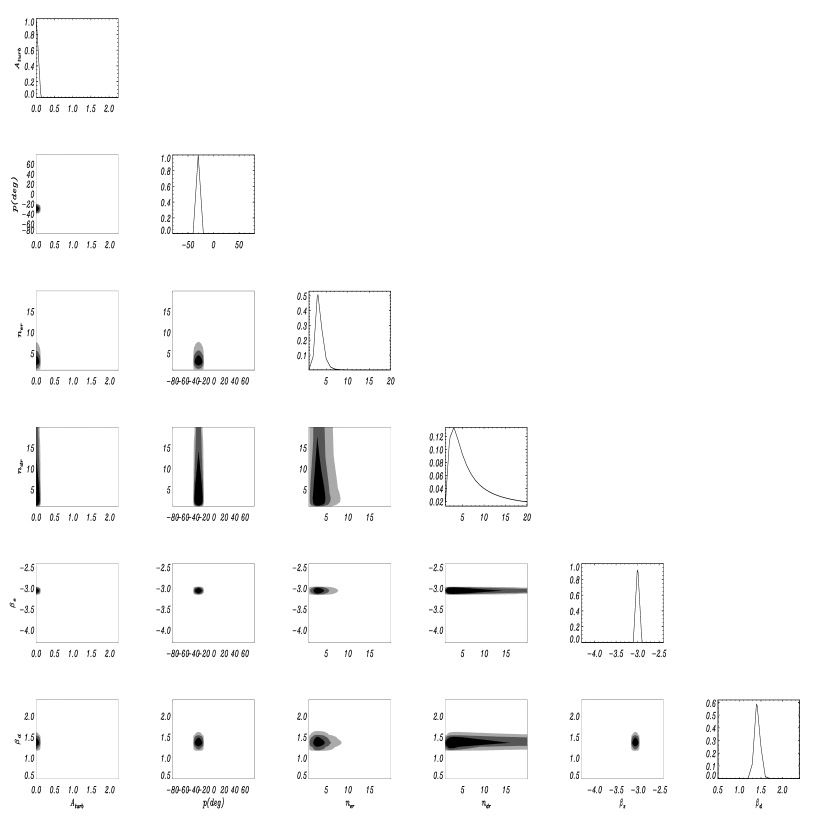
Figure 2: Marginalised likelihood in 1 and 2D for the parameters $A_{turb}$ and $p$, $n_{CRE,r}$ , $n_{d,r}$, $\beta_{s}$ and $\beta_{d}$ for the (Simu I Cst) case and we present the 1 (68.8%), 2 (95.4%) and 3$\sigma$ (98%) confidence level contours. The values of the parameters included in the simulated data are set to $A_{turb}$=0, $p=-30^{\circ}$, $n_{CRE,r}=n_{d,r}=3$kpc, $\beta_{s}=-3.0$, $\beta_{d}=1.4$ respectively.

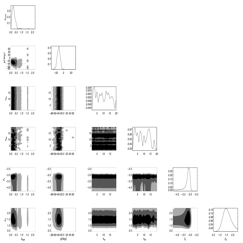
Figure 3: Marginalised likelihood in 1 and 2D for the parameters $A_{turb}$ and $p$, $n_{CRE,r}$ , $n_{d,r}$, $\beta_{s}$ and $\beta_{d}$ for the (Simu II Var) case and we present the 1 (68.8%), 2 (95.4%) and 3$\sigma$ (98%) confidence level contours. The values of the parameters included in the simulated data are set to $A_{turb}$=0, $p=-30^{\circ}$, $n_{CRE,r}=n_{d,r}=3$kpc, $\beta_{s}=-3.0$, $\beta_{d}=1.4$ respectively.

6 Summary and Conclusions

We proposed a method to estimate the expected constraints on the Galactic diffuse polarized emissions and the Galactic magnetic field at large scales using the Planck data. With this aim, we computed realistic simulations of the Planck data at the polarized frequency bands for two all-sky surveys. These simulations include CMB, synchrotron and thermal dust emissions and instrumental noise. For the synchrotron and thermal dust Galactic emissions we used a coherent 3D model of the Galaxy describing the magnetic field direction and intensity and the distribution of matter. The relativistic electron and dust grain densities were modeled using exponential distributions in galactocentric coordinates. For the Galactic magnetic field we considered the Modified Logarithmic Spiral model discussed in Fauvet et al. (2010).

We performed a likelihood analysis to compare the simulated Planck data to a set of models obtained by varying the pitch angle of the regular magnetic field spatial distribution, the relative amplitude of the turbulent magnetic field, the radial scale of the electron and dust grain distributions as well as the extrapolation indices of the synchrotron and thermal dust emissions. We are able to set accurate constraints on most of the parameters considered. We have also found that the observed spatial variations of the synchrotron and thermal dust spectral indices should not affect our ability to recover the other parameters of the model. The presence of a turbulent component of the Galactic magnetic field decreases the discriminatory power of the method for all parameters but only in the case of the radial scales of the relativistic electron and dust grain distributions does it prevent an useful measurement. The small degree of bias the results in simulations including the turbulent component should not strongly affect the results with the real Planck data in polarization, since it remains small compared to the uncertainties.

We can conclude that using the Planck data we should be able to constrain simultaneously the parameters of the models of synchrotron and thermal dust emissions. In particular, we expect to constraint the direction of the Galactic magnetic field at large scales and the relative contributions of the regular and the istotropic turbulent component of the Galactic magnetic field without using external datasets. With respect to the current analysis, the constraints on the dust grain density parameters could be improved using also the total intensity data at the Planck HFI channels, from 100 to 857 GHz. More generally, a more precise reconstruction of the matter distribution in the Galaxy would require on the one hand an improved modelling of the ISM and on the other hand extra data sets like rotation measurements of pulsars Han et al. (2004); Sun et al. (2008). These rotation measurement data along with total intensity should also help to constrain the ordered turbulent Galactic magnetic field (see Jaffe et al, 2010), which has not been considered in the current work.

References

- Alves et al. (2010) Alves, M., Davies, R., Dickinson, C., et al. 2010, MNRAS
- Battistelli et al. (2006) Battistelli, E., Rebolo, R., Rubinõ-Martin, J., et al. 2006, ApJ, 645, 141
- Bennett et al. (2003) Bennett, C., Halpern, M., Hinshaw, G., et al. 2003, ApJS, 148, 1
- Benoît et al. (2004) Benoît, A., Ade, P., Amblard, A., et al. 2004, A&A, 424, 571
- Bersanelli et al. (2010) Bersanelli, Mandolesi, M., N. Butler, R.C. Mennella, A., et al. 2010, A&A, 520
- Boulanger et al. (1996) Boulanger, F., Abergel, A., Bernard, J.-P., et al. 1996, A&A, 312, 181
- Brouw & Spoelstra (1976) Brouw, N. & Spoelstra, T. 1976, A&ASup. S., 26, 129
- Cho & Lazarian (2010) Cho, J. & Lazarian, A. 2010, ApJ, 720, 1181
- Cho et al. (2002) Cho, J., Lazarian, A., & Vishniac, E.-T. 2002, ApJ, 285, 109
- Cordes & Lazio (2002) Cordes, J. & Lazio, T. 2002, astro-ph/0207156
- Davis & Greenstein (1951) Davis, B. & Greenstein, J. 1951, ApJ, 114, 206
- Désert et al. (1990) Désert, F.-X., Boulanger, F., & Puget, J.-L. 1990, A&A, 237, 215
- Dickinson et al. (2003) Dickinson, C., Davies, R., & Davis, R. 2003, MNRAS, 341, 369
- Drimmel & Spergel (2001) Drimmel, R. & Spergel, D. 2001, ApJ, 556, 181
- Duncan et al. (1999) Duncan, A., Reich, P., Reich, W., & Furst, E. 1999, A&A, 350, 447
- Dupac (2005) Dupac, X. & Tauber, J. 2005, A&A, 430, 363
- Efstathiou et al. (2009) Efstathiou, G., Gratton, S., & Paci, F. 2009, MNRAS, 397, 1355
- Eisenhauer et al. (2003) Eisenhauer, F., Schodel, R., Genzel, R., et al. 2003, ApJ, 597, L121
- Fauvet et al. (2010) Fauvet, L., Macías-Pérez, J. F., Aumont, J., et al. 2010, A&A, 526, 145
- Finkbeiner et al. (1999) Finkbeiner, D. P., Davis, M., & Schlegel, D., J. 1999, ApJ, 524, 867
- Gold et al. (2009) Gold, B., Odegard, N., Weiland, J. L., et al. 2009, ApJS, 180, 265
- Górski et al. (2005) Górski, K., Hivon, E., Banday, A., et al. 2005, ApJ, 622, 759
- Han et al. (2004) Han, J. L., Ferrière, K., & Manchester, R. N. 2004, A&A, 610, 820
- Han et al. (2006) Han, J. L., Manchester, R., Lyne, A., Qiao, G. J., & van Straten, W. 2006, A&A, 642, 868
- Haslam et al. (1982) Haslam, C., Salter, C., Stoffel, H., & Wilson, W. E. 1982, A&AS, 47, 1
- Higdon (1984) Higdon, J.-C. 1984, ApJ, 285, 109
- Hildebrand et al. (1999) Hildebrand, R. H., Dotson, J., Dowell, C., Schleuning, D. A., & Vaillancourt, J. E. 1999, ApJ, 516, 834
- Hinshaw et al. (2007) Hinshaw, G., Nolta, M., Bennett, C., et al. 2007, ApJS, 170, 288
- Hinshaw et al. (2009) Hinshaw, G., Weiland, J., Hill, R., et al. 2009, ApJS, 180, 225
- Jaffe et al. (2010) Jaffe, T., Leahy, J., Banday, A., et al. 2010, MNRAS, 401, 1013
- Jansson et al. (2009) Jansson, R., Farrar, G., Waelkens, A., & Ensslin, T. 2009, JCAP, 7, 21
- Kogut et al. (2007) Kogut, A., Dunkley, J., Bennett, C., et al. 2007, ApJ, 665, 355
- Komatsu et al. (2009) Komatsu, E., Dunkley, J., Nolta, M., et al. 2009, ApJS, 180, 330
- Lamarre et al. (2010) Lamarre, J.-M., Puget, J., Bouchet, F., et al. 2010, A&A, 520
- Lawson et al. (1987) Lawson, K., Mayer, C., Osborne, J., & Parkinson, M. 1987, MNRAS, 225, 307
- Lewis et al. (2000) Lewis, A., Challinor, A., & Lasenby, A. 2000, ApJ, 538, 473
- Lyne & Smith (1989) Lyne, A. & Smith, F. 1989, MNRAS, 237, 533
- Macías-Pérez et al. (2007) Macías-Pérez, J., Lagache, G., Maffei, B., et al. 2007, A&A, 467, 1313
- Mandolesi et al. (2010) Mandolesi, N., Bersanelli, M., Butler, R., et al. 2010, A&A, 520
- Menella et al. (2011) Menella, A., Bersanelli, M., Butler, R., et al. 2011, A&A submitted
- Neugebauer et al. (1984) Neugebauer, G., Habing, H. J., van Duinen, R., et al. 1984, ApJ, 278, 1
- Nolta (2009) Nolta, M. 2009, ApJS, 180, 296
- Page et al. (2007) Page, L., Hinshaw, G., Komatsu, E., et al. 2007, ApJS, 170, 335
- Planck-Collaboration (2005) Planck-Collaboration. 2005, Planck: the Scientific Program, Vol. 1 (ESA-SCI)
- Planck-Collaboration (2011a) Planck-Collaboration. 2011a, A& A accepted
- Planck-Collaboration (2011b) Planck-Collaboration. 2011b, A&A submitted
- Planck-Collaboration (2011c) Planck-Collaboration. 2011c, A&A submitted
- Planck-Collaboration (2011d) Planck-Collaboration. 2011d, A&A submitted
- Planck-Collaboration (2011e) Planck-Collaboration. 2011e, A&A submitted
- Planck-HFI-Core-Team (2010) Planck-HFI-Core-Team. 2010, A&A submitted
- Ponthieu et al. (2005) Ponthieu, N., Macías-Pérez, J., & Tristram, M. 2005, A&A, 444, 327
- Reich & Reich (1988) Reich, P. & Reich, W. 1988, AAS, 74, 7
- Reich et al. (2004) Reich, P., Reich, W., & Testori, J. 2004, The magnetised interstellar medium, ed. B. U. . R. Wielebinski (Copernicus GmbH)
- Reid & Brunthaler (2005) Reid, M. & Brunthaler, A. 2005, in ASP Conf. Ser. 340, Future Directions in High Resolution Astronomy: The 10th Anniversary of the VLBA, ed. J. R. . M. Reid (San Fransisco: ASP), 253
- Rybicki & Lightman (1979) Rybicki, G. & Lightman, A. 1979, Radiative Process in Astrophysics (New York: Wiley-Interscience)
- Sun et al. (2008) Sun, X., Reich, W., Waelkens, A., & Ensslin, T. 2008, A&A, 477, 573
- Tauber et al. (2010) Tauber, J. A., Mandolesi, N., Puget, J. L., & Bouchet, F. 2010, A&A, 520
- Uyaniker et al. (1999) Uyaniker, B., Furst, E., Reich, W., Reich, P., & Wielebinski, R. 1999, A&AS, 138, 31
- Vaillancourt (2002) Vaillancourt, J. E. 2002, ApJS, 142, 335
- Wolleben et al. (2006) Wolleben, M., Landecker, T., Reich, W., & Wielebinski, R. 2006, A&A, 448, 411