Quantum spin mixing in a binary mixture of spin-1 atomic condensates

Abstract

We study quantum spin mixing in a binary mixture of spin-1 condensates including coherent interspecies mixing process, using the familiar spinor condensates of ⁸⁷Rb and ²³Na atoms in the ground lower hyperfine $F=1$ manifolds as prototype examples. Within the single spatial mode approximation for each of the two spinor condensates, the mixing dynamics reduce to that of three coupled nonlinear pendulums with clear physical interpretations. Using suitably prepared initial states, it is possible to determine the interspecies singlet-pairing as well as spin-exchange interactions from the subsequent mixing dynamics.

I Introduction

A topical area in physics today concerns the control and manipulation of the spinor degrees of freedom associated with electrons or atoms. Two highly visible subfields attracting tremendous theoretical and experimental interests are spintronics in condensed matter systems zutic2004 and atomic spinor quantum gases ueda2010 . The latter system become available due to the technical breakthrough of optical trapping, which provides equal confinement for all atomic Zeeman components of a fixed $F$. As a result, spin-related phenomena are exhibited and detected in cold atoms, including various quantum phases ho1998 ; ohmi1998 ; law1998 ; ciobanu2000 ; koashi2000 ; ueda2002 and quantum magnetism studies quantumM , the observation of spin domain formation zhang2005l ; sadler2006 , as well as the dynamics of spin mixing law1998 , and spin squeezing nat1 ; nat2 , etc.

According to the formulation of atomic spinor condensates ho1998 ; ohmi1998 ; law1998 ; ciobanu2000 ; koashi2000 ; ueda2002 , the order parameter for a condensate in the hyperfine $F$ state is generally described by a spinor of $2F+1$ components, strongly influenced by their underline atom-atom interactions. Within the low energy limit of interests to atomic quantum gases, when modeled by contact interactions, atom-atom interactions are required to be invariant with respect to both spatial and spin rotations, reflecting the nature of s-wave interactions. Depending on the values of spin-dependent interaction parameters, the ground state of a spinor condensate can be ferromagnetic or anti-ferromagnetic (polar) for $F=1$ ho1998 ; ohmi1998 ; law1998 , while an additional cyclic phase appears when $F=2$ ciobanu2000 ; koashi2000 ; ueda2002 . Higher spin cases are generally more complicated with limited experimental access.

Law et al. pioneered the study of atomic spin mixing dynamics law1998 . They first adopted numerical approach studying quantum spin mixing in the absence of an external magnetic (B-) field law1998 . Subsequent theoretical and experimental efforts have contributed to the observation and control of the coherent quantum dynamics, otherwise rarely visible in many body systems barrett2001 ; schmaljohann2004 ; chang2004 ; kuwamoto2004 ; chang2005 ; kronjager2005 ; widera2006 ; kronjager2006 ; liu2009 .

In the semiclassical picture, using mean-field approximation and adopting the single spatial mode approximation (SMA) law1998 ; yi2002 , coherent spin mixing dynamics in a spin-1 condensate is described by a nonrigid pendulum, displaying periodic oscillations and resonance behavior in an external B-field zhang2005a ; romano2004 . This picture proves to be widely popular with experimentalists and led to many successes barrett2001 ; chang2004 ; chang2005 ; kronjager2005 ; widera2006 ; liu2009 . Analogous efforts were applied to spin-2 condensates, for instance, in the higher hyperfine manifold of the ground state ⁸⁷Rb atoms schmaljohann2004 ; kuwamoto2004 ; widera2006 ; kronjager2006 . An interesting application suggested by Saito et al. saito2005 provides a practical method for determining the unknown spin coupling parameters (polar or cyclic) relying on the mixing dynamics with suitably prepared initial states.

Recently, several groups investigate intensively mixtures of spinor condensates luo2007 ; xu2009 ; xu2010a ; xu2010b ; xu2010c ; shi2010 ; xu2011 , whose properties are reasonably well understood, both when an external B-field is absent or present. As before for a single species spinor condensate, semiclassical mean field approximations are adopted and the full quantum approach is limited to atom number dynamics in the restricted spatial modes of the condensates. The ground state properties for the mixture, is to a large degree, determined by the yet unknown interspecies spin exchange interaction. If it is antiferromagnetic and is sufficiently strong, interesting phases, such as highly fragmented ground states arise xu2010a ; xu2010b . Additionally, there exists the so-called broken-axisymmetry phase in the presence of an external B-field xu2010c . Within the degenerate internal state approximation stoof1988 , which considers atomic interaction potentials as coming from contributions of potential curves associated with the coupled electronic spins of the two valence electrons: one for each type of atoms (taken as alkali atoms for simplicity) luo2007 ; weiss2003 ; pashov2005 . The interspecies singlet-pairing interaction vanishes as all interspecies interaction parameters are determined by a total of only two scattering lengths for the electronic singlet and triplet channels respectively. This approximation provides a zeroth order estimates for the ⁸⁷Rb and ²³Na atom mixture we study. Experiences with spin exchange interactions within each species show otherwise, i.e., the need for more atomic interaction parameters.

We therefore propose to develop analogous spin mixing dynamics as in $F=2$ spinor condensates. We will calibrate the interspecies singlet-pairing interactions with suitably prepared initial states as in spin-2 condensates saito2005 . Additionally, we find that inter-species spin-exchange interaction can also be determined analogously.

II The model of a binary spin-1 condensate mixture

The binary mixtures of spin-1 condensates have been discussed in several earlier studies xu2009 ; xu2010a ; xu2010b ; xu2010c . In addition to the individual Hamiltonian for each species of the two spinor condensates, additional contact interactions exist between the two species which can be decomposed into spin-independent and spin-dependent terms as well, described by $V_{\rm 12}(\vec{r}_{1}-\vec{r}_{2})=\frac{1}{2}(\alpha+\beta\mathbf{F}_{1}\cdot\mathbf{F}_{2}+\gamma\mathcal{P}_{0})\delta(\vec{r}_{1}-\vec{r}_{2})$ xu2010a ; xu2010b with appropriate interactions parameters $\alpha$, $\beta$ and $\gamma$ xu2010a ; xu2010b . Take spin-1 condensates of ⁸⁷Rb and ²³Na atoms as examples, the total Hamiltonian is then given by

$$\hat{H} = \hat{H}_{1}+\hat{H}_{2}+\hat{H}_{12},$$

$$\hat{H}_{1} = \int d\mathbf{r}\,\left\{\hat{\Psi}^{{\dagger}}_{m}\Big{(}-\frac{\hbar^{2}}{2M_{1}}\nabla^{2}+V_{1}^{o}-p_{1}m+q_{1}m^{2}\Big{)}\hat{\Psi}_{m}\right.$$

$$\left.+\frac{\alpha_{1}}{2}\hat{\Psi}_{i}^{{\dagger}}\hat{\Psi}_{j}^{{\dagger}}\hat{\Psi}_{j}\hat{\Psi}_{i}+\frac{\beta_{1}}{2}\hat{\Psi}_{i}^{{\dagger}}\hat{\Psi}_{k}^{{\dagger}}\mathbf{F}_{1ij}\cdot\mathbf{F}_{1kl}\hat{\Psi}_{l}\hat{\Psi}_{j}\right\},$$

$$\hat{H}_{12} = \frac{1}{2}\int d\mathbf{r}\,\left\{\alpha\hat{\Psi}_{i}^{{\dagger}}\hat{\Phi}_{j}^{{\dagger}}\hat{\Phi}_{j}\hat{\Psi}_{i}+\beta\hat{\Psi}_{i}^{{\dagger}}\hat{\Phi}_{k}^{{\dagger}}\mathbf{F}_{1ij}\cdot\mathbf{F}_{2kl}\hat{\Phi}_{l}\hat{\Psi}_{j}\right.$$ (1)

$$\left.\qquad\qquad+\frac{1}{3}\gamma\,(-)^{i+j}\hat{\Psi}_{i}^{{\dagger}}\hat{\Phi}_{-i}^{{\dagger}}\hat{\Psi}_{j}\hat{\Phi}_{-j}\right\},$$

where $\hat{H}_{1}$ and $\hat{H}_{2}$ describe a single species system of ⁸⁷Rb and ²³Na atoms respectively with the interspecies interaction described by $H_{12}$. $V_{1}^{o}$, $M_{1}$, $p_{1}$, and $q_{1}$ ($V_{2}^{o}$, $M_{2}$, $p_{2}$, and $q_{2}$) respectively denote the optical trap, atomic mass, linear, and quadratic Zeeman shifts of a ⁸⁷Rb (²³Na) atom. Both the nuclear spins and the valence electron spins are the same for the two species. In the subspace of hyperfine spin angular momentum $F=1$, the linear Zeeman shifts for both ⁸⁷Rb and ²³Na atoms are thus almost equal: $p_{1}\simeq p_{2}$ ($\equiv p$). $\hat{\Psi}_{i}(\vec{r})$ ($\hat{\Phi}_{i}(\vec{r})$) annihilate a ⁸⁷Rb (²³Na) atom at the position $\vec{r}$.

The $F=1$ states for both ⁸⁷Rb and ²³Na atoms are well studied, and their respective atomic collision parameters are known precisely, quote their sources of respective $a_{0}$ and $a_{2}$, which then gives $\alpha_{1/2}$ and $\beta_{1/2}$ Rb87 ; Na23 . While a number of experimental and theoretical studies have previously addressed collisions between ⁸⁷Rb and ²³Na atoms weiss2003 ; pashov2005 , the most recent one by A. Pashov et al. pashov2005 provides a well converged data set for singlet and triplet scattering lengths of $a_{s}=70(a_{0})$ and $a_{t}=109(a_{0})$. This can be used to predict the required set of atomic intraspecies collision parameters $\alpha$, $\beta$, and $\gamma$. What is certain concerns the value of spin exchange interaction $\gamma$, it will be actually strong, instead of being weak or vanishing. Perhaps we should consider using the real atomic values for some of the calculations.

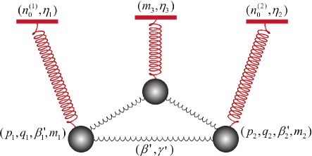
Figure 1: (Color online). Schematic illustration of the three coupled nonlinear pendulums.

We now adopt the mean-field approximation and define for each condensate species a mode function $\psi(\vec{r})$/$\phi(\vec{r})$, justified by the fact the spin independent density interaction terms are usually much stronger than spin dependent interactions. We therefore take $\Psi_{i}(\vec{r})\equiv\langle\hat{\Psi}_{i}(\vec{r})\rangle=\sqrt{n^{(1)}_{j}}\,e^{i\theta_{j}}\psi(\vec{r})$ and $\Phi_{i}(\vec{r})\equiv\langle\hat{\Phi}_{i}(\vec{r})\rangle=\sqrt{n^{(2)}_{j}}\,e^{i\varphi_{j}}\phi(\vec{r})$. The spin dynamics are then governed by the spin-dependent energy functional

$$\mathcal{E} = \sum_{j=1,2}\mathcal{E}_{j}+\mathcal{E}_{12},$$

$$\mathcal{E}_{j} = -p_{j}m_{j}+q_{j}(n_{j}-n_{0}^{(j)})+\frac{1}{2}\beta^{\prime}_{j}m_{j}^{2}$$

$$+\beta^{\prime}_{j}n_{0}^{(j)}\Big{[}(n_{j}-n_{0}^{(j)})+\sqrt{(n_{j}-n_{0}^{(j)})^{2}-m_{j}^{2}}\cos\eta_{j}\Big{]},$$

$$\mathcal{E}_{12} = \frac{1}{2}\beta^{\prime}m_{1}m_{2}+\frac{1}{6}\gamma^{\prime}(n_{1}^{(1)}n_{-1}^{(2)}+n_{0}^{(1)}n_{0}^{(2)}+n_{-1}^{(1)}n_{1}^{(2)})$$ (2)

$$+\frac{1}{3}\gamma^{\prime}\sqrt{n_{1}^{(1)}n_{-1}^{(1)}n_{1}^{(2)}n_{-1}^{(2)}}\cos\eta_{3},$$

$$+(\beta^{\prime}-\frac{1}{3}\gamma^{\prime})\sqrt{n_{0}^{(1)}n_{-1}^{(1)}n_{1}^{(2)}n_{0}^{(2)}}\cos(\frac{\eta_{1}+\eta_{2}+\eta_{3}}{2})$$

$$+(\beta^{\prime}-\frac{1}{3}\gamma^{\prime})\sqrt{n_{1}^{(1)}n_{0}^{(1)}n_{0}^{(2)}n_{-1}^{(2)}}\cos(\frac{\eta_{1}+\eta_{2}-\eta_{3}}{2})$$

$$+\beta^{\prime}\sqrt{n_{0}^{(1)}n_{-1}^{(1)}n_{0}^{(2)}n_{-1}^{(2)}}\cos(\frac{\eta_{1}-\eta_{2}+\eta_{3}}{2})$$

$$+\beta^{\prime}\sqrt{n_{1}^{(1)}n_{0}^{(1)}n_{1}^{(2)}n_{0}^{(2)}}\cos(\frac{\eta_{1}-\eta_{2}-\eta_{3}}{2}),$$

where $n_{1,2}=\sum_{j}n^{(1,2)}_{j}$, $m_{1,2}=n_{1}^{(1,2)}-n_{-1}^{(1,2)}$, $\eta_{1}=\theta_{1}+\theta_{-1}-2\theta_{0}$, $\eta_{2}=\varphi_{1}+\varphi_{-1}-2\varphi_{0}$, and $\eta_{3}=\theta_{-1}-\theta_{1}+\varphi_{1}-\varphi_{-1}$. The interaction parameters are now redefined to absorb the relevant multipliers: $\beta^{\prime}_{1}=\beta_{1}\int|\psi(\vec{r})|^{4}d\vec{r}$, $\beta^{\prime}_{2}=\beta_{2}\int|\phi(\vec{r})|^{4}d\vec{r}$, and $(\beta^{\prime},\gamma^{\prime})=(\beta,\gamma)\int|\psi(\vec{r})|^{2}|\phi(\vec{r})|^{2}d\vec{r}$. We note that $\int|\psi(\vec{r})|^{2}d\vec{r}=\int|\phi(\vec{r})|^{2}d\vec{r}=1$. When the two species are immersible, the overlaps between $\psi(\vec{r})$ and $\phi(\vec{r})$ is significantly reduced, leading to diminished $\beta^{\prime}$ and $\gamma^{\prime}$, essentially reducing the system to two stand-alone spin-1 condensates.

Although complicated in forms, the above Hamiltonian gives rise to dynamics that can be interpreted simply in terms of three coupled nonlinear pendulums, with three pairs of canonical variables: $(n_{0}^{(j)},\eta_{j})$ and $(m_{3}=m_{1}-m_{2},\eta_{3})$. Their corresponding equations of motion are given by

$$\dot{n}_{0}^{(j)}=-\frac{2}{\hbar}\frac{\partial\mathcal{E}}{\partial\eta_{j}}, \dot{\eta}_{j}=\frac{2}{\hbar}\frac{\partial\mathcal{E}}{\partial n_{0}^{(j)}},$$

$$\dot{m}_{3}=-\frac{4}{\hbar}\frac{\partial\mathcal{E}}{\partial\eta_{3}}, \dot{\eta}_{3}=\frac{4}{\hbar}\frac{\partial\mathcal{E}}{\partial m_{3}},$$ (3)

as illustrated schematically in Fig. 1.

III Determining the interspecies spin singlet-pairing interaction

When discussing spin mixing in a spin-2 condensate, Saito et al. saito2005 proposed to determine the value of intra-species spin singlet-pairing interaction by choosing an elementary process $0+0\leftrightarrow 2+(-2)$ which occurs only when the spin singlet-pairing interaction is non-vanishing. With a suitable initial state of zero magnetization, the mixing dynamics is governed by coupled first-order ordinary differential equations, which contain unknown parameters like singlet-pairing interactions and quadratic Zeeman shifts. The analytic solutions can be compared with the experimental measured dynamics to decide the unknowns.

Analogous approach can be taken to determine the value of interspecies spin singlet-pairing interaction for a binary mixture of spin-1 ⁸⁷Rb and ²³Na atom condensates, making use of a different elementary collision process $\Psi_{1}+\Phi_{-1}\leftrightarrow\Psi_{-1}+\Phi_{1}$ which appears only in the presence of the $\gamma^{\prime}$ term. With an initial state

$$\Psi/\psi=\left(\begin{array}[]{c}\sqrt{n_{1}^{(1)}}e^{i\theta_{1}}\\ 0\\ \sqrt{n_{-1}^{(1)}}e^{i\theta_{-1}}\end{array}\right),\quad\Phi_{j}/\phi=\left(\begin{array}[]{c}\sqrt{n_{1}^{(2)}}e^{i\varphi_{1}}\\ 0\\ \sqrt{n_{-1}^{(2)}}e^{i\varphi_{-1}}\end{array}\right),$$ (10)

$\psi_{0}$ and $\phi_{0}$ re found to remain exactly zero within the mean-field approximation, unless dynamical instabilities exist. If instabilities do occur, they can be suppressed by tuning the quadratic Zeeman shifts $q_{j}$ to a large negative value, for instance with off-resonant microwave field gerbier2006 ; leslie2009 , or to a large positive value with increased uniform B-field. The processes $\Psi_{1}+\Psi_{-1}\leftrightarrow\Psi_{0}+\Psi_{0}$ and $\Phi_{1}+\Phi_{-1}\leftrightarrow\Phi_{0}+\Phi_{0}$ will then be suppressed, the populations of the $M_{F}=0$ states remain at zero. In this case, the spin mixing dynamics of Eq. (3) reduce to that of a single pair, which takes the form,

$$\dot{m}_{3} = \frac{\gamma^{\prime}}{12\hbar}\sqrt{[4n_{1}^{2}-(m+m_{3})^{2}][4n_{2}^{2}-(m-m_{3})^{2}]}$$

$$\times\sin\eta_{3},$$

$$\dot{\eta}_{3} = \frac{\beta^{\prime}_{1}-\beta^{\prime}_{2}}{\hbar}m+\frac{\beta^{\prime}_{1}+\beta^{\prime}_{2}-\beta^{\prime}+\gamma^{\prime}/6}{\hbar}m_{3}$$ (11)

$$- \frac{\gamma^{\prime}}{6\hbar}\frac{2(n_{1}^{2}+n_{2}^{2})m_{3}-2(n_{1}^{2}-n_{2}^{2})m+m^{2}m_{3}-m_{3}^{3}}{\sqrt{[4n_{1}^{2}-(m+m_{3})^{2}][4n_{2}^{2}-(m-m_{3})^{2}]}}$$

$$\times\cos\eta_{3},$$

and is described by a simpler energy functional

$$\mathcal{E} = \frac{\beta^{\prime}_{1}+\beta^{\prime}_{2}-\beta^{\prime}+\gamma^{\prime}/6}{8}m_{3}^{2}+\frac{\beta^{\prime}_{1}-\beta^{\prime}_{2}}{4}mm_{3}$$ (12)

$$+ \frac{\gamma^{\prime}}{48}\sqrt{[4n_{1}^{2}-(m+m_{3})^{2}][4n_{2}^{2}-(m-m_{3})^{2}]}\cos\eta_{3},\hskip 12.0pt\quad$$

after neglecting a constant term $-pm+(\beta^{\prime}_{1}+\beta^{\prime}_{2}+\beta^{\prime}-\gamma^{\prime}/6)m^{2}/8+\gamma^{\prime}n_{1}n_{2}/12+q_{1}n_{1}+q_{2}n_{2}$. Substituting Eq. (12) into Eq. (11), we find

$$(\dot{m}_{3})^{2}=\left(\frac{\gamma^{\prime}}{12\hbar}\right)^{2}[4n_{1}^{2}-(m+m_{3})^{2}][4n_{2}^{2}-(m-m_{3})^{2}]$$

$$-\frac{16}{\hbar^{2}}\Big{[}\mathcal{E}-\frac{\beta^{\prime}_{1}+\beta^{\prime}_{2}-\beta^{\prime}+\gamma^{\prime}/6}{8}m_{3}^{2}-\frac{\beta^{\prime}_{1}-\beta^{\prime}_{2}}{4}mm_{3}\Big{]}^{2},$$ (13)

which can be integrated following the procedure of Ref. zhang2005a by solving for the equation $\dot{m}_{3}=0$, keeping the interspecies spin-dependent interaction parameters $\beta^{\prime}$ and $\gamma^{\prime}$ as unknown.

From the Eq. (11) and assuming an initial state with $\sin\eta_{3}>0$, we infer $\gamma^{\prime}>0$ if $m_{3}$ increases during the initial short time period of the spin mixing dynamics, and $\gamma^{\prime}<0$ if it decreases. To determine $\gamma^{\prime}$, we prepare an initial state with $\eta_{3}=\pi/2$ and $m_{1}=m_{2}=0$, which leads to $\mathcal{E}=0$ in the Eq. (12), and

$$(\dot{m}_{3})^{2}=\frac{\gamma^{\prime 2}}{144\hbar^{2}}\Big{[}(m_{3}^{2}-4n_{1}^{2})(m_{3}^{2}-4n_{2}^{2})-\mathcal{C}^{2}m_{3}^{4}\Big{]},$$ (14)

with $\mathcal{C}=|6(\beta^{\prime}_{1}+\beta^{\prime}_{2}-\beta^{\prime})/\gamma^{\prime}+1|$. If $\mathcal{C}<1$, $\dot{m}_{3}=0$ gives four roots $-x_{2}$, $-x_{1}$, $x_{1}$, and $x_{2}$, where $x_{1/2}=\sqrt{2\big{(}n_{1}^{2}+n_{2}^{2}\mp\sqrt{(n_{1}^{2}-n_{2}^{2})^{2}+4\mathcal{C}^{2}n_{1}^{2}n_{2}^{2}}\big{)}/(1-\mathcal{C}^{2})}$. For $\mathcal{C}\geq 1$, however, only two solutions $-x_{1}$ and $x_{1}$ exist. The solution for the mixing dynamics is expressed in terms of the Jacobian elliptic functions sn(.) and cn(.) as

$$m_{3}(t) = x_{1}\ {\rm sn}\left(\frac{x_{2}\gamma^{\prime}t\sqrt{1-\mathcal{C}^{2}}}{12\hbar},\frac{x_{1}}{x_{2}}\right),\text{for $\mathcal{C}\leq 1$},$$

$$m_{3}(t) = x_{1}\ {\rm cn}\left(K\Big{(}\frac{x_{1}}{\sqrt{x_{1}^{2}+x_{3}^{2}}}\Big{)}-\frac{\gamma^{\prime}t\sqrt{(x_{1}^{2}+x_{3}^{2})(\mathcal{C}^{2}-1})}{12\hbar},\right.$$ (15)

$$\qquad\left.\frac{x_{1}}{\sqrt{x_{1}^{2}+x_{3}^{2}}}\right),\text{for $\mathcal{C}\geq 1$},$$

where $K(.)$ is the complete elliptic integral of the first kind, and $x_{3}=\sqrt{2\big{(}n_{1}^{2}+n_{2}^{2}+\sqrt{(n_{1}^{2}-n_{2}^{2})^{2}+4\mathcal{C}^{2}n_{1}^{2}n_{2}^{2}}\big{)}/(\mathcal{C}^{2}-1)}$.

The stability of the above dynamics are confirmed with numerical solutions, taking the initial state as $\Psi_{j}/\psi=\sqrt{n_{1}}(1,0,1)^{T}/\sqrt{2}$, $\Phi_{j}/\phi=\sqrt{n_{2}}(1,0,-i)^{T}/\sqrt{2}$, assuming $n_{1}=n_{2}=n$ and $n=2\times 10^{4}$. We further choose $\beta^{\prime}_{1}/\hbar=-22.4893\times 10^{-4}\,\rm Hz$ and $\beta^{\prime}_{2}/\hbar=303.816\times 10^{-4}\,\rm Hz$. A noise level at $10^{-5}$ in the population of $M_{F}=0$ spin states of both species is also included. The B-field is set as large enough to suppress the intraspecies spin-exchange process with the quadratic Zeeman shifts satisfying $q_{1}=40|\beta^{\prime}_{1}|n$ and $q_{2}=q_{1}\Delta E_{1}/\Delta E_{2}$, where $\Delta E_{1}$ and $\Delta E_{2}$ are the hyperfine splittings of ⁸⁷Rb and ²³Na atoms respectively. Figure 2 illustrates our numerical results. In Fig. 2(a-c), $\beta^{\prime}=5|\beta^{\prime}_{1}|$ and $\gamma^{\prime}=2|\beta^{\prime}_{1}|$ are used, while $\beta^{\prime}=5|\beta^{\prime}_{1}|$ and $\gamma^{\prime}=-2|\beta^{\prime}_{1}|$ are used instead for Fig. 2 (d-f). The time evolution for each condensate species are shown in Fig. 2(a,d) and (b,e) respectively for ⁸⁷Rb and ²³Na atoms. The evolutions for $m_{3}$ are shown in Fig. 2(c) and (f), indeed they confirm our predictions based on the insights gained from analytical solutions that $m_{3}$ increases/decreases at the beginning when $\gamma^{\prime}>0$/$\gamma^{\prime}<0$. The numerical simulations denoted by solid blue lines agree well with analytical solutions of Eq. (15) denoted by red square symbols. We further note that $\dot{n}^{(1)}_{1}=-\dot{n}^{(1)}_{-1}=-\dot{n}^{(2)}_{1}=\dot{n}^{(1)}_{2}=\dot{m}_{3}/4$ with the initial state used in this case. As a result, we can determine the sign of $\gamma^{\prime}$ from the populations of arbitrary spin components and species.

Using Eq. (15), we can then proceed to determine the value of $\gamma^{\prime}$ if $\mathcal{C}^{2}=x_{1}^{2}-4n_{1}^{2}-4n_{2}^{2}+16n_{1}^{2}n_{2}^{2}/x_{1}^{2}$ is first determined from the oscillation amplitude of $m_{3}$. Afterwards, $\beta^{\prime}$ becomes partially determine to within the following two choices

$$\beta^{\prime}_{\mp} = \beta^{\prime}_{1}+\beta^{\prime}_{2}\mp(\mathcal{C}\mp 1)\gamma^{\prime}/6.$$ (16)

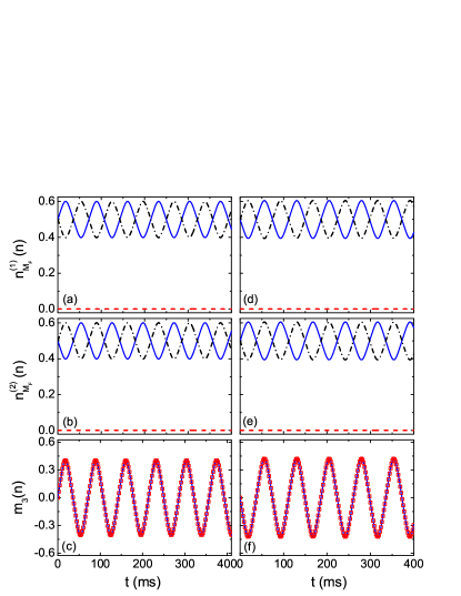
Figure 2: (Color online). Time dependent populations of each spin components. In the left panels of (a)-(c), the interspecies interaction parameters used are $\beta^{\prime}=5|\beta^{\prime}_{1}|$ and $\gamma^{\prime}=2|\beta^{\prime}_{1}|$. For the panels of (d)-(f), $\beta^{\prime}=5|\beta^{\prime}_{1}|$ and $\gamma^{\prime}=-2|\beta^{\prime}_{1}|$ are used. (a) For the ⁸⁷Rb condensate, where the solid blue line, dashed red line, and dotted-dash black line represent the $M_{F}=1,0,-1$ components, respectively. (b) As in (a), but for the ²³Na condensate. (c) Time dependent $m_{3}$ with solid blue line and red square symbols denote numerical and analytical solutions respectively. (d) As (a), but with $\gamma^{\prime}=-2|\beta^{\prime}_{1}|$. (e) As in (b), but with $\gamma^{\prime}=-2|\beta^{\prime}_{1}|$. (f) As in (c), but with $\gamma^{\prime}=-2|\beta^{\prime}_{1}|$.

IV Determining the interspecies spin-exchange interaction

In the previous section, a scheme is proposed capable of determining the interspecies singlet-pairing interaction parameter $\gamma^{\prime}$ following spin mixing dynamics from a suitably chosen initial state. The interspecies spin-exchange interaction parameter $\beta^{\prime}$, which is partially determined at the same time, will become fully determined with the dynamics discussed in this section.

Equation (2) gives four relevant elementary spin-exchange processes: $\Psi_{0}+\Phi_{0}\leftrightarrow\Psi_{-1}+\Phi_{1}$, $\Psi_{0}+\Phi_{0}\leftrightarrow\Psi_{1}+\Phi_{-1}$, $\Psi_{-1}+\Phi_{0}\leftrightarrow\Psi_{0}+\Phi_{-1}$, and $\Psi_{1}+\Phi_{0}\leftrightarrow\Psi_{0}+\Phi_{1}$, which can be used to determine the interspecies spin-exchange interaction. The first two processes involve both $\beta^{\prime}$ and $\gamma^{\prime}$ terms of the Hamiltonian in Eq. (1), while the last two processes are solely induced by spin-exchange interactions.

The above four individual processes become independent if all other possible collision channels are suppressed. For example, to observe the mixing due to $\Psi_{0}+\Phi_{0}\leftrightarrow\Psi_{-1}+\Phi_{1}$, $\Psi_{1}=\Phi_{-1}=0$ needs to be ensured at all times. A plausible scenario can again employ increased quadratic Zeeman shifts $q_{1}$ and $q_{2}$. As long as the energy difference between the final state and the initial state increases, the intraspecies spin-exchange process $\Psi_{1}+\Psi_{-1}\leftrightarrow\Psi_{0}+\Psi_{0}$ and $\Phi_{1}+\Phi_{-1}\leftrightarrow\Phi_{0}+\Phi_{0}$ are suppressed. They help to maintain close to zero populations during time evolution in the corresponding spin state, if an initial state with $\Psi_{1}=\Phi_{-1}=0$ is used.

In the following we will describe the isolation of the process $\Psi_{1}+\Phi_{0}\leftrightarrow\Psi_{0}+\Phi_{1}$ as an example to determine the interspecies spin-exchange interaction. An initial state

$$\Psi/\psi=\left(\begin{array}[]{c}\sqrt{n_{1}^{(1)}}e^{i\theta_{1}}\\ \sqrt{n_{0}^{(1)}}e^{i\theta_{0}}\\ 0\end{array}\right),\quad\Phi/\phi=\left(\begin{array}[]{c}\sqrt{n_{1}^{(2)}}e^{i\varphi_{1}}\\ \sqrt{n_{0}^{(2)}}e^{i\varphi_{0}}\\ 0\end{array}\right),$$ (23)

is assumed, together with a sufficiently strong uniform external magnetic field to guarantee $\Psi_{-1}=\Phi_{-1}=0$. Since interspecies spin mixing is only induced by the same $\beta^{\prime}$ term, and energy conservation, the spin mixing dynamics is then governed by the evolution of $m_{3}$

$$\dot{m}_{3} = -\frac{\beta^{\prime}}{2\hbar}\sqrt{(m^{2}-m_{3}^{2})(2n_{1}-m-m_{3})(2n_{2}-m+m_{3})}$$ (24)

$$\times\sin\frac{\eta_{1}-\eta_{2}-\eta_{3}}{2},$$

which can be derived from the Eq. (3), and the associated energy functional

$$\mathcal{E} = -\frac{\beta^{\prime}_{1}+\beta^{\prime}_{2}+\beta^{\prime}}{8}m_{3}^{2}-\frac{\beta^{\prime}_{1}-\beta^{\prime}_{2}}{4}mm_{3}+\frac{\beta^{\prime}_{1}n_{1}+q_{1}}{2}m_{3}$$ (25)

$$- \frac{\beta^{\prime}_{2}n_{2}+q_{2}}{2}m_{3}+\frac{\gamma^{\prime}}{24}(2n_{1}-m-m_{3})(2n_{2}-m+m_{3})$$

$$+ \frac{\beta^{\prime}}{4}\sqrt{(m^{2}-m_{3}^{2})(2n_{1}-m-m_{3})(2n_{2}-m+m_{3})}$$

$$\times\cos\frac{\eta_{1}-\eta_{2}-\eta_{3}}{2},$$

after neglecting a constant term $-pm-(\beta^{\prime}_{1}+\beta^{\prime}_{2}-\beta^{\prime})m^{2}/8+(\beta^{\prime}_{1}n_{1}+\beta^{\prime}_{2}n_{2}+q_{1}+q_{2})m/2$. Furthermore we can rewrite Eq. (24) as

$$(\dot{m}_{3})^{2} = \frac{\beta^{\prime 2}}{4\hbar^{2}}(m^{2}-m_{3}^{2})(2n_{1}-m-m_{3})(2n_{2}-m+m_{3})$$ (26)

$$- \frac{4}{\hbar^{2}}\Big{[}\mathcal{E}+\frac{\beta^{\prime}_{1}+\beta^{\prime}_{2}+\beta^{\prime}}{8}m_{3}^{2}+\frac{\beta^{\prime}_{1}-\beta^{\prime}_{2}}{4}mm_{3}$$

$$\quad\quad-\frac{\gamma^{\prime}}{24}(2n_{1}-m-m_{3})(2n_{2}-m+m_{3})$$

$$\quad\quad-\frac{\beta^{\prime}_{1}n_{1}+q_{1}}{2}m_{3}+\frac{\beta^{\prime}_{2}n_{2}+q_{2}}{2}m_{3}\Big{]}^{2}.$$

The procedure to fully determine $\beta^{\prime}$ goes as follows. First we infer the sign of $\beta^{\prime}$ from the initial stage of the time evolution for $m_{3}$, as in the earlier section on determining the sign of $\gamma^{\prime}$. For an initial state with $\Psi/\psi=\sqrt{n_{1}}(1,1,0)^{T}/\sqrt{2}$ and $\Phi/\phi=\sqrt{n_{2}}(1,-i,0)^{T}/\sqrt{2}$, where $(\eta_{1}-\eta_{2}-\eta_{3})/2=\theta_{1}-\theta_{0}-\varphi_{1}+\varphi_{0}=-\pi/2$, we confirm $\beta^{\prime}>0$ ($\beta^{\prime}<0$) if $m_{3}$ initially increases (decreases). The actual value of $\beta^{\prime}$ is determined by comparing the analytic or numerical solutions using the two choices of $\beta^{\prime}$ from the Eq. (16) to experimental measurements. Again we assume $n_{1}=n_{2}=n=2\times 10^{4}$, $\beta^{\prime}_{1}/\hbar=-22.4893\times 10^{-4}\,\rm Hz$, $\beta^{\prime}_{2}/\hbar=303.816\times 10^{-4}\,\rm Hz$, $\beta^{\prime}=5|\beta^{\prime}_{1}|$, $\gamma^{\prime}=2|\beta^{\prime}_{1}|$, $q_{1}=30|\beta^{\prime}_{1}|n$, and $q_{2}=q_{1}\Delta E_{2}/\Delta E_{1}$, with the analytic solution for $m_{3}$

$$m_{3}(t) = \frac{x_{1}(x_{2}-x_{4})+(x_{1}-x_{2})x_{4}x^{2}}{(x_{2}-x_{4})+(x_{1}-x_{2})x^{2}},$$

$$x = {\rm sn}\left(d_{4}-t\sqrt{d_{3}}/d_{2},d_{1})\right),$$ (27)

where $x_{j=1,2,3,4}$ are the four roots of $\dot{m}_{3}=0$, arranged in descending order $x_{1}>0>x_{2}>x_{3}>x_{4}$, and $d_{1}=\sqrt{(x_{1}-x_{2})(x_{3}-x_{4})/(x_{1}-x_{3})/(x_{2}-x_{4})}$, $d_{2}=2/\sqrt{(x_{1}-x_{3})(x_{2}-x_{4})}$, $d_{3}=[4\beta^{\prime 2}-(\beta^{\prime}_{1}+\beta^{\prime}_{2}+\beta^{\prime}+\gamma^{\prime}/3)^{2}]/16\hbar^{2}$, and $d_{4}={\rm F}(\arcsin\sqrt{-(x_{2}-x_{4})x_{1}/(x_{1}-x_{2})/x_{4}},d_{1})$, with F(.) the elliptic integral of the first kind.

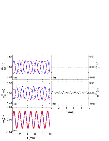
Figure 3: (Color online). Population dynamics for all spin components, with the interspecies interaction parameters $\beta^{\prime}=5|\beta^{\prime}_{1}|$ and $\gamma^{\prime}=2|\beta^{\prime}_{1}|$, and the quadratic Zeeman shifts $q_{1}=30|\beta^{\prime}_{1}|n$ and $q_{2}=q_{1}\Delta E_{2}/\Delta E_{1}$. (a) For the ⁸⁷Rb condensate, where the solid blue line and dashed red line represent the $M_{F}=1,0$ components, respectively. (b) As in (a), but for the $M_{F}=-1$ component in dotted-dash black line. (c)/(d) corresponds to that in (a)/(b) respectively, but for the ²³Na condensate. (e) Time evolution of $m_{3}$, where solid blue line and red square symbols denote numerical and analytical solutions respectively.

Figure 3 show population evolutions for all spin components. Due to the large but unequal quadratic Zeeman shifts $q_{1}$ and $q_{2}$, the suppression of intraspecies spin mixing dynamics leads to a suppressed amplitude for interspecies spin-exchange dynamics. As a result, the quadratic Zeeman shifts cannot be tuned too large, otherwise they cause nonzero populations in the $M_{F}=-1$ spin component especially for the ²³Na atoms as illustrated in Fig. 3(d).

The other three elementary channels can also be employed to determine the interspecies spin-exchange interaction. Among them, two are capable of determining the combined parameter $\beta^{\prime}-\gamma^{\prime}/3$, which can be further aided by a determination of the sign of $\beta^{\prime}-\gamma^{\prime}/3$.

Before conclusion, we hope to stress that the special mixture illustrated in this study involves a spin-1 condensate with ferromagnetic interaction (⁸⁷Rb) and a polar spin-1 condensate (²³Na) with antiferromagnetic interaction. More generally the procedures we suggest for determine the interspecies interaction parameters remain applicable for mixtures with two spin-1 ferromagnetic condensates or two antiferromagnetic condensates.

V Conclusion

We discuss coherent spin mixing dynamics for a binary mixture of spin-1 condensates. Under the mean field approximation, the dynamics reduce to three coupled nonlinear pendulums, one for each spin-1 condensate as understood previously for stand-alone spin-1 condensate zhang2005a , and a third one for the difference in magnetization between the two species. By tuning quadratic Zeeman shifts to large enough values, they can suppress intraspecies spin mixing dynamics, which results in a pure interspecies spin mixing dynamics. Using suitably prepared initial states with zero populations in the $M_{F}=0$ states for both species, we can determine the value of the interspecies singlet-pairing interaction by comparing the analytic formula to experimental measurements, and at the same time we can partially determine the value of the interspecies spin-exchange interaction parameter $\beta^{\prime}$. Next, using an alternative initial state with zero populations in the $M_{F}=-1$ states of both species, and using the two possible values for $\beta^{\prime}$ partially determined above, we can numerically or analytically solve the dynamics and compare them with experimental results to determine the correct value of $\beta^{\prime}$.

VI Acknowledgements

This work is supported by NSF of China under Grant No. 11004116, No. 91121005, NKBRSF of China, and the research program 2010THZO of Tsinghua University. D. W. is supported by Hong Kong RGC CUHK 403111.

References

• (1) I. Žutić, J. Fabian, S. Das Sarma, Rev. Mod. Phys. 76, 323 (2004).
• (2) M. Ueda and Y. Kawaguchi, e-print arXiv: 1001.2072.
• (3) Tin-Lun Ho, Phys. Rev. Lett. 81, 742 (1998).
• (4) T. Ohmi and K. Machida, J. Phys. Soc. Jpn. 67, 1822 (1998).
• (5) C. K. Law, H. Pu, and N. P. Bigelow, Phys. Rev. Lett. 81, 5257 (1998).
• (6) Masato Koashi and Masahito Ueda, Phys. Rev. Lett. 84, 1066 (2000).
• (7) C. V. Ciobanu, S.-K.Yip, and Tin-Lun Ho, Phys. Rev. A 61, 033607 (2000).
• (8) M. Ueda and M. Koashi, Phys. Rev. A 65, 063602 (2002).
• (9) A. M. Rey, V. Gritsev, I. Bloch, E. Demler, and M. D. Lukin, Phys. Rev. Lett. 99, 140601 (2007).
• (10) Wenxian Zhang, D. L. Zhou, M.-S. Chang, M. S. Chapman, and L. You, Phys. Rev. Lett. 95, 180403 (2005).
• (11) L. E. Sadler, J. M. Higbie, S. R. Leslie, M. Vengalattore, and D. M. Stamper-Kurn, Nature 443, 312 (2006).
• (12) C. Gross, T. Zibold, E. Nicklas, J. Estève, and M. K. Oberthaler, Nature 464, 1165 (2010).
• (13) M. F. Riedel, P. Böhi, Y. Li, T. W. Hänsch, A. Sinatra, and P. Treutlein, Nature 464, 1170 (2010).
• (14) M. D. Barrett, J. A. Sauer, and M. S. Chapman, Phys. Rev. Lett. 87, 010404 (2001).
• (15) M.-S. Chang, C. D. Hamley, M. D. Barrett, J. A. Sauer, K. M. Fortier, W. Zhang, L. You, and M. S. Chapman, Phys. Rev. Lett. 92, 140403 (2004).
• (16) M.-S. Chang, Q. Qin, W. Zhang, L. You, M. S. Chapman, Nature Physics 1, 111 (2005).
• (17) J. Kronjäger, C. Becker, M. Brinkmann, R. Walser, P. Navez, K. Bongs, and K. Sengstock, Phys. Rev. A 72, 063619 (2005).
• (18) Y. Liu, S. Jung, S. E. Maxwell, L. D. Turner, E. Tiesinga, and P. D. Lett, Phys. Rev. Lett. 102, 125301 (2009).
• (19) A. Widera, F. Gerbier, S. Fölling, T. Gericke, O. Mandel and I. Bloch, New J. Phys. 8, 152 (2006).
• (20) H. Schmaljohann, M. Erhard, J. Kronjäger, M. Kottke, S. van Staa, L. Cacciapuoti, J. J. Arlt, K. Bongs, and K. Sengstock, Phys. Rev. Let. 92, 040402 (2004).
• (21) T. Kuwamoto, K. Araki, T. Eno, and T. Hirano, Phys. Rev. A 69, 063604 (2004).
• (22) J. Kronjäger, C. Becker, P. Navez, K. Bongs, and K. Sengstock, Phys. Rev. Lett. 97, 110404 (2006).
• (23) S. Yi, Ö. E. Müstecaplıoğlu, C. P. Sun, and L. You, Phys. Rev. A 66, 011601(R) (2002).
• (24) D. R. Romano and E. J. V. de Passos, Phys. Rev. A 70, 043614 (2004).
• (25) W. Zhang, D. L. Zhou, M.-S. Chang, M. S. Chapman, and L. You, Phys. Rev. A 72, 013602 (2005).
• (26) H. Saito and M. Ueda, Phys. Rev. A 72, 053628 (2005).
• (27) M. Luo, Z. Li, and C. Bao, Phys. Rev. A 75, 043609 (2007).
• (28) Z. F. Xu, Yunbo Zhang, and L. You, Phys. Rev. A 79, 023613 (2009).
• (29) Z. F. Xu, Jie Zhang, Yunbo Zhang, and L. You, Phys. Rev. A 81, 033603 (2010).
• (30) Jie Zhang, Z. F. Xu, L. You, and Yunbo Zhang, Phys. Rev. A 82, 013625 (2010).
• (31) Z. F. Xu, J. W. Mei, R. Lü, and L. You, Phys. Rev. A 82, 053626 (2010).
• (32) Yu Shi, Phys. Rev. A 82, 023603 (2010).
• (33) Z. F. Xu, R. Lü, and L. You, Phys. Rev. A 84, 063634 (2011).
• (34) H. T. C. Stoof, J. M. V. A. Koelman, and B. J. Verhaar, Phys. Rev. B 38, 4688 (1988).
• (35) S. B. Weiss, M. Bhattacharya, and N. P. Bigelow, Phys. Rev. A 68, 042708 (2003).
• (36) A. Pashov, O. Docenko, M. Tamanis, R. Ferber, H. Knöckel, and E. Tiemann, Phys. Rev. A 72, 062505 (2005).
• (37) For 87Rb atoms $a_{0}100.4(a_{B})$, $a_{2}=101.8(a_{B})$, as taken from E. G. M. van Kempen, S. J. J. M. F. Kokkelmans, D. J. Heinzen and B. J. Verhaar, Phys. Rev. Lett. 88, 093201 (2002).
• (38) For 23Na atoms $a_{0}=50.0(a_{B})$, $a_{2}=55.0(a_{B})$, as taken from A. Crubellier, O. Dulieu, F. Masnou-Seeuws, M. Elbs, H. Knockel and E. Tiemann, Eur. Phys. J. D 6, 211 (1999).
• (39) F. Gerbier, A. Widera, S. Fölling, O. Mandel, and I. Bloch, Phys. Rev. A 73, 041602(R) (2006).
• (40) S. R. Leslie, J. Guzman, M. Vengalattore, J. D. Sau, M. L. Cohen, and D. M. Stamper-Kurn, Phys. Rev. A 79, 043631 (2009).