Element orbitals for Kohn-Sham density functional theory

Abstract

We present a method to discretize the Kohn-Sham Hamiltonian matrix in the pseudopotential framework by a small set of basis functions automatically contracted from a uniform basis set such as planewaves. Each basis function is localized around an element, which is a small part of the global domain containing multiple atoms. We demonstrate that the resulting basis set achieves meV accuracy for 3D densely packed systems with a small number of basis functions per atom. The procedure is applicable to insulating and metallic systems.

I Introduction

Kohn-Sham density functional theory (KSDFT) Kohn and Sham (1965) is the most widely used electronic structure theory for condensed matter systems. When solving the Kohn-Sham equations, the choice of basis functions usually poses a dilemma for practitioners. The accurate and systematically improvable basis functions that are uniform in space, such as plane waves or finite elements, typically result in a large number of degrees of freedom ($500\sim 10000$) per atom in the framework of norm conserving pseudopotential Troullier and Martins (1991) especially for transition metal elements. The number of basis functions per atom can be reduced to the order of hundreds using ultrasoft pseudopotential Vanderbilt (1990), or augmentation techniques in the core-region such as the linearized augmented plane-wave (LAPW) method Andersen (1975) and the projector augmented wave (PAW) method Blöchl (1994). The relatively large number of basis functions used leads to a large prefactor in front of the already expensive cubic scaling for solving KSDFT.

Contracted basis functions, such as Gaussian type orbitals, atomic orbitals or muffin-tin orbitals, can represent the Kohn-Sham orbitals with a small number of degrees of freedom per atom ($4\sim 100$). These contracted basis functions contain a number of parameters to be determined. The flexibility for choosing different forms of parameters has generated a vast amount of literature (see e.g. Refs. Ozaki, 2003; Blum et al., 2009; Junquera et al., 2001; Chen et al., 2010; Andersen and Saha-Dasgupta, 2000; Qian et al., 2008) in the past few decades, which has been reviewed recently in Ref. Bowler and Miyazaki, 2012. The parameters in the contracted basis functions are typically constructed by a fitting procedure for a range of reference systems. The necessary inclusion of polarization basis Frisch et al. (1984), diffuse basis  Clark et al. (1983), multiple radial functions for each angular momentum (multiple $\zeta$ basis Junquera et al. (2001)) are just a few examples when the choice of basis functions becomes difficult and system dependent especially for complex systems.

It is desirable to combine the advantage of uniform basis set in which the accuracy is controlled by no more than a handful of universal parameters for almost all materials, and the advantage of contracted basis functions with a very small number of basis functions per atom. In other words, we would like to generate a small number of contracted basis functions by a unified procedure with high accuracy comparable to that obtained from uniform basis functions. In a recent work Lin et al. (2012a), we have developed a unified method for constructing a set of contracted basis functions from a uniform basis set such as planewaves in the pseudopotential framework. The new basis set, called adaptive local basis (ALB) set, is constructed by solving the Kohn-Sham problem restricted to a small part of the domain called element. Each ALB is discontinuous from the perspective of the global domain, and the continuous Kohn-Sham orbitals are approximated by the discontinuous ALBs under a discontinuous Galerkin framework Arnold (1982). It was demonstrated that the ALBs are able to achieve high accuracy (in the order of $1$ meV) using disordered Na and Si as examples. However, the number of basis functions per atom increases with respect to dimensionality. For example, $40$ basis functions per atom is needed to reach the accuracy of $1$ meV/atom for 3D bulk Na system.

In this paper, we propose a new basis set that is constructed from linear combination of adaptive local basis functions. Each new basis function, dubbed element orbital (EO), has localized nature around its associated element of the domain. The number of EOs used is significantly reduced compared to the number of ALBs for 3D bulk systems. We demonstrate that $4$ EOs per atom are sufficient to achieve $1$ meV per atom accuracy for 3D bulk Na system with disorderedness. We also apply EOs to study Na, Si and graphene, with varying system sizes, lattice constants or types of defects. The new method consistently achieves meV accuracy for calculating the total energy when compared to standard electronic structure software such as ABINIT Gonze et al. (2009). Since the EOs are contracted from a uniform basis set such as planewave basis set, the shape of the EOs has more flexibility to reflect the environmental effect than contracted basis sets which are centered around atoms. Numerical result indicates that the shape of EOs can resemble both atomic orbitals of different angular momentum and chemical bonds centered in the interstitial region, depending on their chemical environment.

We remark that the construction of the EOs is closely related to several existing techniques for reducing the number of basis functions per atom, starting from a large primitive basis set consisting of Gaussian orbitals or atomic orbitals Ozaki (2003); Blum et al. (2009); Rayson and Briddon (2009); Rayson (2010). However, the EOs are contracted from a fine uniform basis set such as planewaves, and a number of difficulties arise which makes the previous techniques difficult to be directly applied. For instance, the filtration technique in Ref. Rayson and Briddon, 2009; Rayson, 2010 constructs a near-minimal basis set from a large number of Gaussian type orbitals by applying a filtration matrix to a set of trial orbitals, taken from one or a few Gaussian-type orbitals. When the Gaussian-type orbitals are replaced by a fine uniform basis set such as planewaves, finding a good set of trial orbitals itself becomes a difficult task, and the construction of trial orbitals can inevitably introduce a set of undetermined parameters, which is not desirable in the current framework.

This paper is organized as follows: Section II introduces the adaptive local absis functions in the discontinuous Galerkin framework for solving Kohn-Sham density functional theory in the pseudopotential framework. The construction of the element orbitals is introduced in Section III. Section IV discusses briefly the implementation procedure of element orbitals. The performance of element orbitals is reported in Section V, followed by the discussion and conclusion in Section VI.

II Adaptive local basis functions

Consider a quantum system with $N$ electrons under external potential by $V_{\mathrm{ext}}$ in a rectangular domain $\Omega$ with periodic boundary condition. To simplify the equations, we ignore the electron spin for now. In Kohn-Sham density functional theory at a finite $T=1/(k_{B}\beta)$ Kohn and Sham (1965); Mermin (1965), the Helmholtz free energy is given by

$$\mathcal{F}_{\mathrm{tot}}=\mathcal{F}_{\mathrm{tot}}(\{\psi_{i}\},\{f_{i}\})=\frac{1}{2}\sum_{i}f_{i}\int\lvert\nabla\psi_{i}(x)\rvert^{2}\,\mathrm{d}x\\ +\int V_{\mathrm{ext}}(x)\rho(x)\,\mathrm{d}x+\sum_{\ell}\gamma_{\ell}\sum_{i}f_{i}\lvert\int b_{\ell}^{\ast}(x)\psi_{i}(x)\,\mathrm{d}x\rvert^{2}\\ +\frac{1}{2}\iint\frac{\rho(x)\rho(y)}{\lvert x-y\rvert}\,\mathrm{d}x\,\mathrm{d}y+\int\epsilon_{\mathrm{xc}}[\rho(x)]\,\mathrm{d}x\\ +\beta^{-1}\sum_{i}\bigl{(}f_{i}\ln f_{i}+(1-f_{i})\ln(1-f_{i})\bigr{)},$$ (1)

Correspondingly $\{\psi_{i}(x)\}$ and $\{f_{i}\}$ are the solutions to the minimization problem

$$\begin{split}&\min_{\{\psi_{i}\},\{f_{i}\}}\mathcal{F}_{\mathrm{tot}}(\{\psi_{i}\},\{f_{i}\}),\\ &\text{s.t.}\quad\int\psi_{i}^{\ast}(x)\psi_{j}(x)\,\mathrm{d}x=\delta_{ij},\quad i,j=1,\cdots,\widetilde{N}.\end{split}$$ (2)

$\{f_{i}\}\in[0,1]$ are the occupation numbers which add up to the total number of electrons $N=\sum_{i=1}^{\widetilde{N}}f_{i}$. Here we use exchange-correlation functional under local density approximation (LDA) Ceperley and Alder (1980); Perdew and Zunger (1981) and adopt norm conserving pseudopotential Troullier and Martins (1991), with the projection vector of the nonlocal pseudopotential in the Kleinman-Bylander form Kleinman and Bylander (1982) denoted by $\{b_{\ell}(x)\}$, and $\gamma_{\ell}=\pm 1$ is a sign. The number of eigenstates $\widetilde{N}$ calculated in practice is chosen to be slightly larger than the number of electrons $N$ in order to compensate for the finite temperature effect, following the criterion that the occupation number $f_{\widetilde{N}}$ is sufficiently small (less than $10^{-8})$. The electron density is given by

$$\rho(x)=\sum_{i=1}^{\widetilde{N}}f_{i}\lvert\psi_{i}(x)\rvert^{2}.$$

The Kohn-Sham equation, or the Euler-Lagrange equation associated with (2) is Kohn and Sham (1965); Mermin (1965)

$$H[\rho]\psi_{i}=\Bigl{(}-\tfrac{1}{2}\Delta+V_{\mathrm{eff}}[\rho]+\sum_{\ell}\gamma_{\ell}\lvert b_{\ell}\rangle\langle b_{\ell}\rvert\Bigr{)}\psi_{i}=\lambda_{i}\psi_{i},$$ (3)

where the effective one-body potential $V_{\mathrm{eff}}[\rho]$ is

$$V_{\mathrm{eff}}[\rho](x)=V_{\mathrm{ext}}(x)+\int\frac{\rho(y)}{\lvert x-y\rvert}\,\mathrm{d}y+\epsilon_{\mathrm{xc}}^{\prime}[\rho(x)]$$

and the occupation numbers $\{f_{i}\}_{i\geq 1}$ follow the Fermi-Dirac distribution

$$f_{i}=\frac{1}{1+\exp(\beta(\lambda_{i}-\mu))}.$$

Here the chemical potential $\mu$ is chosen so that $\sum_{i=1}^{\widetilde{N}}f_{i}=N$. In each SCF iteration of (3), we freeze $\rho$ and solve for the $\tilde{N}$ lowest eigenfunctions $\{\psi_{i}(x)\}_{1\leq i\leq\tilde{N}}$. This linear eigenvalue problem is the focus of the following discussion.

The discontinuous Galerkin (DG) framework Arnold (1982) provides flexibility in choosing appropriate basis functions to discretize the Kohn-Sham Hamiltonian $H[\rho]$. In the DG framework, a smooth function delocalized across the global domain can be systematically approximated by a set of discontinuous functions that are localized in the real space. Let $\mathcal{T}=\{E_{1},E_{2},\cdots,E_{M}\}$ be a collection of elements, i.e. disjoint rectangular partitions of $\Omega$, and $\mathcal{S}$ be the collection of surfaces $\{\partial E_{k}\}$ that correspond to each element $E_{k}$ in $\mathcal{T}$. We associate with each $E_{k}$ a set of orthogonal basis functions $\{u_{k,j}(x)\}_{1\leq j\leq J_{k}}$ supported in $E_{k}$, with the total number of basis functions given by

$$N^{b}=\sum_{k=1}^{M}J_{k}.$$

Under such a basis set, the Hamiltonian is discretized into an $N^{b}\times N^{b}$ matrix with entries given by

$$\begin{split}&\mathsf{H}(k^{\prime},j^{\prime};k,j)\\ =&\frac{1}{2}\left\langle\nabla u_{k^{\prime},j^{\prime}},\nabla u_{k,j}\right\rangle_{\mathcal{T}}-\frac{1}{2}\left\langle[[u_{k^{\prime},j^{\prime}}]],\{\{\nabla u_{k,j}\}\}\right\rangle_{\mathcal{S}}\\ &-\frac{1}{2}\left\langle\{\{\nabla u_{k^{\prime},j^{\prime}}\}\},[[u_{k,j}]]\right\rangle_{\mathcal{S}}+\alpha\left\langle[[u_{k^{\prime},j^{\prime}}]],[[u_{k,j}]]\right\rangle_{\mathcal{S}}\\ &+\left\langle u_{k^{\prime},j^{\prime}},V_{\mathrm{eff}}u_{k,j}\right\rangle_{\mathcal{T}}+\sum_{\ell}\gamma_{\ell}\left\langle u_{k^{\prime},j^{\prime}},b_{\ell}\right\rangle_{\mathcal{T}}\left\langle b_{\ell},u_{k,j}\right\rangle_{\mathcal{T}},\end{split}$$ (4)

where $\left\langle\cdot,\cdot\right\rangle_{\mathcal{T}}$ and $\left\langle\cdot,\cdot\right\rangle_{\mathcal{S}}$ are inner products in the bulk and on the surface respectively, and $\alpha>0$ is a fixed parameter for penalizing cross-element discontinuity. The notations $\{\{\cdot\}\}$ and $[[\cdot]]$ stand for the average and jump operators across surfaces Arnold (1982). Comparing (3) and (4), the new terms involving the average and jump operators can be derived from integration by parts of the Laplacian operator, and provide consistency and stability of the DG method Arnold et al. (2002).

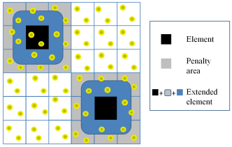
Figure 1: (color online) Sketch for the construction of adaptive local basis functions and element orbitals. Each adaptive local basis function is supported in an element. Each element orbital is supported in an extended element.

In the work of adaptive local basis set Lin et al. (2012a), the functions $\{u_{k,j}\}_{1\leq j\leq J_{k}}$ in each element $E_{k}$ are determined as follows. Let $d$ be the dimension of the system. For each $E_{k}$ (one black box in Fig. 1), we define an associated extended element $Q_{k}$, which includes both $E_{k}$ and its $3^{d}-1$ neighboring elements. Define $H_{Q_{k}}[\rho]$ to be the restriction of $H[\rho]$ to $Q_{k}$ with periodic boundary condition and with potential given by the restriction of $V_{\mathrm{eff}}[\rho]$ to $Q_{k}$. $H_{Q_{k}}[\rho]$ is then discretized and diagonalized with uniform basis functions such as planewaves. We denote the corresponding eigenvalues and eigenfunctions by $\{\lambda_{k,j}\}_{j\geq 1}$ and $\{\varphi_{k,j}(x)\}_{j\geq 1}$, respectively, starting from the lowest eigenvalue. One then restricts the first $J_{k}$ functions of $\{\varphi_{k,j}(x)\}_{j\geq 1}$ to $E_{k}$, where $J_{k}$ is set to be proportional to the number of electrons inside the extended element $Q_{k}$ (see the numerical examples for specific choice of $J_{k}$). In addition, we define for each $E_{k}$

$$\lambda_{k}^{c}=\lambda_{k,J_{k}},$$ (5)

i.e. the largest selected eigenvalue in $E_{k}$ which shall be used later. Applying the Gram-Schmidt procedure to $\{\varphi_{k,j}(x)\}_{1\leq j\leq J_{k}}$ then gives rise to a set of orthonormal functions

$$\{u_{k,j}(x)\}_{1\leq j\leq J_{k}}$$ (6)

for each $E_{k}$. The union of such functions over all elements $\{u_{k,j}(x)\}_{1\leq k\leq M,1\leq j\leq J_{k}}$ gives the set of adaptive local basis functions (ALBs).

For a given system, the partition of $E_{k}$ is kept to be the same even with changing atomic configurations as in the case of structure optimization and molecular dynamics. Dangling bonds may form when atoms are present on the surface of the extended elements, but we emphasize that these dangling bonds are not needed to be passivated by introducing auxiliary atoms near the surface of the extended elements Zhao et al. (2008). This is because the potential is not obtained self-consistently within $Q_{k}$, but instead from the restriction of the screened potential in the global domain $\Omega$ to $Q_{k}$ in each SCF iteration, which mutes the catastrophic damage of the dangling bonds. The oscillation in the basis functions caused by the discontinuity of the potential at the surface of the $Q_{k}$ (called Gibbs phenomenon) still exists, but it damps exponentially away from the surface of $Q_{k}$ and has controlled effect in $E_{k}$. Using disordered Na and Si as examples, we demonstrated that ALB can achieve meV accuracy per atom using $4\sim 40$ basis functions per atom Lin et al. (2012a).

III Element orbitals

The high accuracy of ALBs indicates that the span of $\{u_{k,j}\}_{1\leq k\leq M,1\leq j\leq J_{k}}$ approximately contains the span of the Kohn-Sham orbitals $\{\psi_{i}\}_{1\leq i\leq\tilde{N}}$. However, we found that the number of basis functions per atom may vary significantly with respect to the dimensionality $d$ of the system, which has not been seen reported in the literature using traditional contracted basis set to the extent of our knowledge.

The dimension dependence of ALBs can be intuitively understood as follows, motivated from the success of the contracted basis set such as atomic orbitals. Consider the case where an atom is positioned at the center of element $E_{k}$ and assume for simplicity that each of its atomic orbital overlaps only with the neighboring elements (i.e., those inside the extended element $Q_{k}$). In order to include one such atomic orbital denoted by $\eta(x)$ in the span of $\{u_{k,j}(x)\}_{1\leq k\leq M,1\leq j\leq J_{k}}$, each neighboring element $E_{k^{\prime}}$ in $Q_{k}$ should allocate one of its ALBs for representing the restriction of $\eta(x)$ in $E_{k^{\prime}}$. This implies that $N^{b}$, the total number of ALBs, should roughly be equal to $3^{d}\tilde{N}$, which becomes increasingly redundant with respect to the dimension $d$. In fact, this is close to what has been observed in the numerical experiments Lin et al. (2012a).

In order to avoid this redundancy and motivated by the construction of atomic orbitals, we propose to build a new basis set by piecing the ALBs in neighboring elements $\{E_{k^{\prime}}\}$ in $Q_{k}$ to construct functions that are qualitatively close to the atomic orbitals. To distinguish them from the pre-fitted atomic orbitals, we name these functions element orbitals (EOs). In order to achieve this, one is faced mainly with three issues. First, the ALBs are always discontinuous across the element boundaries, while qualitatively the EOs should be a continuous function since the atomic orbitals are continuous. Second, when one pieces back the ALBs to obtain the EOs, it is essential that the resulting functions have low-energy. Finally, one needs to make sure that the EOs of $E_{k}$ should be localized at $E_{k}$ in order to avoid degeneracy.

A two-step procedure is proposed to address these three issues. In the first step, we construct, for each element $E_{k}$, a set of candidate functions that take care of the first two issues. Then in the second step, we identify the element orbitals by localizing the candidate functions. More specifically, the method proceeds as follows.

Let us fix an element $E_{k}$. First, since each ALB is only supported in its associated element and equal to zero outside, we seek for a set of candidate functions for element $E_{k}$ that are linear combinations of the ALBs of both $E_{k}$ and its $3^{d}-1$ neighbors (Fig. 1). Denoting by $\mathcal{I}$ the index of all the ALBs, and by $\mathcal{I}_{k}\subset\mathcal{I}$ the index set of ALBs supported in $Q_{k}$, we define a local Hamiltonian

$$\mathsf{H}_{k}=\mathsf{H}(\mathcal{I}_{k},\mathcal{I}_{k}),$$

i.e., the restriction of $\mathsf{H}$ to the index set $\mathcal{I}_{k}$. Following the intuition that the atomic orbitals should only be affected by the local environment of $E_{k}$, it is reasonable to assume that the low eigenfunctions of $\mathsf{H}_{k}$ serve as good candidate functions. Computationally, we diagonalize $\mathsf{H}_{k}$ by

$$\mathsf{H}_{k}\mathsf{M}_{k}=\mathsf{M}_{k}\mathsf{\Delta}_{k},$$ (7)

where the diagonal of $\mathsf{\Delta}_{k}$ contains all the eigenvalues bounded from above by the cut-off energy $\lambda_{k}^{c}$ given by (5) and the columns of $\mathsf{M}_{k}$ contains the corresponding eigenfunctions. The matrix $\mathsf{M}_{k}$ is called the merging matrix for element $E_{k}$. We argue that this step addresses the continuity and low-energy issues of the element orbitals since the eigenfunctions (7) are qualitatively smooth due to the cross-element penalty term of the DG formulation. Choosing the eigenfunctions below $\lambda_{k}^{c}$ ensures that the candidate functions have low-energy.

Second, we localize these candidate functions to be centered at $E_{k}$ using a penalizing weight function $w_{k}(x)$ defined for $x\in Q_{k}$. $w_{k}(x)$ is only nonzero in the extended element $Q_{k}$ outside a certain distance, called the localization radius, from the boundary of $E_{k}$ (light gray area in Fig. 1). For simplicity we choose $w_{k}(x)=1$ in the penalty area and $0$ otherwise. More sophisticated weighting function as developed for linear scaling methods García-Cervera et al. (2009) and confining potentials as developed for atomic orbitals Junquera et al. (2001) can be used and optimized for EOs in the future work. A weighting matrix $\mathsf{W}_{k}$ for the adaptive basis functions in the index set $\mathcal{I}_{k}$ is defined in the extended element $Q_{k}$ by

$$\mathsf{W}_{k}(k^{\prime},j^{\prime};k^{\prime\prime},j^{\prime\prime})=\left\langle u_{k^{\prime},j^{\prime}},w_{k}\cdot u_{k^{\prime\prime},j^{\prime\prime}}\right\rangle_{\mathcal{T}}.$$

In order to localize the candidate functions, we solve a second eigenvalue problem

$$(\mathsf{M}_{k}^{t}\mathsf{W}_{k}\mathsf{M}_{k})\mathsf{L}_{k}=\mathsf{M}_{k}^{t}\mathsf{M}_{k}\mathsf{L}_{k}\mathsf{\Gamma}_{k}=\mathsf{L}_{k}\mathsf{\Gamma}_{k},$$

where $\mathsf{M}_{k}^{t}\mathsf{M}_{k}=\mathcal{I}$ since $M_{k}$ are orthogonal from (7). The columns of $\mathsf{L}_{k}$ and the diagonal of $\mathsf{\Gamma}_{k}$ consist of the first $N_{k}^{o}$ eigenfunctions and eigenvalues, respectively. Here $N_{k}^{o}$ is the number of element orbitals (EOs) of $E_{k}$. As will be shown later in the numerical results, a small number of EOs per atom already achieve high accuracy in the total energy calculation. We call the matrix $\mathsf{L}_{k}$ the localization matrix, and the product $\mathsf{M}_{k}\mathsf{L}_{k}$ gives the coefficients of the EOs in $E_{k}$ in terms of the ALBs indexed by $\mathcal{I}_{k}$. In order to present these EOs in terms of the whole adaptive basis set, we introduce an $|\mathcal{I}|\times|\mathcal{I}_{k}|$ selection matrix $\mathsf{S}_{k}$ such that $\mathsf{S}_{k}(\mathcal{I}_{k},\mathcal{I}_{k})$ is equal to the identity and all zero otherwise. By defining the $N^{b}\times N_{k}^{o}$ coefficient matrix $\mathsf{C}_{k}=\mathsf{S}_{k}\mathsf{M}_{k}\mathsf{L}_{k}$, we can construct the element orbitals associated with $E_{k}$ by

$$\phi_{k,l}(x)=\sum_{k^{\prime},j^{\prime}}u_{k^{\prime},j^{\prime}}(x)(\mathsf{C}_{k})_{k^{\prime}j^{\prime};l},\quad l=1,\ldots,N^{o}_{k}.$$ (8)

Note that, since these functions are localized in $Q_{k}$ by construction, the index $k^{\prime}$ only runs through the elements insides $Q_{k}$. Finally, the coefficient matrix

$$\mathsf{C}=\left(\mathsf{C}_{1},\ldots,\mathsf{C}_{M}\right)$$

gives the whole set of coefficients of the $N^{o}=\sum_{k=1}^{M}N_{k}^{o}$ element orbitals based on adaptive local basis functions. Once the element orbitals are identified, we solve an $N^{o}\times N^{o}$ generalized eigenvalue problem

$$(\mathsf{C}^{t}\mathsf{H}\mathsf{C})\mathsf{V}=(\mathsf{C}^{t}\mathsf{C})\mathsf{V}\mathsf{\Lambda},$$ (9)

where the diagonal of $\mathsf{\Lambda}$ gives the Kohn-Sham eigenvalues $\{\lambda_{i}\}_{1\leq i\leq\tilde{N}}$ and the columns of $\mathsf{V}$ provide the coefficients of Kohn-Sham orbitals in terms of EOs. From $\{\lambda_{i}\}_{1\leq i\leq\tilde{N}}$, one can calculate the chemical potential $\mu$ and the occupation number $\{f_{i}\}_{1\leq i\leq\tilde{N}}$. Finally, by introducing the Gram matrix

$$\mathsf{G}=\mathsf{C}\mathsf{V}\cdot\text{diag}(f_{i})\cdot(\mathsf{C}\mathsf{V})^{t},$$

we can write $\rho(x)$ as

$$\rho(x)=\sum\nolimits_{j^{\prime},j^{\prime}}u_{k(x),j^{\prime}}(x)\cdot\mathsf{G}(k(x),j^{\prime};k(x),j)\cdot u_{k(x),j}(x),$$ (10)

where $k(x)$ indexes the element that contains $x$. Notice that one only needs the knowledge of the diagonal blocks of the Gram matrix $\mathsf{G}$ to construct the electron density. This allows us to use the recently developed pole expansion and selected inversion type fast algorithms Lin et al. (2009a, b, c, 2011a, 2011b, 2012b) to reduce the asymptotic scaling for solving the generalized eigenvalue problem (9) from cubic scaling to at most quadratic scaling for 3D bulk systems.

IV Parallel Implementation

Our algorithm is implemented fully in parallel for message-passing environment, based on the implementation details presented in Ref. Lin et al., 2012a. Here we summarize the key components of the parallel implementation.

The global domain is discretized with a uniform Cartesian grid with a spacing fine enough to capture the local oscillations of the Kohn-Sham orbitals and the electron density. Rather than using the dual grid approach with one set of grid for representing the Kohn-Sham wavefunctions, and another set of denser grid for representing the electron density, we only use one set of Cartesian grid for both the Kohn-Sham wavefunctions and the electron density for simplicity of the implementation. The grid inside an element $E_{k}$ is a three-dimensional Cartesian Legendre-Gauss-Lobatto (LGL) grid in order to accurately carry out the operations of the basis functions such as numerical integration. The ALBs are first represented in a planewave basis set in each extended element $Q_{k}$ solved by LOBPCG algorithm Knyazev (2001) with a preconditioner Teter et al. (1989), and are interpolated to each element $E_{k}$ and orthogonalized. The eigenvalue problems involved in constructing the EOs are performed by LAPACK subroutine dsyevd.

To simplify the discussion of the parallel implementation, we assume that the number of processors is equal to the number of elements. It is then convenient to index the processors $\{P_{k}\}$ with the same index $k$ used for the elements. In the more general setting where the number of elements is larger than the number of processors, each processor takes a couple of elements and the following discussion will apply with only minor modification. Each processor $P_{k}$ locally generates and stores the ALBs $\{u_{k,j}(x)\}$ for $j=1,2,\ldots,J_{k}$ and the coefficients for the EOs $\{\mathsf{C}_{k;j,l}\}$ for $j=1,2,\ldots,J_{k}$ and $l=1,2,\ldots,N_{k}^{o}$. The EOs $\{\phi_{k,l}(x)\}$ are not explicitly formed in the real space. We further partition the non-local pseudopotentials $\{b_{\ell}(x)\}$ by assigning $b_{\ell}(x)$ to the processor $P_{k}$ if and only if the atom associated to $b_{\ell}(x)$ is located in the element $E_{k}$.

Since the matrices $\mathsf{C}$ and $\mathsf{H}$ are sparse, the Hamiltonian matrix $\mathsf{C}^{t}\mathsf{H}\mathsf{C}$ and the mass matrix $\mathsf{C}^{t}\mathsf{C}$ in (9) are also sparse matrices. However, these matrices are treated as dense matrices in our implementation for simplicity. The parallel matrix-matrix multiplication for constructing $\mathsf{C}^{t}\mathsf{H}\mathsf{C}$ and $\mathsf{C}^{t}\mathsf{C}$ are performed using PBLAS subroutine pdgemm, and the generalized eigenvalue problem (9) is solved by converting it to a standard eigenvalue problem using ScaLAPACK Blackford et al. (1997) subroutine pdpotrf and pdsygst, and the standard eigenvalue problem is solved by ScaLAPACK subroutine pdsyevd.

In our implementation, the matrices $\mathsf{H}$ and $\mathsf{C}$ are constructed locally according to the element indices. However, the ScaLAPACK routines that operate on $\mathsf{H}$ and $\mathsf{C}$ require them to be stored in the two dimensional block cyclic pattern. In order to support these two types of data storage, we have implemented a rather general communication framework that only requires the programmer to specify the desired non-local data. This framework then automatically fetches the data from the processors that store them locally. The actual communication is mostly done using asynchronous communication routines MPI_Isend and MPI_Irecv.

V Numerical results

The new method is implemented with Hartwigsen-Goedecker-Hutter (HGH) pseudopotential Hartwigsen et al. (1998), with the local and nonlocal pseudopotential implemented fully in the real space Pask and Sterne (2005). Finite temperature formulation of the Kohn-Sham density functional theory Mermin (1965) is used, and the temperature is set to be $2000$K only for the purpose of accelerating the convergence of SCF iteration. Since finite temperature is used, the accuracy is quantified by the error of the total free energy Alavi et al. (1994) per atom. HGH pseudopotential has analytic expression, which allows us to minimize the effect of numerical interpolation and perform accurate comparison with existing electronic structure code. We compare our result with ABINIT Gonze et al. (2009) which also supports HGH pseudopotential. The ALBs and EOs start from random initial guess, and are refined iteratively in the SCF iteration together with the electron density. In all the calculations, Anderson mixing Anderson (1965) with Kerker preconditioner Kerker (1981) are used for the SCF iteration. Gamma point Brillouin sampling is used for simplicity. In Section II and Section III, we count the number of basis functions in terms of the number of ALBs per element and the number of EOs per element. In this section, we count the number of ALBs and EOs per atom instead, in order to be consistent with literature. All computational experiments are performed on the Hopper system at the National Energy Research Scientific Computing (NERSC) center. Each Hopper node consists of two twelve-core AMD “MagnyCours” 2.1-GHz processors and has 32 gigabytes (GB) DDR3 1333-MHz memory. Each core processor has 64 kilobytes (KB) L1 cache and 512KB L2 cache. It also has access to a 6 megabytes (MB) of L3 cache shared among 6 cores.

As mentioned earlier, the ALBs have been shown to achieve effective dimension reduction for quasi-1D systems, but with deteriorating performance as the dimensionality of the system increases Lin et al. (2012a). Using Na as example, it has been shown that while $4$ ALBs per atom is enough to reach $1$ meV accuracy for quasi-1D systems, $40$ ALBs per atom is necessary to reach the same accuracy for 3D bulk systems. Now using a 3D bulk Na system with $432$ atoms as example, we illustrate that the number of basis functions per atom can be effectively reduced using EO.

The supercell for Na is simple cubic and the length of the supercell along each dimension is $45.6$ a.u.. A random perturbation with standard deviation $0.2$ a.u. is applied to each atom in the supercell to eliminate the translational invariance of the system. The supercell is partitioned into $6\times 6\times 6$ elements, with the length of each dimension of each element being $7.6$ a.u.. The length of each dimension of each extended element is $22.8$ a.u. which is $3$ times larger than that of the element. The penalty parameter $\alpha$ in (4) is set to be $100$. The supercell is discretized with a uniform mesh of dimension $120\times 120\times 120$ in the real space. This mesh is used for representing both the electron density and the Kohn-Sham orbitals, which corresponds to a planewave cutoff of $68$ Ry in the Fourier space. ABINIT uses a dual grid for representing the Kohn-Sham wavefunctions and the electron density. The planewave cutoff for wavefunctions used in ABINIT is $20$ Ry. This corresponds to a planewave cutoff for the electron density at $80$ Ry, with a uniform mesh of dimension $135\times 144\times 144$ in the real space. The different numbers of grid points along each dimension come from the automatic grid adjustment in ABINIT. We remark that the grid size is chosen to be larger than the typical setup in electronic calculation for Na to make sure that the error introduced by the grid size is small compared to that introduced by using ALBs and EOs. Inside each element a Legendre-Gauss-Lobatto (LGL) grid of dimension $30\times 30\times 30$ is used for numerical integration in the assembly process of the discretized Hamiltonian matrix $\mathsf{H}$. The error of the total free energy per atom only using ALBs is shown in Fig. 2 (a). The error systematically decreases with the increase of the number of ALBs. When the number of ALBs exceeds $35$, the error of the total free energy per atom is less than $1$ meV.

Element orbitals (EOs) provide further dimension reduction compared to ALBs. Fig. 2 (b) shows the difference of the free energy per atom calculated from EOs and that from ABINIT. We construct EOs from as many as $42$ ALBs per atom, following the criterion (5) for the choice of the candidate functions and using a localization radius of $6.0$ a.u.. Compared to a converged ALB calculation, the error using only $3$ EOs per atom is already within $5$ meV per atom. When $6$ EOs are used, the total free energy calculated is essentially the same as that using $42$ ALBs, and the error compared to ABINIT is less than $1$ meV per atom. Fig. 2 (b) indicates that the EOs are indeed effective for reducing the number of basis functions per atom for 3D bulk systems.

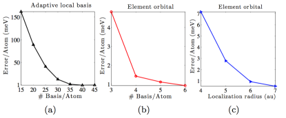
Figure 2: (color online) (a) Convergence of adaptive local basis functions (ALB) for a 3D bulk Na system with $432$ atoms. (b) Convergence of element orbitals (EO) for the same Na system with fixed number of ALBs. (c) Convergence in terms of the localization radius for the same Na system with fixed number of ALBs and fixed number of EOs.

Compared to ALB, the EO approach introduces an additional parameter which is the localization radius. Fig. 2 (c) shows the error of the total free energy per atom using $42$ ALBs per atom, and $6$ EOs per atom but with different localization radius. When the localization radius is $4.0$ a.u. which is $53\%$ the length of an element, the error of the total energy per atom is $7$ meV. Moderate choice of the localization radius of $6.0$ a.u. ($69\%$ of the length of an element) yields accuracy around $1$ meV per atom. Fig. 2 (c) shows that our method is stable even for a large localization radius $7.0$ a.u. ($92\%$ of the length of an element), and the error is even smaller and is below $1$ meV per atom. We also remark that if the localization radius is further increased, the EOs are no longer localized around the element, but become fully extended in the extended element. This can lead to an unstable scheme with large error. Fig. 2 (c) shows that the accuracy of the EO is not very sensitive to the choice of localization radius.

EOs can resemble atomic orbitals but with local modifications reflecting the environmental effect, despite the fact that they are constructed in the extended elements with rectangular domain. Using the same Na system as example, we show in Fig. 3 the isosurface of the first $9$ element orbitals ($\phi_{1}$ to $\phi_{9}$) belonging to the same extended element, with the red and blue color indicating the positive and negative part of the EOs, respectively. $27$ atoms nearest to these EOs within a sphere of radius $6.0$ a.u. are also plotted in Fig. 3 as gold balls. We see that $\phi_{1}$ mimics $s$ orbital, $\phi_{2}$-$\phi_{4}$ mimic $p$-orbitals, and $\phi_{5}$-$\phi_{9}$ mimic $d$-orbitals. Both the general shape and the multiplicity of the element orbitals agree well with the physical intuition. We also find that hybridization of the $s,p,d$ orbitals naturally appears in the EOs, reflecting the effect of the environment. For example, the isosurface of $\phi_{1}$ exhibits “holes” around atoms. These holes are not described in the spherical symmetric $s$ atomic orbital, but can only be reflected in orbitals of higher angular momentum such as $d$ orbitals. Therefore, EOs are natural generalization of atom-centered orbitals, with both the atomic and environmental effect taken into account simultaneously.

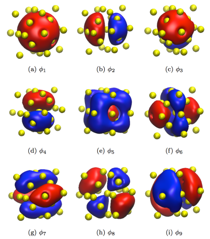
Figure 3: The isosurface of the first $9$ element orbitals belonging to the same extended element, for a 3D bulk Na system with $432$ atoms. The $27$ Na atoms nearest to the element orbitals within a sphere of radius $6.0$ a.u. are plotted as gold balls. The positive and negative part of the element orbitals are represented by red and blue color, respectively.

EOs are localized in the extended elements. Since each candidate function is not continuous across the boundary of the extended element, EOs are still discontinuous across the boundary of the extended element. Nonetheless, the EOs are “qualitatively continuous” at the boundary of the extended elements. Fig. 4 (a) shows the behavior of $\phi_{1},\phi_{4},\phi_{7}$ for the Na system along one $[100]$ direction, with the zoom-in near the boundary of the extended element shown in Fig. 4 (b). EOs are very close to a continuous function especially for $\phi_{1}$ and $\phi_{4}$ with lower angular momentum. The value of EOs of higher angular momentum such as $\phi_{7}$ at the grid point closest to the boundary of the extended element is within $10^{-3}$.

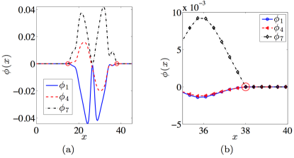
Figure 4: (color online) (a) The value of the element orbitals $\phi_{1}$ (blue solid line),$\phi_{4}$ (red dashed line), and $\phi_{7}$ (black dot dashed line) along one $[100]$ direction of a 3D bulk Na system with $432$ atoms. The two red circles indicate the boundary of the extended element. (b) Zoom-in of (a) to the region near the boundary of the extended element. The same set of element orbitals $\phi_{1}$ (blue solid line with circles), $\phi_{4}$ (red dashed line with triangles) and $\phi_{7}$ (black dot dashed line with diamonds) are shown, with the symbols indicating the position of the numerical grids. The red circle indicates the boundary of the extended element.

EOs can be used for calculating the relative energies of different atomic configurations. Fig. 5 (a) shows the total free energy per atom for a crystal of Na consisting of $6\times 6\times 6=216$ unit cells with $432$ atoms. Each unit cell is body centered cubic with $2$ Na atoms. The lattice constant ranges from $7.3$ a.u. to $7.9$ a.u.. The size of each element is equal to that of one unit cell. $4$ EOs per atom are constructed from $42$ ALBs per atom and are used for calculating the total free energy. The planewave cutoff for Kohn-Sham wavefunctions in ABINIT is $20$ Ry. The difference of the total energy per atom is less than $2$ meV across all the lattice constants. Similar result can be obtained for Si. The supercell for Si contains $4\times 4\times 4=64$ unit cells with $512$ atoms in total. Each unit cell is diamond cubic with $8$ Si atoms. Fig. 5 (b) reports the total free energy per atom for lattice constants from $9.9$ a.u. to $10.5$ a.u.. Each element only covers $\frac{2}{3}\times\frac{2}{3}\times\frac{2}{3}$ unit cells. We remark that elements occupying a fraction of the unit cell are allowed, which is important especially when EOs are applied to systems with defects and disorderedness. The planewave cutoff for Kohn-Sham wavefunctions in ABINIT is set to be $120$ Ry to achieve the high accuracy as benchmark solution. The localization radius is also $6.0$ a.u.. Starting from $50$ ALBs per atom, $10$ EOs per atom are computed. The difference of the total free energy per atom is less than $1$ meV for all lattice constants.

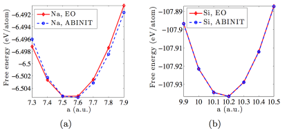
Figure 5: (color online) The total free energy per atom for 3D bulk Na system with $432$ atoms (a) and 3D bulk Si system with $512$ atoms (b), with different lattice constants calculated from ABINIT and from element orbitals.

EOs are also effective for calculating the total energy of systems with defects. For a crystal Na system with $432$ atoms and the length of each dimension of the supercell being $45.6$ a.u., the total free energy evaluated using ABINIT is $-103.27947$ a.u.. Using the same setup as done in the crystal system with $4$ EOs per atom, the total free energy evaluated using EO is $-103.27588$ a.u.. The difference is as small as $0.22$ meV per atom. Since our implementation takes the spin-unpolarized form, we consider a system with two vacancies by removing $2$ Na atoms belonging to one unit cell from the supercell. All the parameters are the same as those for the calculation of the crystal system. The total free energy evaluated using ABINIT is $-102.76957$ a.u., and the total free energy evalauted using $4$ EOs per atom is $-102.76637$ a.u., with the difference being $0.20$ meV per atom. The error for both the crystal and the defect system is less than $1$ meV per atom. We also estimate the formation energy of $M$ neutral vacancies by

$$\Delta E(M)=E^{d}_{N-M}-E^{0}_{N}\frac{N-M}{M},$$ (11)

with $E^{0}_{N}$ being the free energy for the crystal system with $N$ atoms, and $E^{d}_{N-M}$ being the free energy for the same system but with $M$ atoms removed. Atomic relaxation is not taken into account at this stage. Using (11), the formation energy calculated from ABINIT is $0.864$ eV, and that calculated from EO is $0.854$ eV. The difference of the formation energy is $0.010$ eV, and the relative error of the formation energy is $1.2\%$.

The calculation of the defect formation energy for Si is as follows. For a crystal Si system with $512$ atoms and the length of each dimension of the supercell being $40.4$ a.u., the total free energy evaluated using ABINIT is $-2030.85824$ a.u., and the total free energy evaluated using $10$ EOs per atom is $-2030.85691$ a.u.. The difference is as small as $0.07$ meV per atom. A defect system is constructed by removing one Si atom, and all the parameters are the same as those for the crystal calculation. The total free energy evaluated using ABINIT is $-2026.76478$ a.u., and the total free energy evaluated using $10$ EOs per atom is $2026.75974$ a.u., with the difference being $0.27$ meV per atom. The error for both the crystal system and that for the defect system is less than $1$ meV per atom. The formation energy calculated from ABINIT is $3.454$ eV, and that calculated from EO is $3.555$ eV. The difference of the formation energy is $0.101$ eV, and the relative error of the formation energy is $2.9\%$.

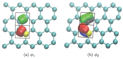
Figure 6: Graphene sheet consisting of $32$ C atoms (cyan balls) with $1$ C atom substituted by a Si atom (gold ball). Each black box represents an element. (a) The first element orbital $\phi_{1}$ (green) for the upper element with $2$ C atoms, and the first element orbital $\phi_{1}$ (red) for the lower element with $1$ C atom and $1$ Si atom. (b) The second element orbital $\phi_{2}$ (green for the positive part and black for the negative part) for the upper element with $2$ C atoms, and the second element orbital $\phi_{2}$ (red for the positive part and blue for the negative part) for the lower element with $1$ C atom and $1$ Si atom.

Next we study graphene sheet consisting of $32$ C atoms (cyan balls), with $1$ C atom replaced by a Si atom (gold ball), as shown in Fig. 6. The length of the supercell is $10.000$ a.u., $16.108$ a.u. and $18.600$ a.u. for $x,y,z$ directions, respectively. The C and Si atoms are in the $y-z$ plane. The supercell consists of $4\times 4$ elements, with each element containing $2$ atoms, and represented by one black box. The length of each element is therefore $10.00$ a.u., $4.027$ a.u. and $4.650$ a.u. along $x,y,z$ directions, respectively. The shape of the EOs is shown in Fig. 6 (a) for the first EOs $\phi_{1}$ belonging to $2$ different elements, and (b) for the second EOs $\phi_{2}$ belonging to the same $2$ elements, respectively. We find that $\phi_{1}$ in the upper element reflects the C-C bond and $\phi_{1}$ in the lower element reflects the C-Si bond, respectively. Similarly, $\phi_{2}$ reflects the $\pi$ bonds in both the upper and the lower elements. The shape of the EOs agree well with the physical intuition. In particular, the element orbitals are not centered around individual atoms but correspond directly to chemical bonds, which are of lower energy than individual atomic orbitals. Fig. 6 shows that the EOs constructed from a complete basis set such as planewaves provides a more flexible treatment of chemical environment than atom centered orbitals. The total free energy calculated using ABINIT with a planewave cutoff at $200$ Ry is $-180.56324$ a.u.. $12$ EOs per atom contracted from $40$ ALBs per atom with localization radius being $3.0$ a.u.. The total free energy calculated using EO is $-180.56279$ a.u.. The difference in the total free energy per atom is $0.38$ meV.

A more complicated example is a graphene sheet with $512$ C atoms, and with $128$ of the C atoms randomly selected and replaced by Si atoms. The atomic configuration is shown in Fig. 7 (a), with the C atoms represented by cyan balls and Si atoms represented by gold balls, respectively. The atoms are all in the $y-z$ plane, and the dimension of the supercell is $10.000$ a.u., $64.432$ a.u. and $74.400$ a.u. along $x,y,z$ directions, respectively. The electron density in the $y-z$ plane is shown in Fig. 7 (b). The total free energy calculated from ABINIT is $-2639.02487$ a.u., and the total free energy calculated from EO with $12$ EOs per atom for all elements is $-2639.11504$ a.u.. The error of the total free energy per atom is $4.79$ meV per atom.

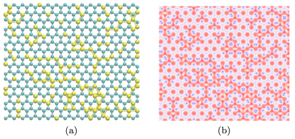
Figure 7: (a) The atomic configuration of a graphene sheet consisting of $512$ C atoms (cyan balls), with $128$ C atoms randomly selected and substituted by Si atoms (gold balls). (b) The electron density across $y-z$ plane.

The fact that a small number of EOs per atom already achieve high accuracy allows us to perform calculations for systems of large size. Here we study 3D bulk Na systems of various sizes, ranging from $128$ atoms to $4394$ atoms. The length of the supercell along each dimension is also proportional to the system size, from $30.4$ a.u. for $128$ atoms to $98.8$ a.u. for $4394$ atoms. The number of processors (computational cores) used is chosen to be proportional to the number of atoms, with $64$ processors used for $128$ atoms, and $2196$ processors used for $4392$ atoms. $4$ EOs per atom are constructed from $42$ ALBs per atom for all calculations. The total time per SCF iteration is shown in Fig. 8. We find that even though the number of atoms increase by a factor of $34$, the wall clock time only increases by less than $4$ times from $114$ sec for $128$ atoms to $413$ sec for $4394$ atoms. The small increase of the total wall clock time is because the time for solving the generalized eigenvalue problem (9), which is asymptotically the computationally dominating part, only takes less than $100$ sec even for system as large as $4392$ atoms, thanks to the small number of basis functions per atom allowed to be used in the calculation. The time for generating the ALBs using LOBPCG and the time for constructing the EOs from the ALBs are flat for all systems, since these steps are localized in each extended element and the computational cost is independent of the global system size. The overall time for solving the generalized eigenvalue problem (9) has not dominated the computational time for $4392$ atoms with a Hamiltonian matrix of size $17568$. However, the wall clock time for this part already scales quadratically with respect to the number of atoms. Since the number of processors scale linearly with respect to the system size, the overall time for solving the generalized eigenvalue problem scales cubically with respect to the system size, and will eventually dominate the overall running time for systems of larger size. The overhead of the DG calculation involves the assembly of the DG matrix $\mathsf{H}$, the construction of the Hamiltonian matrix $\mathsf{C}^{t}\mathsf{H}\mathsf{C}$ and the mass matrix $\mathsf{C}^{t}\mathsf{C}$ using parallel matrix-matrix multiplication, as well as the communication time. As alluded to earlier, the parallel matrix-matrix multiplication treats $\mathsf{C}$ and $\mathsf{H}$ as dense matrices in the current implementation. Therefore the asymptotic scaling of this part has the same asymptotic cubic scaling as solving the generalized eigenvalue problem. All the rest of the computational time (classified as “other time” in Fig. 8) mainly includes constructing the electron density using (10) in the global domain, solving the Kohn-Sham potential from the electron density, charge mixing as well as the extra data communication.

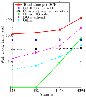
Figure 8: (color online) The total computational time per SCF iteration (red solid line with upward-pointing triangles) for 3D bulk Na systems ranging from $128$ atoms to $4394$ atoms. The breakdown of the total computational time includes the time for using LOBPCG to generate adaptive local basis functions (blue dashed line with diamonds), the time for constructing the element orbitals from adaptive local basis functions (black dot dashed line with circles), the time for solving the generalized eigenvalue problem using dense ScaLAPACK solver (green solid line with left-pointing triangles), the overhead time for solving the DG problem (magenta dashed line with right-pointing triangles), and the rest of the time in a SCF iteration (cyan dot dashed line with stars).

We also remark that treating the Hamiltonian matrix as dense matrices greatly increases the memory cost and the communication volume. Fig. 9 (a) shows the amount of memory used per processor. When the number of atoms is $4394$, the memory used per processor is $5.5$ GB, which becomes the bottleneck for further increasing the system size, despite that the computational time per SCF is still within affordable range. The communication volume, indicated by the percentage of the communication time within the total computational time is shown in Fig. 9 (b). The communication time occupies more than $40\%$ of the total time for systems with $4394$ atoms. Both the large memory cost and the large communication volume is largely due to the treatment of $\mathsf{C}$ and $\mathsf{H}$ as dense matrices, and shall be improved in the future work.

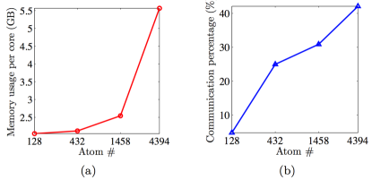
Figure 9: (color online) The memory cost per processor (a) and the communication percentage (b) for 3D bulk Na systems ranging from $128$ atoms to $4394$ atoms.

VI Conclusion

In conclusion, we have introduced the element orbitals for discretizing the Kohn-Sham Hamiltonian in the pseudopotential framework, which are contracted automatically from a uniform basis set. Comparing with the existing contracted basis sets, element orbitals incorporate environment information by including directly all atoms in the neighboring elements on the fly. The implementation of element orbitals is straightforward thanks to the rectangular partitioning of the domain. The accuracy of element orbitals are systematically improvable and the same procedure can be applied to systems under various conditions. The element orbitals are constructed by solving KSDFT locally in the real space, and localized on each element via a localization procedure. We remark that the localization procedure used for constructing the element orbitals is not grounded on the near-sightedness property as in the linear scaling methods for insulating systems Goedecker (1999); Kohn (1996). Instead of finding the compact representations for the Kohn-Sham invariant subspaces Gygi (2009), the current work seeks for a set of compact basis functions in the real space, while the coefficients of the basis set for representing the Kohn-Sham orbitals can still be delocalized. As is shown by the numerical examples, the current procedure is applicable to both insulating and metallic systems.

Our numerical examples also indicate that treating $\mathsf{C}$ and $\mathsf{H}$ as dense matrices can greatly increase the memory cost, the communication volume and the computational time especially for systems of large size. The future improvement includes treating $\mathsf{C}$ and $\mathsf{H}$ as sparse matrices so that the construction of the Hamiltonian matrix $\mathsf{C}^{t}\mathsf{H}\mathsf{C}$ and the mass matrix $\mathsf{C}^{t}\mathsf{C}$ is of linear scaling. By treating $\mathsf{C}$ and $\mathsf{H}$ as sparse matrices, we can also incorporate the recently developed pole expansion and selected inversion type fast algorithms Lin et al. (2009a, b, c, 2011a, 2011b, 2012b) to reduce the asymptotic scaling for solving the generalized eigenvalue problem (9) from cubic scaling to at most quadratic scaling for 3D bulk systems. We also remark that the current procedure for constructing the orbitals from adaptive local basis functions is still a costly procedure inside each element. Method for generating element orbitals directly inside the extended element is also under our exploration.

This work is partially supported by NSF CAREER Grant 0846501 (L. Y.), and by the Laboratory Directed Research and Development Program of Lawrence Berkeley National Laboratory under the U.S. Department of Energy contract number DE-AC02-05CH11231 (L. L.). The authors thank Jianfeng Lu for helpful discussions, and National Energy Research Scientific Computing Center (NERSC) for the support to perform the calculations. L. L. also thanks Weinan E for encouragement, and the University of Texas at Austin for the hospitality where the idea of this paper starts.

References

- Kohn and Sham (1965) W. Kohn and L. Sham, Phys. Rev. 140, A1133 (1965).
- Troullier and Martins (1991) N. Troullier and J. L. Martins, Phys. Rev. B 43, 1993 (1991).
- Vanderbilt (1990) D. Vanderbilt, Phys. Rev. B 41, 7892 (1990).
- Andersen (1975) O. K. Andersen, Phys. Rev. B 12, 3060 (1975).
- Blöchl (1994) P. E. Blöchl, Phys. Rev. B 50, 17953 (1994).
- Ozaki (2003) T. Ozaki, Phys. Rev. B 67, 155108 (2003).
- Blum et al. (2009) V. Blum, R. Gehrke, F. Hanke, P. Havu, V. Havu, X. Ren, K. Reuter, and M. Scheffler, Comput. Phys. Commun. 180, 2175 (2009).
- Junquera et al. (2001) J. Junquera, O. Paz, D. Sanchez-Portal, and E. Artacho, Phys. Rev. B 64, 235111 (2001).
- Chen et al. (2010) M. Chen, G. C. Guo, and L. He, J. Phys.: Condens. Matter 22, 445501 (2010).
- Andersen and Saha-Dasgupta (2000) O. K. Andersen and T. Saha-Dasgupta, Phys. Rev. B 62, R16219 (2000).
- Qian et al. (2008) X. Qian, J. Li, L. Qi, C. Z. Wang, T. L. Chan, Y. X. Yao, K. M. Ho, and S. Yip, Phys. Rev. B 78, 245112 (2008).
- Bowler and Miyazaki (2012) D. R. Bowler and T. Miyazaki, Rep. Prog. Phys. 75, 036503 (2012).
- Frisch et al. (1984) M. Frisch, J. Pople, and J. Binkley, J. Chem. Phys. 80, 3265 (1984).
- Clark et al. (1983) T. Clark, J. Chandrasekhar, G. Spitznagel, and P. Schleyer, J. Comput. Chem. 4, 294 (1983).
- Lin et al. (2012a) L. Lin, J. Lu, L. Ying, and W. E, J. Comput. Phys. 231, 2140 (2012a).
- Arnold (1982) D. N. Arnold, SIAM J. Numer. Anal. 19, 742 (1982).
- Gonze et al. (2009) X. Gonze, B. Amadon, P. Anglade, J. Beuken, F. Bottin, P. Boulanger, F. Bruneval, D. Caliste, R. Caracas, M. Cote, et al., Comput. Phys. Commun. 180, 2582 (2009).
- Rayson and Briddon (2009) M. J. Rayson and P. R. Briddon, Phys. Rev. B 80, 205104 (2009).
- Rayson (2010) M. J. Rayson, Comput. Phys. Commun. 181, 1051 (2010).
- Mermin (1965) N. Mermin, Phys. Rev. 137, A1441 (1965).
- Ceperley and Alder (1980) D. M. Ceperley and B. J. Alder, Phys. Rev. Lett. 45, 566 (1980).
- Perdew and Zunger (1981) J. P. Perdew and A. Zunger, Phys. Rev. B 23, 5048 (1981).
- Kleinman and Bylander (1982) L. Kleinman and D. M. Bylander, Phys. Rev. Lett. 48, 1425 (1982).
- Arnold et al. (2002) D. N. Arnold, F. Brezzi, B. Cockburn, and L. D. Marini, SIAM J. Numer. Anal. 39, 1749 (2002).
- Zhao et al. (2008) Z. Zhao, J. Meza, and L. Wang, J. Phys.: Condens. Matter 20, 294203 (2008).
- García-Cervera et al. (2009) C. J. García-Cervera, J. Lu, Y. Xuan, and W. E, Phys. Rev. B 79, 115110 (2009).
- Lin et al. (2009a) L. Lin, J. Lu, R. Car, and W. E, Phys. Rev. B 79, 115133 (2009a).
- Lin et al. (2009b) L. Lin, J. Lu, L. Ying, and W. E, Chin. Ann. Math. Ser. B 30, 729 (2009b).
- Lin et al. (2009c) L. Lin, J. Lu, L. Ying, R. Car, and W. E, Commun. Math. Sci. 7, 755 (2009c).
- Lin et al. (2011a) L. Lin, C. Yang, J. Lu, L. Ying, and W. E, SIAM J. Sci. Comput. 33, 1329 (2011a).
- Lin et al. (2011b) L. Lin, C. Yang, J. Meza, J. Lu, L. Ying, and W. E, ACM. Trans. Math. Software 37, 40 (2011b).
- Lin et al. (2012b) L. Lin, M. Chen, C. Yang, and L. He, arxiv:1202.2159 (2012b).
- Knyazev (2001) A. Knyazev, SIAM J. Sci. Comp. 23, 517 (2001).
- Teter et al. (1989) M. P. Teter, M. C. Payne, and D. C. Allan, Phys. Rev. B 40, 12255 (1989).
- Blackford et al. (1997) L. S. Blackford, J. Choi, A. Cleary, E. D’Azevedo, J. Demmel, I. Dhillon, J. Dongarra, S. Hammarling, G. Henry, A. Petitet, et al., ScaLAPACK Users’ Guide (SIAM, Philadelphia, PA, 1997).
- Hartwigsen et al. (1998) C. Hartwigsen, S. Goedecker, and J. Hutter, Phys. Rev. B 58, 3641 (1998).
- Pask and Sterne (2005) J. E. Pask and P. A. Sterne, Phys. Rev. B 71, 113101 (2005).
- Alavi et al. (1994) A. Alavi, J. Kohanoff, M. Parrinello, and D. Frenkel, Phys. Rev. Lett. 73, 2599 (1994).
- Anderson (1965) D. Anderson, J. Assoc. Comput. Mach. 12, 547 (1965).
- Kerker (1981) G. P. Kerker, Phys. Rev. B 23, 3082 (1981).
- Goedecker (1999) S. Goedecker, Rev. Mod. Phys. 71, 1085 (1999).
- Kohn (1996) W. Kohn, Phys. Rev. Lett. 76, 3168 (1996).
- Gygi (2009) F. Gygi, Phys. Rev. Lett. 102, 166406 (2009).