Quark lepton unification in higher dimensions

Abstract

The idea of unifying quarks and leptons in a gauge symmetry is very appealing. However, such an unification gives rise to leptoquark type gauge bosons for which current collider limits push their masses well beyond the TeV scale. We present a model in the framework of extra dimensions which breaks such quark-lepton unification symmetry via compactification at the TeV scale. These color triplet leptoquark gauge bosons, as well as the new quarks present in the model, can be produced at the LHC with distinctive final state signatures. These final state signals include high $p_{T}$ multi-jets and multi-leptons with missing energy, monojets with missing energy, as well as the heavy charged particles passing through the detectors, which we also discuss briefly. The model also has a neutral Standard Model singlet heavy lepton which is stable, and can be a possible candidate for the dark matter.

I Introduction

Unifying quarks and leptons in the same multiplet of a gauge symmetry group is very elegant, and answers naturally why the quarks have fractional charges while the leptons have integer charges. Such an unification has been achieved in the framework of partial unification in $SU(4)_{C}\times SU(2)_{L}\times SU(2)_{R}$  Pati:1974yy , or grand unification such as $SU(5)$ gg or $SO(10)$ gfm . The leptoquark gauge bosons present in such grand unification lead to proton decay which has not been observed so far, and pushes the mass scale of these leptoquark gauge bosons to $~{}10^{16}$ GeV. This is well beyond the reach of any present or future high energy collider. In the partial unification model, such as Pati-Salam type, since $B-L$ and the fermion number is conserved, there is no proton decay by the leptoquark gauge bosons. However, the leptoquark gauge boson here can cause rare meson decays, such as $K_{L}\rightarrow{\mu^{+}e^{-}}$ and $K_{L}\rightarrow{\mu^{-}e^{+}}$  Valencia:1994cj . The upper limit for the combined branching ratio for these two rare modes is $4.7\times 10^{-12}$ pdg . This gives the mass of the exchanged leptoquark gauge boson to be $>2.3\times{10^{3}}$ TeV. This is well above the current or future LHC reach. The question we address in this work is can we have a model in which the leptoquark gauge boson has a mass in the TeV scale which can be probed at the LHC?

One trick to achieve such a low scale for quark-lepton unification in the framework of $SU(4)_{C}$ is to pair the known quarks with some new leptons, and the known leptons with some new quarks. Then the leptoquark gauge bosons will couple known quarks with these new leptons, and the known leptons with new quarks. This will avoid the limits from the above flavor-violating rare meson decay limits, by choosing the mixing angles between the ordinary and new fermions small. But this will cause problems with the precision electroweak parameters, since these new fermions will be chiral and we are doubling chiral fermion sector of the Standard Model (SM).

However, such a scenario can be implemented by considering Pati-Salam type model in the framework of extra dimensions, say in five dimensions. Then upon orbifold compactification of the extra dimension, the zero modes of the new fermions can be projected out, leaving only the known quarks and leptons as the zero modes. The same orbifold compactification can be used to break the $SU(4)_{C}$ symmetry to $SU(3)_{C}$ and will give masses to the leptoquark gauge bosons at the compactification scale which can be chosen at a TeV. After compactification, in the four dimensional theory, the new fermions will have only Kaluza-Klein modes, and will be vector-like, thus avoiding any problem with the electroweak (EW) precision parameters. We will implement this scenario with the simplest Pati-Salam type model with the gauge symmetry $SU(4)_{C}\times U(1)_{I3R}\times SU(2)_{L}$ in five dimensions; and breaking the symmetry to $SU(3)_{C}\times SU(2)_{L}\times U(1)_{I3R}\times U(1)_{B-L}$ upon compactification to four dimensions. $U(1)_{I3R}\times U(1)_{B-L}$ will be broken down to $U(1)_{Y}$ using the usual Higgs mechanism. The leptoquark gauge bosons, as well as the new quarks (which will be the lightest KK excitations), with masses at the TeV scale can be produced at the LHC giving distinctive signals for new physics. We mention here that quark lepton unification using higher dimension has been considered by Adibzadeh and P. Q. Hung (hung, ), however their gauge symemmtry is different from ours, and there main objective was obtaining naturally light Dirac neutrino and fermion localization.

The paper is organized as follows. In section II, we discuss a five dimensional non-supersymmetric formulation of the model. In section III, we discuss the one loop radiative correction, and calculate the particle spectrum. The phenomenological implications of the model: the productions, decays, and the new physics signals are discussed in section IV. In section V, we give a five dimensional supersymmetric version of the model. Section VI contains our conclusions.

II A non-supersymmetric 5D model: Model and Formalism

Our gauge symmetry is $SU(4)_{C}\times SU(2)_{L}\times U(1)_{I3R}$ in five dimensions. The $SU(4)_{C}$ symmetry unifying quarks and leptons is broken down to $SU(3)_{C}\times U(1)_{B-L}$ by compactifying the extra dimension, $y$ on a $S^{1}/(Z_{2}\times Z^{\prime}_{2})$ orbifold. (The breaking of gauge symmetry via orbifold compactification is very elegant and has been extensively used in the literature to build realistic models kawa ; GAFF ; LHYN ; AHJMR ; LTJ1 ; Hall:2001tn ; Haba:2001ci ; Asaka:2001eh ; LTJ2 ; Dermisek:2001hp ; Li:2001tx ; Gogoladze:2003ci ; Gogoladze:2003yw ; Li:2003ee ). The remaining symmetry, $U(1)_{B-L}\times U(1)_{I3R}$ in our model in four dimensions (4D) is then broken down to the SM by using appropriate Higgs multiplets. All the particles, gauge bosons, Higgs bosons, as well as the fermions, propagate in the bulk, similar to the universal extra dimensions (UED)Appelquist:2000nn .

In the five-dimensional orbifold models the five-dimensional manifold is factorized into the product of ordinary four-dimensional Minkowski space-time $M^{4}$ and the orbifold $S^{1}/(Z_{2}\times Z^{\prime}_{2})$. The corresponding coordinates are $x^{\mu}$ ($\mu=0,1,2,3$) and $y\equiv x^{5}$. The radius for the fifth dimension is $R$. The orbifold $S^{1}/(Z_{2}\times Z^{\prime}_{2})$ is obtained by $S^{1}$ moduloing the equivalent class

$$P:~{}~{}y\sim-y~{},~{}P^{\prime}:~{}~{}y^{\prime}\sim-y^{\prime}~{},~{}\,$$ (1)

where $y^{\prime}\equiv y-\pi R/2$. There are two fixed points, $y=0$ and $y=\pi R/2$.

The gauge fields for $SU(4)_{C}\times SU(2)_{L}\times U(1)_{I3R}$ in five dimensions are $A4^{A}_{M}$, $A2^{A}_{M}$, and $A^{R}_{M}$, respectively, and $M=\mu,5$. All belong to the adjoint representations of the corresponding gauge symmetry. For generical five-dimensional gauge fields $A_{M}^{A}$, we have four-dimensional gauge fields $A_{\mu}^{A}$ and real scalar fields $A_{5}^{A}$. The fermion and Higgs representations in five dimensions have

$$FL_{L}~{}=~{}{\mathbf{(4,2,0)}}~{},~{}~{}FU_{R}~{}=~{}{\mathbf{(4,1,1/2)}}~{},~{}~{}FD_{R}~{}=~{}{\mathbf{(4,1,-1/2)}}~{}\,$$ (2)

and

$$FL^{{}^{\prime}}_{L}~{}=~{}{\mathbf{(4,2,0)}}~{},~{}~{}FU^{{}^{\prime}}_{R}~{}=~{}{\mathbf{(4,1,1/2)}}~{},~{}~{}FD^{{}^{\prime}}_{R}~{}=~{}{\mathbf{(4,1,-1/2)}}~{},~{}\,$$ (3)

$$H~{}=~{}{\mathbf{(1,1,-1/2)}}~{},~{}\,$$ (4)

where the numbers in the parentheses represent the quantum numbers with respect to the gauge symmetry, $SU(4)_{C}\times SU(2)_{L}\times U(1)_{I3R}$.

In the usual left and right handed notation, the particle contents in $FL$, $FL^{{}^{\prime}}$, $FU$, $FU^{{}^{\prime}}$, $FD$,$FD^{{}^{\prime}}$ are

$$FL_{L}=(q_{L},l^{{}^{\prime}}_{L}), FL_{R}=(q_{R},l^{{}^{\prime}}_{R}), FL^{{}^{\prime}}_{L}=(q^{{}^{\prime}}_{L},l_{L}), FL^{{}^{\prime}}_{R}=(q^{{}^{\prime}}_{R},l_{R}),$$

$$FU_{R}=(U_{R},N^{\prime}_{R}), FU_{L}=(U_{L},N^{{}^{\prime}}_{L}), FU^{{}^{\prime}}_{R}=(U^{{}^{\prime}}_{R},N_{R}), FU^{{}^{\prime}}_{L}=(U^{{}^{\prime}}_{L},N_{L}),$$

$$FD_{R}=(D_{R},E^{\prime}_{R}), FD_{L}=(D_{L},E^{{}^{\prime}}_{L}), FD^{{}^{\prime}}_{R}=(D^{{}^{\prime}}_{R},E_{R}), FD^{{}^{\prime}}_{L}=(D^{{}^{\prime}}_{L},E_{L}),$$ (5)

where we neglect the family indices $i=1,~{}2,~{}3$. These represent the fermions in one family. There are three such families. Note that the fermion content in each family has been quadrupled where $q_{L},l_{L},u_{R},d_{R},e_{R}$ and $N_{R}$ represent the usual fermions in a family (including a right-handed neutrino in each family), and the primes represent the additional fermions with same corresponding quantum numbers. Note that the leptoquark gauge bosons connect ordinary quarks to the exotic (primed) leptons, and ordinary leptons to exotic (primed) quarks. This will avoid the high experimental bound on the masses of these leptoquarks, and will allow us a low compactification scale for the $SU(4)_{C}\rightarrow SU(3)_{C}\times U(1)_{B-L}$ breaking.

We now discuss the gauge symmetry breaking via orbifold compactification, to break the $SU(4)_{C}$ gauge symmetry down to the $SU(3)_{C}\times U(1)_{B-L}$ gauge symmetry. Under the $Z_{2}$ and $Z^{\prime}_{2}$ parity operators $P$, and $P^{{}^{\prime}}$, the vector fields transform as

$$A_{\mu}(x^{\mu},y) \to A_{\mu}(x^{\mu},-y)=PA_{\mu}(x^{\mu},y)P^{-1}, A_{\mu}(x^{\mu},y^{{}^{\prime}}) \to A_{\mu}(x^{\mu},-y^{{}^{\prime}})=P^{{}^{\prime}}A_{\mu}(x^{\mu},y^{{}^{\prime}})P^{{}^{\prime}-1}$$

$$A_{5}(x^{\mu},y) \to A_{5}(x^{\mu},-y)=-PA_{5}(x^{\mu},y)P^{-1}, A_{5}(x^{\mu},y^{{}^{\prime}}) \to A_{5}(x^{\mu},-y^{{}^{\prime}})=-P^{{}^{\prime}}A_{5}(x^{\mu},y^{{}^{\prime}})P^{-1}$$ (6)

where $A_{5}$ is the $5$th component of the vector field.

The fermion multiplets belonging to the fundamental representation of the gauge symmetry transform as

$$Z_{2}:~{}~{}~{}~{}FL_{L}(x^{\mu},y) \to FL_{L}(x^{\mu},-y)=\eta PFL_{L}(x^{\mu},y)~{},$$

$$Z_{2}^{\prime}:~{}~{}~{}~{}FL_{L}(x^{\mu},y^{{}^{\prime}}) \to FL_{L}(x^{\mu},-y^{{}^{\prime}})=\eta P^{{}^{\prime}}FL_{L}(x^{\mu},y^{{}^{\prime}})~{},$$

$$Z_{2}:~{}~{}~{}~{}FL_{R}(x^{\mu},y) \to FL_{R}(x^{\mu},-y)=-\eta PFL_{R}(x^{\mu},y)~{},$$

$$Z_{2}^{\prime}:~{}~{}~{}~{}FL_{R}(x^{\mu},y^{{}^{\prime}}) \to FL_{R}(x^{\mu},-y^{{}^{\prime}})=-\eta P^{{}^{\prime}}FL_{R}(x^{\mu},y^{{}^{\prime}})$$ (7)

and similarly for the other fields. In a short-hand notation, the transformation properties of the fields are given by

$$FL_{L}:(\eta P,\eta P^{\prime}), FL_{R}:(-\eta P,-\eta P^{\prime}), FU_{R}:(\eta P,\eta P^{\prime}), FU_{L}:(-\eta P,-\eta P^{\prime}),$$

$$FD_{R}:(\eta P,\eta P^{\prime}), FD_{L}:(-\eta P,-\eta P^{\prime}), FL^{\prime}_{L}:(\eta P,-\eta P^{\prime}), FL^{\prime}_{R}:(-\eta P,\eta P^{\prime}),$$

$$FU^{\prime}_{R}:(\eta P,-\eta P^{\prime}), FU^{\prime}_{L}:(-\eta P,\eta P^{\prime}), FD^{\prime}_{R}:(\eta P,-\eta P^{\prime}), FD^{\prime}_{L}:(-\eta P,\eta P^{\prime})$$

where $\eta$ takes the value only $+1$.

To project out the zero modes of the fifth component of gauge fields, and the appropriate modes for the fermion fields, $FL$, and $FL^{{}^{\prime}}$ and others, we choose the following $4\times 4$ matrix representations for the parity operators $P$ and $P^{\prime}$

$$P={\rm diag}(+1,+1,+1,+1)~{},~{}P^{\prime}={\rm diag}(+1,+1,+1,-1)~{}.~{}\,$$ (8)

Under the $P^{\prime}$ parity, the gauge generators $T^{\alpha}$ ($\alpha=1$, $2$, …, $15$) for $SU(4)_{C}$ are separated into two sets: $T^{a}$ are the generators for the $SU(3)_{C}\times U(1)_{B-L}$ gauge group, and $T^{\hat{a}}$ are the generators for the broken gauge group

$$P~{}T^{a}~{}P^{-1}=T^{a}~{},~{}P~{}T^{\hat{a}}~{}P^{-1}=T^{\hat{a}}~{},~{}\,$$ (9)

$$P^{\prime}~{}T^{a}~{}P^{{}^{\prime}-1}=T^{a}~{},~{}P^{\prime}~{}T^{\hat{a}}~{}P^{{}^{\prime}-1}=-T^{\hat{a}}~{}.~{}\,$$ (10)

The zero modes of the $SU(4)_{C}/(SU(3)_{C}\times U(1)_{B-L})$ gauge bosons are projected out, thus, the five-dimensional $SU(4)_{C}$ gauge symmetry is broken down to the four-dimensional $SU(3)_{C}\times U(1)_{B-L}$ gauge symmetry. For the $SU(2)_{L}$ gauge symmetry, we choose

$$P~{}=~{}P^{\prime}~{}=~{}{\rm diag}(+1,+1)~{},~{}\,$$ (11)

and for the $U(1)_{R}$ gauge symmetry, we choose $P=P^{\prime}=1$. Thus, the $SU(2)_{L}\times U(1)_{I3R}$ remains unbroken after orbifold compactification.

Denoting the generical fields $\phi$ with parities ($P$, $P^{\prime}$)=($\pm,\pm$) by $\phi_{\pm\pm}$, we obtain the KK mode expansions

$$\phi_{++}(x^{\mu},y) = \sum_{n=0}^{\infty}\frac{1}{\sqrt{2^{\delta_{n,0}}\pi R}}\phi^{(2n)}_{++}(x^{\mu})\cos{2ny\over R}~{},~{}\,$$ (12)

$$\phi_{+-}(x^{\mu},y) = \sum_{n=0}^{\infty}\frac{1}{\sqrt{\pi R}}\phi^{(2n+1)}_{+-}(x^{\mu})\cos{(2n+1)y\over R}~{},~{}\,$$ (13)

$$\phi_{-+}(x^{\mu},y) = \sum_{n=0}^{\infty}\frac{1}{\sqrt{\pi R}}\,\phi^{(2n+1)}_{-+}(x^{\mu})\sin{(2n+1)y\over R}~{},~{}\,$$ (14)

$$\phi_{--}(x^{\mu},y) = \sum_{n=0}^{\infty}\frac{1}{\sqrt{\pi R}}\phi^{(2n+2)}_{--}(x^{\mu})\sin{(2n+2)y\over R}~{},~{}\,$$ (15)

where $n$ is a non-negative integer. The four-dimensional fields $\phi^{(2n)}_{++}$, $\phi^{(2n+1)}_{+-}$, $\phi^{(2n+1)}_{-+}$ and $\phi^{(2n+2)}_{--}$ acquire masses $2n/R$, $(2n+1)/R$, $(2n+1)/R$ and $(2n+2)/R$ upon the compactification. Zero modes are contained only in $\phi_{++}$ fields. Moreover, only $\phi_{++}$ and $\phi_{+-}$ fields have non-zero values at $y=0$, and only $\phi_{++}$ and $\phi_{-+}$ fields have non-zero values at $y=\pi R/2$.

$(P,P^{\prime})$	${\rm Field}$	${\rm Mass}$
$(+,+)$	$A4_{\mu}^{a}$, $A2_{\mu}^{A}$, $A^{R}_{\mu}$, $q_{L}$, $U_{R}$, $D_{R}$, $l_{L}$, $N_{R}$, $E_{R}$, $H$	${{2n}\over R}$
$(+,-)$	$A4_{\mu}^{\hat{a}}$, $q^{\prime}_{L}$, $U^{\prime}_{R}$, $D^{\prime}_{R}$, $l^{{}^{\prime}}_{L}$, $N^{\prime}_{R}$, $E^{\prime}_{R}$	${{2n+1}\over R}$
$(-,+)$	$A4^{\hat{a}}_{5}$, $q^{{}^{\prime}}_{R}$, $U^{{}^{\prime}}_{L}$, $D^{\prime}_{L}$, $l^{{}^{\prime}}_{R}$, $N^{\prime}_{L}$, $E^{\prime}_{L}$	${{2n+1}\over R}$
$(-,-)$	$A4_{5}^{a}$, $A2_{5}^{A}$, $A^{R}_{5}$, $q_{R}$, $U_{L}$, $D_{L}$, $L_{R}$, $N_{L}$, $E_{L}$,	${{2n+2}\over R}$

Table 1: Parity assignments and masses ($n\geq 0$) for the bulk fields.

The particle spectra and their $(P,~{}P^{\prime})$ parity are given in Table 5. Note that for each KK excitations, the left and right handed parts of each four-dimensional field combine to form a massive Dirac spinor.

The $SU(4)_{C}$ symmetry in our model is broken down to $SU(3)_{C}\times U(1)_{B-L}$ by the orbifold compactification $S^{1}/Z^{{}^{\prime}}_{2}$. To break the $U(1)_{B-L}\times U(1)_{I3R}$ gauge symmetry down to the $U(1)_{Y}$ gauge symmetry and give the Majorana masses to the right-handed neutrinos, we introduce a SM singlet Higgs field $S$ which is localized on the 3-brane at $y=\pi R/2$ and has a vacuum expectation value (VEV) at the TeV scale. The quantum number of $S$ under $SU(3)_{C}\times SU(2)_{L}\times U(1)_{B-L}\times U(1)_{I3R}$ gauge symmetry is $(\mathbf{1},\mathbf{1},\mathbf{-1},\mathbf{1})$. Finally, the $SU(2)_{L}\times U(1)_{Y}$ gauge symmetry breaking to $U(1)_{em}$ is achieved by using the usual standard model doublet Higgs $H$ with VEV at the electroweak scale. The complete SM fermion Yukawa couplings are

$$-{\cal L} = \left(\lambda^{u}_{ij}(FU^{j}_{R})^{c}FL^{i}_{L}\widetilde{H}+\lambda^{d}_{ij}(FD^{j}_{R})^{c}FL^{i}_{L}H+\lambda^{\prime u}_{ij}(FU^{\prime j}_{R})^{c}FL^{\prime i}_{L}\widetilde{H}+\lambda^{\prime d}_{ij}(FD^{\prime j}_{R})^{c}FL^{\prime i}_{L}H\right)$$ (16)

$$+\left(h^{u}_{ij}(FU^{j}_{R})^{c}FL^{i}_{L}\widetilde{H}+h^{d}_{ij}(FD^{j}_{R})^{c}FL^{i}_{L}H+h^{\prime u}_{ij}(FU^{\prime j}_{R})^{c}FL^{\prime i}_{L}\widetilde{H}+h^{\prime d}_{ij}(FD^{\prime j}_{R})^{c}FL^{\prime i}_{L}H\right)\delta(y)$$

$$+\left(y^{u}_{ij}(U_{R}^{j})^{c}q^{i}\widetilde{H}+y^{d}_{ij}(D_{R}^{j})^{c}q^{i}H+y^{\nu}_{ij}(N_{R}^{j})^{c}l^{i}_{L}\widetilde{H}+y^{e}_{ij}(E_{R}^{j})^{c}l^{i}_{L}H+y^{N}_{ij}S^{\dagger}N_{R}^{i}N_{R}^{j}\right)$$

$$\times\delta(y-\pi R/2)~{},~{}\,$$

where $\widetilde{H}=i\sigma_{2}H^{*}$ and $\sigma_{2}$ is the second Pauli matrix.

We define the $U(1)_{B-L}$ generator in $SU(4)_{C}$ as follows

$$T_{\rm U(1)_{B-L}}={\rm diag}\left({1\over 6},{1\over 6},{1\over 6},-{1\over 2}\right)~{}.~{}\,$$ (17)

Thus, we obtain the $U(1)_{B-L}$ gauge coupling $g_{B-L}$ and $SU(3)_{C}$ gauge coupling $g_{3}$ at the compactification scale in terms of $SU(4)_{C}$ gauge coupling $g_{4C}$

$$g_{B-L}~{}=~{}{\sqrt{3\over 2}}~{}g_{4C}~{},~{}~{}g_{3}=g_{4C}~{}.~{}\,$$ (18)

We denote the $U(1)_{Y}$ gauge field as $B_{\mu}$, and the orthogonal massive $U(1)$ gauge field as $Z^{\prime}_{\mu}$. Thus, we obtain

$$\left(\begin{array}[]{c}B_{\mu}\\ Z^{\prime}_{\mu}\end{array}\right)=\left(\begin{array}[]{cc}\cos\theta&\sin\theta\\ -\sin\theta&\cos\theta\end{array}\right)\left(\begin{array}[]{c}A_{\mu}^{R}\\ A_{\mu}^{B-L}\end{array}\right)~{},~{}\,$$ (25)

where

$$\sin\theta\equiv{{g_{R}}\over\displaystyle{\sqrt{g_{B-L}^{2}+g_{R}^{2}}}}~{},~{}\cos\theta\equiv{{g_{B-L}}\over\displaystyle{\sqrt{g_{B-L}^{2}+g_{R}^{2}}}}~{}.~{}\,$$ (26)

And the $Z^{\prime}_{\mu}$ mass is

$$M_{Z^{\prime}}~{}=~{}{\sqrt{2(g^{2}_{B-L}+g_{R}^{2})v^{2}}}~{}.~{}\,$$ (27)

Moreover, we obtain the $U(1)_{Y}$ gauge coupling as follows

$$g_{Y}^{2}={{g_{B-L}^{2}g_{R}^{2}}\over\displaystyle{g_{B-L}^{2}+g_{R}^{2}}}~{}.~{}\,$$ (28)

The covariant derivative for $B_{\mu}$ and $Z^{\prime}_{\mu}$ is

$$D_{\mu} \equiv \partial_{\mu}-iY_{B-L}g_{B-L}A_{\mu}^{B-L}-iY_{R}g_{R}A_{\mu}^{R}+\cdots$$ (29)

$$= \partial_{\mu}-ig_{Y}\left(YB_{\mu}+Y_{Z^{\prime}}Z^{\prime}_{\mu}\right)+\cdots~{},~{}\,$$

where $Y$ is the hypercharge, and

$$Y~{}=~{}Y_{B-L}+Y_{R}~{},~{}~{}~{}Y_{Z^{\prime}}~{}=~{}Y_{B-L}\cot\theta-Y_{R}\tan\theta~{}.~{}\,$$ (30)

When the $SU(4)_{C}$ gauge symmetry is broken down to the $SU(3)_{C}\times U(1)_{B-L}$ gauge symmetry, we can arrange the broken gauge fields into the vector fields $A^{\prime}_{\mu}$ and $\overline{A^{\prime}}_{\mu}$, whose quantum numbers under $SU(3)_{C}\times SU(2)_{L}\times U(1)_{Y}$ are $(\mathbf{3},\mathbf{1},\mathbf{2/3})$ and $(\mathbf{\overline{3}},\mathbf{1},\mathbf{-2/3})$. Their interactions with the matter fields can be obtained from the following covariant derivative

$$D_{\mu} \equiv \partial_{\mu}-i{{g_{4C}}\over{\sqrt{2}}}\left(\begin{array}[]{cc}G^{a}_{\mu}\lambda^{a}+A^{B-L}_{\mu}I_{3\times 3}/6&A^{\prime}_{\mu}\\ \overline{A^{\prime}}_{\mu}&-A^{B-L}_{\mu}/2\end{array}\right)+\cdots~{},~{}\,$$ (33)

where $G^{a}_{\mu}$ are the gluon fields, $\lambda^{a}$ are Gell-Mann matrices, and $I_{3\times 3}$ is the $3\times 3$ identity matrix.

III One loop radiative correction and particle spectrum

Note that in our model, first KK excitations of the the particles belonging to $(++)$ and $(--)$ have masses $2/R$, while those belonging to $(+-)$ and $(-+)$ have masses $1/R$. Thus at the tree level, all of the $(+-)$ and $(-+)$ are degenerate. However, radiative corrections will split these masses. The candidate for the dark matter, the decay pattern of these particles and the associated collider phenomenology will depend crucially on these radiative splittings.

The radiative corrections to the KK particle masses have not been calculated for the models on $S^{1}/(Z_{2}\times Z^{\prime}_{2})$. To have some idea about radiative corrections, we consider the $SU(4)_{C}\times SU(2)_{L}\times U(1)_{B-L}$ model on $S^{1}/Z_{2}$, i.e., we do not break the $SU(4)_{C}$ gauge symmetry via $Z_{2}$ orbifold projections. Using the generic formulae for radiative corrections given in Ref. Cheng:2002iz , we obtain the bulk radiative corrections to the KK particle masses

$$\delta\,(m_{A_{n}^{R}}^{2}) = -\frac{47}{2}\,\frac{g_{R}^{2}\,\zeta(3)}{16\pi^{4}}\left(\frac{1}{R}\right)^{2},$$

$$\delta\,(m_{W_{n}}^{2}) = -\frac{17}{2}\,\frac{g_{2}^{2}\,\zeta(3)}{16\pi^{4}}\left(\frac{1}{R}\right)^{2},$$

$$\delta\,(m_{A4_{n}}^{2}) = -6\,\frac{g_{4C}^{2}\,\zeta(3)}{16\pi^{4}}\left(\frac{1}{R}\right)^{2},$$

$$\delta(m_{F_{Ln}}) = \delta(m_{FU_{R}n})~{}=~{}\delta(m_{FD_{R}n})~{}=~{}\delta(m_{H_{n}}^{2})~{}=~{}0~{},~{}\,$$ (34)

where $\zeta(3)$ is about 1.202.

The boundary terms receive divergent contributions that require counter terms. The finite parts of these counter terms are undetermined and remain as free parameters of the theory. Assuming that the boundary kinetic terms vanish at the cutoff scale $\Lambda$ and calculate their renormalization to the lower energy scale $\mu$, we obtain the radiative corrections from the boundary terms

$$\bar{\delta}\,(m_{A^{R}_{n}}^{2}) = m_{n}^{2}\,\left(-\frac{1}{6}\right)\,\frac{g_{R}^{2}}{16\pi^{2}}\ln\frac{\Lambda^{2}}{\mu^{2}},$$

$$\bar{\delta}\,(m_{W_{n}}^{2}) = m_{n}^{2}\,\frac{15}{2}\,\frac{g_{2}^{2}}{16\pi^{2}}\ln\frac{\Lambda^{2}}{\mu^{2}},$$

$$\bar{\delta}\,(m_{A4_{n}}^{2}) = m_{n}^{2}\,\frac{46}{3}\,\frac{g_{4C}^{2}}{16\pi^{2}}\ln\frac{\Lambda^{2}}{\mu^{2}},$$

$$\bar{\delta}\,m_{FLn} = m_{n}\,\left(\frac{135}{32}\,\frac{g_{4C}^{2}}{16\pi^{2}}+\frac{27}{16}\,\frac{g_{2}^{2}}{16\pi^{2}}\right)\,\ln\frac{\Lambda^{2}}{\mu^{2}},$$

$$\bar{\delta}\,m_{FUn} = \bar{\delta}\,m_{FDn}~{}=~{}m_{n}\,\left(\frac{135}{32}\,\frac{g_{4C}^{2}}{16\pi^{2}}+\frac{9}{16}\,\frac{g_{R}^{2}}{16\pi^{2}}\right)\,\ln\frac{\Lambda^{2}}{\mu^{2}},$$

$$\bar{\delta}\,(m_{H_{n}}^{2}) = m_{n}^{2}\,\left(\frac{3}{2}\,g_{2}^{2}+\frac{3}{4}\,g_{R}^{2}-\lambda_{H}\right)\frac{1}{16\pi^{2}}\ln\frac{\Lambda^{2}}{\mu^{2}}+\overline{m}_{H}^{2}~{},~{}\,$$ (35)

where $\lambda_{H}$ is the Higgs quartic coupling (${\cal L}\supset-(\lambda_{H}/2)(H^{\dagger}H)^{2}$), and $\overline{m}_{H}^{2}$ is the boundary Higgs mass term. The renormalization scale $\mu$ should be taken to be approximately the mass of the corresponding KK mode. For simplicity, we neglect the Yukawa coupling corrections here since their corrections are about one or two percents even for order one Yukawa couplings. Thus, comparing to the boundary corrections, the bulk corrections to the $SU(4)_{C}\times SU(2)_{L}$ gauge bosons’ masses are indeed very small since in addition to the coefficients, there is another $\pi^{2}$ suppressions. However, for $U(1)_{R}$ gauge boson, the bulk corrections are larger than the boundary corrections. In addition, the boundary corrections to $SU(4)_{C}$ gauge bosons’ masses are much larger than those to the $FL$, $\overline{FU}$ and $\overline{FD}$.

Figure 1: The particle mass spectrum of the $(+-)$ states for two values of the compactification scale $R$ after including the mass splittings.

The gauge symmetry $SU(4)_{C}$ is broken down to $SU(3)_{C}\times U(1)_{B-L}$ by the orbifold compactification $S^{1}/Z^{{}^{\prime}}_{2}$. The $SU(3)$ color interaction will split the masses among the members of the $(+-)$ modes. We estimate these splittings as

$$\bar{\delta}\,m_{q^{{}^{\prime}}_{Ln}}-\bar{\delta}\,m_{l^{{}^{\prime}}_{Ln}} = m_{n}\,3\frac{g_{3C}^{2}}{16\pi^{2}}\ln\frac{\Lambda^{2}}{\mu^{2}},$$ (36)

$$\bar{\delta}\,m_{u^{{}^{\prime}}_{Rn}}-\bar{\delta}\,m_{N^{{}^{\prime}}_{Rn}} = m_{n}\,\frac{3g_{3C}^{2}+g^{\prime 2}}{16\pi^{2}}\ln\frac{\Lambda^{2}}{\mu^{2}},$$ (37)

$$\bar{\delta}\,m_{d^{{}^{\prime}}_{Rn}}-\bar{\delta}\,m_{E^{{}^{\prime}}_{Rn}} = m_{n}\,\frac{3g_{3C}^{2}-2g^{\prime 2}}{16\pi^{2}}\ln\frac{\Lambda^{2}}{\mu^{2}},$$ (38)

where

$$\bar{\delta}\,m_{q^{{}^{\prime}}_{Ln}}=\delta(m_{FLn}), \bar{\delta}\,m_{u^{{}^{\prime}}_{Rn}}=\delta(m_{FURn}), \bar{\delta}\,m_{d^{{}^{\prime}}_{Rn}}=\delta(m_{FDRn}),$$ (39)

the expressions for which are given before. Using the above equations, the spectrum of the first KK excitations of the particles can be calculated. Two parameters in the model are $1/R$ and $\Lambda$. In Fig. 1, we have shown the particle spectrum for $1/R=400$ GeV, $\Lambda R=20$, and for $1/R=600$ GeV, and $\Lambda R=20$. We also list the explicit values of the masses in Table 2.

After calculating the mass splittings, the heaviest state in the particle spectrum for the first KK excited states with parity properties $(+-)$ turns out to be the fractionally charged colored vector boson $A^{\prime}$. The colored fermion states are much heavier than the lepton excitations and the lowest lying particles in the mass spectrum are the neutral $SU(2)_{L}$ and color singlet excitation ($N^{\prime}$) of the right-handed neutrino, which we call as the lightest exotic particle (LXP). In Fig. 2 we show the mass of the KK excitations as a function of the compactification scale $R^{-1}$. The larger values of the compactification scale lead to larger mass splittings between the different particles.

Just like any other model with some discrete parity symmetry preventing the decay of the lightest particle into only SM particles, the LXP in our model ($N^{\prime}$) too is stable and a candidate for cold dark matter.

Particles	$A^{\prime}$	$q^{{}^{\prime}i}$	$U^{{}^{\prime}i}$	$D^{{}^{\prime}i}$	$l^{{}^{\prime}i}$	$E^{{}^{\prime}i}$	$N^{{}^{\prime}i}$
$R^{-1}=400$	544.5	505.5	495.8	495.8	438.2	432.4	426.6
$R^{-1}=600$	816.7	758.2	743.7	743.7	657.3	648.6	639.9

Table 2: The masses (in GeV) for the KK excitations of the $(+-)$ states for two values of the compactification scale $R$ where $\Lambda R=20$.

Figure 2: The particle mass spectrum as a function of the compactification scale $R^{-1}$ after including the mass splittings.

IV Phenomenological Implications: Decay modes and collider signals

By construction one expects the phenomenology of this model to have features present in the UED type models (for example, see uedmodels , where one produces the KK excitations of the SM particles and studies the multi-lepton and multi-jet final states accompanied with a large missing energy carried away by the lightest KK particle. However, the motivation of our model is completely different, namely, the quark lepton unification. Thus our model has leptoquark gauge bosons, as well as new fermions not present in the UED type models. Also, in our model, the first KK excitations of the SM particles are much heavier with the mass scale of $2/R$, instead of $1/R$, whereas the KK excitations of the new particles ($q^{\prime},l^{\prime}$) have mass scale of $1/R$. These particles are not present in the UED type models. The interesting signal in our model arises from the production of the KK excitations of the new strongly interacting exotic fermions ($q^{\prime},U^{\prime},D^{\prime}$) as well as the KK excitations of the colored leptoquark gauge boson ($A^{\prime}$). All these modes have large pair production cross sections as their production proceeds through strong interactions. In Fig. 3 we plot the pair production cross sections for the strongly interacting exotics as well as the leptonic modes at LHC for two different center of mass energies $7$ and $14$ TeV.

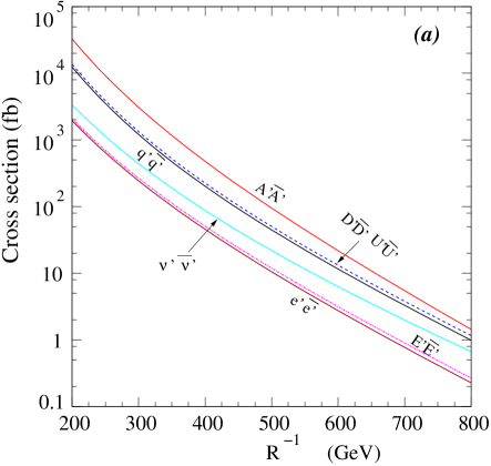
Figure 3: Illustrating the pair production cross sections for the first KK excitations as a function of the compactification scale $R^{-1}$ at LHC for the center-of-mass energies of (a) $\sqrt{s}=7$ TeV and (b) $\sqrt{s}=14$ TeV.

It is worth noting that the fractionally charged vector boson $A^{\prime}$ has the largest production cross section at the LHC and it couples directly to the gluon with the interaction vertices ($G~{}A^{\prime}~{}A^{\prime}$) and ($G~{}G~{}A^{\prime}~{}A^{\prime}$). Also, it mediates the decay of the exotic fermions. The decay of these exotics determine the phenomenological implications of this model at collider experiments. To highlight the interesting signal this model has at colliders, we look at all the possible decay modes that these exotics have for the two values of $R^{-1}=400$ GeV and $R^{-1}=600$ GeV. The dominant decay channels along with their branching ratios are collected in Table 3, which we have calculated using CalcHEP Pukhov:2004ca .

Decay Modes	$R^{-1}=400$ GeV	$R^{-1}=600$ GeV	i
BR ($A^{\prime}\to\bar{e}^{i}D^{{}^{\prime}i}_{R}$)	2.03 %	1.99 %	1,2,3
BR ($A^{\prime}\to\nu_{L}^{i}u^{{}^{\prime}i}_{L}$)	1.34 %	1.31 %	1,2,3
BR ($A^{\prime}\to\bar{e}^{i}d^{{}^{\prime}i}_{L}$)	1.34 %	1.31 %	1,2,3
BR ($A^{\prime}\to d^{i}\bar{E}^{{}^{\prime}i}_{R}$)	8.81 %	8.64 %	1,2,3
BR ($A^{\prime}\to d^{i}\bar{e}^{{}^{\prime}i}_{L}$)	8.06 %	7.91 %	1,2,3
BR ($A^{\prime}\to u^{i}\nu^{{}^{\prime}i}_{L}$)	8.06 %	7.91 %	1,2
BR ($A^{\prime}\to u^{i}N^{{}^{\prime}i}_{R}$)	9.57 %	9.38 %	1,2
BR ($A^{\prime}\to tN^{{}^{\prime}3}_{R}$)	–	1.94 %
BR ($q^{{}^{\prime}1}_{L}\to\nu_{L}^{i}d^{i}\bar{E}^{{}^{\prime}i}_{R}$)	10.8 %	10.8 %	1,2,3
BR ($q^{{}^{\prime}1}_{L}\to\nu_{L}^{i}d^{i}\bar{e}^{{}^{\prime}i}_{L}$)	7.7 %	7.7 %	1,2,3
BR ($q^{{}^{\prime}1}_{L}\to\nu_{L}^{i}u^{i}\nu^{{}^{\prime}i}_{L}$)	7.7 %	7.7 %	1,2
BR ($q^{{}^{\prime}1}_{L}\to\nu_{L}^{i}u^{i}N^{{}^{\prime}i}_{R}$)	14.6 %	14.6 %	1,2
BR ($D^{{}^{\prime}1}_{R}\to ed^{i}\bar{E}^{{}^{\prime}i}_{R}$)	10.9 %	10.9 %	1,2,3
BR ($D^{{}^{\prime}1}_{R}\to ed^{i}\bar{e}^{{}^{\prime}i}_{L}$)	7.3 %	7.3 %	1,2,3
BR ($D^{{}^{\prime}1}_{R}\to eu^{i}\nu^{{}^{\prime}i}_{L}$)	7.3 %	7.3 %	1,2,3
BR ($D^{{}^{\prime}1}_{R}\to eu^{i}N^{{}^{\prime}i}_{R}$)	15.6 %	15.6 %	1,2
BR ($\nu^{{}^{\prime}1}_{L}\to u\bar{u}^{i}N^{{}^{\prime}i}_{R}$)	50 %	49 %	1,2
BR ($e^{{}^{\prime}1}_{L}\to\bar{u}dN^{{}^{\prime}1}_{R}$)	49.5 %	48.6 %
BR ($e^{{}^{\prime}1}_{L}\to\bar{c}dN^{{}^{\prime}2}_{R}$)	47.1 %	47.6 %
BR ($E^{{}^{\prime}1}_{R}\to\bar{u}dN^{{}^{\prime}1}_{R}$)	55.0 %	52.3 %
BR ($E^{{}^{\prime}1}_{R}\to\bar{c}dN^{{}^{\prime}2}_{R}$)	45.0 %	47.7 %

Table 3: The dominant decay modes and the respective branching ratios for the first KK excitation of the new exotic particles for two values of the compactification scale.

From Table 3, we note that the dominant decay channel for the leptoquark gauge boson, $A^{\prime}$ is to a light jet and the lightest KK particle, $N^{\prime}$ (around 10%). This would mean that the dominant signal in this case becomes 2 jets with large missing energy. The other dominant decay channels are $A^{\prime}\to d^{i}\bar{E}^{{}^{\prime}i}_{R};~{}d^{i}\bar{e}^{{}^{\prime}i}_{L}$ and $A^{\prime}\to u^{i}\nu^{{}^{\prime}i}_{L}$. However all the subsequent decay of the above exotics lead to multi-jet final states with a large amount of missing energy carried away by the LXP, $N^{\prime}$. It is worth noting that all decays other than that of $A^{\prime}$ are three-body decays since they all decay via $A^{\prime}$ exchange. Since the mass difference between the exotic quarks and the exotic leptons is quite large, the jets and leptons coming from the exotic quark decays would be much harder as compared to the jets that come from the exotic leptons. Thus even though one expects a high jet multiplicity in the signal, the sub-leading jets coming from decays of $e^{\prime},\nu^{\prime}$ and $E^{\prime}$ would be quite soft. Although a large jet multiplicity is nothing new at a hadron machine like the LHC, we must note that all the new exotics would finally decay to the LXP ($N^{\prime}$). Thus, along with a large jet multiplicity in the signal for the new exotics one needs to trigger on the final configuration demanding a large amount of missing energy which would very clearly be able to suppress the SM background without affecting the signal too much. One can also have multi-lepton final states but with lower signal events because of the smaller branching fractions as shown in Table 3. We must however note that the missing transverse energy ($\not{E}_{T}$) for our signal crucially depends on the mass splittings ($\Delta M$) between the LXP ($N^{\prime}$) and the heavy exotic it comes from. A small mass splitting would lead to smaller $\not{E}_{T}$ even for a heavy LXP as it would carry away very small kinetic energy. The exact behavior of the signal would require a detail simulation of the events in the hadronic collider environment which we leave for future studies.

	$R^{-1}=400$ GeV	$R^{-1}=600$ GeV
Signal	$\sigma\times BR$ (fb)	$\sigma\times BR$ (fb)
2 hard jets and $\not{E}_{T}$	8330	787
4 hard jets and $\not{E}_{T}$	611	53.6
1 lepton, 3 hard jets and $\not{E}_{T}$	1890	102
2 leptons, 2 hard jets and $\not{E}_{T}$	5020	393
2 leptons, 4 hard jets and $\not{E}_{T}$	30.0	2.75
4 leptons, 2 hard jets and $\not{E}_{T}$	30.0	2.75
Monojet ($p_{T}^{j}>20$ GeV) and $\not{E}_{T}$	2000	215

Table 4: Illustrating the $\sigma\times BR$ for the various final states obtained for the signal from the production and decay of the exotics at LHC with center-of-mass energy $\sqrt{s}=14$ TeV. The leptons considered in the final states are either $e$ or $\mu$.

The various important collider signatures are summarized in Table 4. We also give the $\sigma\times\mathrm{branching~{}ratio(BR)}$ for the different final state topologies which highlight the important signatures of our model. All the leptons are either $e$ or $\mu$ while the $\tau$’s have been considered as jets. No cuts have been made on the signal although we expect the basic acceptance cuts to reduce the signal by only 10%-20%. Note that the numbers shown are for a center-of-mass energy of $\sqrt{s}=14$ TeV at LHC. The corresponding numbers for the current center-of-mass energy of $\sqrt{s}=7$ TeV at which the LHC is running can be obtained by a simple scaling of the $\sigma\times~{}BR$ given in Table 4. The approximate scaling factors for $R^{-1}=400$ GeV and $R^{-1}=600$ GeV are $0.1$ and $0.05$ respectively. This implies that some of the final states listed might be difficult to observe in the current run of LHC but will have much higher and observable rates when the machine runs at a higher center-of-mass energy.

The signature common to all signals is a substantial amount of $\not{E}_{T}$ because of the undetected $N^{\prime}$ and neutrinos present in the final states, coming from the decay chains shown in Table 3. The leptonic signals primarily come from the decay of the $A^{\prime}$ and the $D_{R}^{\prime}$ exotics and give relatively large signal rates for the final state configurations of $1\ell+3j+\not{E}_{T}$ and $2\ell+2j+\not{E}_{T}$. The 4-lepton signature with at least 2 hard jets also looks very promising because of the very small SM background expected for such a signal. In addition, the model has large cross section for the monojet plus large $\not{E}_{T}$ signal. Each jet is considered hard if it’s $p_{T}>40$ GeV. We discuss the individual signals and the possible SM backgrounds below.

$n$ hard jets and $\not{E}_{T}$

Hadronic signals with missing $\not{E}_{T}$ appear with very large cross section in our model. However such signals are hard to analyze at a hadronic machine, unless the associated missing transverse energy is very big. With the mass splittings in our model not very big, we do not expect a very extravagant value for the $\not{E}_{T}$. There has been recent interest in looking for new physics signals in dijet events by using a kinematic variable

$$\alpha_{T}=\frac{p_{T}^{j_{2}}}{M_{jj}}$$ (40)

which was presented to study SUSY signatures of similar topology in the final state Randall:2008rw . The $p_{T}^{j_{2}}$ is the transverse momenta of the second leading jet while the $M_{jj}$ is the invariant mass of the dijet pair. The SM background trails off at 0.5 for back-to-back jets in QCD events and thus can help in looking for new physics signals which give large $\not{E}_{T}$ in the final state. This analysis has also been extended to final states with more than 2 jets Ozturk:2009fj . In addition one might require more specific set of selection cuts to isolate signals for new physics in final states with only jets and large missing transverse momenta Alves:2011sq . These techniques would also be useful in isolating our signal with $2j+\not{E}_{T}$ and $4j+\not{E}_{T}$ from the SM background.

1 lepton, 3 hard jets and $\not{E}_{T}$

The signal shown in Table 4 is for LHC running with the center-of-mass energy of 14 TeV. Without kinematic cuts the signal looks very promising. However, one expects several SM processes to give a similar final state. The most likely backgrounds to this process are $t\bar{t},~{}tW,~{}t\bar{t}Z,~{}WZ$ and $Wjj$ where one of the top quark decays semileptonically for the $t\bar{t}$ events, while either the top or $W$ gives the hard lepton for the $tW$ process, whereas the $W$ gives the lepton for the $WZ$ and $Wjj$ process. The backgrounds coming from the top quark processes can be suppressed using a $b$-jet veto on the signal, as our signal will only consist of the light quark jets. As we demand that the final state has at least 3 hard jets, the $WZ$ and $Wjj$ will have to have one additional jet from radiations which should suppress this background significantly. The single top SM background cross section is weak process and the cross section should be smaller and the strong selection cuts on the lepton, jets and the missing transverse energy should be enough to suppress this background. Similar weak process backgrounds like the triple gauge boson production should also give much smaller rates compared to the signal.

2 leptons, 2 hard jets and $\not{E}_{T}$

This process has a large $\sigma\times BR\simeq 500$ fb for $R^{-1}=400$ GeV at the current LHC energy. In addition the signal should be decently clean with 2 hard leptons in the final state. The potentially dominant SM background comes from $t\bar{t}$ process with some contributions from $t\bar{t}Z$ and other weak processes like the $WWW,~{}WWZ$. The background from pair production of tops will be very large at both $\sqrt{s}=7$ TeV and $\sqrt{s}=14$ TeV center-of-mass energy at LHC but can be again suppressed by using a $b$-jet veto on the signal. In our model we have hard jets that are equally likely to be u, c, s, d, or b. This signal is promising but a full analysis of the SM background needs to be done to know whether the signal can stand out over the background.

4 leptons, 2 hard jets and $\not{E}_{T}$

The 4-lepton signal is very clean and promising as very few SM processes can lead to such final states with appreciable cross section. However, we do find a low $\sigma\times BR=30$ fb when compared to the other final states listed in Table 4. With the available mass splitting for $R^{-1}=400$ GeV, we expect the leptons to have at least $p_{T}>30$ GeV. With 4 such hard leptons, 2 hard jets and substantial $\not{E}_{T}$, this signal should stand out over the negligible SM background. The most likely sources for the SM background are again $t\bar{t}$ and triple or four vector boson processes, where the additional leptons in the $t\bar{t}$ process coming from the decays of the b-quarks. The strong $p_{T}$ cut on the leptons and the additional requirement of 2 hard jets should make these background completely negligible. With high enough luminosity, even higher values of $R^{-1}$ could be probed through this signal.

The multi-lepton signals with large jet multiplicity also leads to interesting correlations in the signature space with that of the parameters of the theory for different new physics models beyond the SM and can be a useful way of distinguishing signatures in our model with other models with similar signatures Bhattacherjee:2009jh .

Monojet and $\not{E}_{T}$

In our model this signal is dominantly produced in the process, $pp\rightarrow N^{\prime}N^{\prime}g$. It is a signal with a single jet plus missing $E_{T}$ with balancing transverse momenta, at the LHC. The $\sigma\times BR$ for this mode is around 2 pb where the jet has a minimum $p_{T}$ cut of 20 GeV. The dominant SM background here comes from $Z+j$ in the hard $E_{T}$ regime where the Z decays invisibly while in the low $E_{T}$ regime it is dominated by QCD with mis-measurement of jets Vacavant:2001sd ; Rizzo:2008fp . As the single jet recoils against a massive system consisting of two heavy stable particles, it is expected to carry away a large transverse momenta which is balanced by the missing $E_{T}$. Thus a very high $\not{E}_{T}$ cut would make the signal significant against the large SM background dominated by the $Z+j$ process. Another interesting signature would be the single photon signature much similar to the monojet signal, with smaller signal rates.

A very long-lived colored charged particle

A very interesting prediction in our model is the presence of a long-lived charged colored exotic fermion ($U^{\prime}$). This particle is not listed in Table 4 with the branching probabilities of the various exotics. Because of the parity assignment of the particle content in our model, we find that the $U^{\prime}$ becomes very long lived and does not decay within the detector. Since it has to decay through the $A^{\prime}$ or the $A4_{5}^{\hat{a}}$ and the right-handed neutrino, it can only decay to a 5-body final state allowed by the kinematic phase space. The heavy right-handed neutrino gets a Majorana mass at the TeV scale through the VEV of the singlet scalar $S$ which breaks the additional U(1) symmetry. Assuming a TeV-seesaw mechanism to be responsible for the light neutrino masses in the SM, the Dirac Yukawa couplings are of the order of $10^{-6}$. This would also be the strength of the mixing angle between the heavy singlet right-handed neutrino and the light neutrinos. Thus the $U_{R}^{\prime}$ decays for example through the following decay chain:

$$U_{R}^{\prime}\to A^{\prime*}N_{R}^{*}\to(uN^{\prime})(e(W^{*}\to u\bar{d}))$$

Thus summing over all possible 5-body decays, we find that the width $\Gamma(U^{\prime})\sim 10^{-27}$ GeV which gives a rough lifetime of 100 seconds. Thus it cannot decay within the detector. However, being a colored particle it would hadronize quickly to form charged or neutral hadrons that would interact and pass through the detector Kraan:2004tz . Such scenarios can also happen in supersymmetric theories which have long-lived squarks, long-lived gluinos Giudice:2004tc ; ArkaniHamed:2004yi which form these type of hadrons. The neutral hadron would usually pass through the detector undetected, while the charged hadron would be slow moving highly ionizing particle leaving a charged track in the muon detector and passing through Drees:1990yw ; Fairbairn:2006gg . Thus one can have 1 or 2 heavily ionizing charged tracks in the detector passing through the muon chamber. Being a colored particle, the pair production cross section for the $U_{R}^{\prime}$ is quite large, as shown in Fig. 3. Such a signature will be a unique test of our model, complemented with the other signals listed above and also distinguishes our model from all other beyond SM theories. There are already strong constraints on such particles from the LHC experiments Khachatryan:2011ts ; Aad:2011hz .

V A Five-Dimensional Supersymmetric Model

In this Section, we shall also construct the five-dimensional $N=1$ supersymmetric $SU(4)_{C}\times SU(2)_{L}\times U(1)_{I3R}$ models on $S^{1}/(Z_{2}\times Z^{\prime}_{2})$. The $N=1$ supersymmetric theory in five dimensions have 8 real supercharges, corresponding to $N=2$ supersymmetry in four dimensions. In terms of the physical degrees of freedom, the vector multiplet contains a vector boson $A_{M}$ with $M=0,1,2,3,5$, two Weyl gauginos $\lambda_{1,2}$, and a real scalar $\sigma$. In the four-dimensional $N=1$ supersymmetry language, it contains a vector multiplet $V\equiv(A_{\mu},\lambda_{1})$ and a chiral multiplet $\Sigma\equiv((\sigma+iA_{5})/\sqrt{2},\lambda_{2})$ which transform in the adjoint representation of group $G$. The five-dimensional hypermultiplet consists of two complex scalars $\phi$ and $\phi^{c}$, and a Dirac fermion $\Psi$. It can be decomposed into two chiral multiplets $\Phi(\phi,\psi\equiv\Psi_{R})$ and $\Phi^{c}(\phi^{c},\psi^{c}\equiv\Psi_{L})$, which are in the conjugate representations of each other under the gauge group.

The general action for the group $G$ gauge fields and their couplings to the bulk hypermultiplet $\Phi$ is NAHGW

$$S = \int{d^{5}x}\frac{1}{kg^{2}}{\rm Tr}\left[\frac{1}{4}\int{d^{2}\theta}\left(W^{\alpha}W_{\alpha}+{\rm H.C.}\right)\right.$$ (41)

$$\left.+\int{d^{4}\theta}\left((\sqrt{2}\partial_{5}+{\bar{\Sigma}})e^{-V}(-\sqrt{2}\partial_{5}+\Sigma)e^{V}+\partial_{5}e^{-V}\partial_{5}e^{V}\right)\right]$$

$$+\int{d^{5}x}\left[\int{d^{4}\theta}\left({\Phi}^{c}e^{V}{\bar{\Phi}}^{c}+{\bar{\Phi}}e^{-V}\Phi\right)\right.$$

$$\left.+\int{d^{2}\theta}\left({\Phi}^{c}(\partial_{5}-{1\over{\sqrt{2}}}\Sigma)\Phi+{\rm H.C.}\right)\right]~{}.~{}\,$$

Under the parity operator $P$, the vector multiplet transforms as

$$V(x^{\mu},y) \to V(x^{\mu},-y)=PV(x^{\mu},y)P^{-1}~{},~{}\,$$ (42)

$$\Sigma(x^{\mu},y) \to\Sigma(x^{\mu},-y)=-P\Sigma(x^{\mu},y)P^{-1}~{}.~{}\,$$ (43)

For the hypermultiplet $\Phi$ and $\Phi^{c}$, we have Li:2001tx

$$\Phi(x^{\mu},y) \to\Phi(x^{\mu},-y)=\eta_{\Phi}P^{l_{\Phi}}\Phi(x^{\mu},y)(P^{-1})^{m_{\Phi}}~{},~{}\,$$ (44)

$$\Phi^{c}(x^{\mu},y) \to\Phi^{c}(x^{\mu},-y)=-\eta_{\Phi}P^{l_{\Phi}}\Phi^{c}(x^{\mu},y)(P^{-1})^{m_{\Phi}}~{},~{}\,$$ (45)

where $\eta_{\Phi}$ is $\pm$, $l_{\Phi}$ and $m_{\Phi}$ are respectively the numbers of the fundamental index and anti-fundamental index for the bulk multiplet $\Phi$ under the bulk gauge group $G$. For example, if $G$ is an $SU(N)$ group, for fundamental representation, $l_{\Phi}=1$, $m_{\Phi}=0$, and for adjoint representation, $l_{\Phi}=1$, $m_{\Phi}=1$. Moreover, the transformation properties for the vector multiplet and hypermultiplets under $P^{\prime}$ are the same as those under $P$.

We consider the $SU(4)_{C}\times SU(2)_{L}\times U(1)_{I3R}$ models. Let us explain our convention first. We denote the SM quark doublets, right-handed up-type quarks, right-handed down-type quarks, lepton doublets, right-handed charged leptons, and right-handed neutrinos as $Q_{i}$, $U_{i}^{c}$, $D_{i}^{c}$, $L_{i}$, $E_{i}^{c}$, and $N_{i}^{c}$, respectively. Similar to the non-supersymmetric models, we introduce the matter fields $FL_{i}$, $\overline{FU}_{i}$, and $\overline{FD}_{i}$ with the following quantum numbers under $SU(4)_{C}\times SU(2)_{L}\times U(1)_{I3R}$ gauge symmetry

$$FL_{i}~{}=~{}{\mathbf{(4,2,0)}}~{},~{}~{}\overline{FU}_{i}~{}=~{}{\mathbf{(\overline{4},1,-1/2)}}~{},~{}~{}\overline{FD}_{i}~{}=~{}{\mathbf{(\overline{4},1,1/2)}}~{}.~{}\,$$ (46)

The particle contents in $FL_{i}$, $FL_{i}^{c}$, $\overline{FU}_{i}$, $\overline{FU}^{c}_{i}$, $\overline{FU}_{i}$, and $\overline{FU}^{c}_{i}$ are

$$FL_{j}=(Q_{j},L^{\prime}_{j}), FL_{j}^{c}=((Q_{j})^{c},(L^{\prime}_{j})^{c}), FL_{k}=(Q^{\prime}_{k-3},L_{k-3}),$$

$$FL^{c}_{k}=((Q^{\prime}_{k-3})^{c},(L_{k-3})^{c}), \overline{FU}_{j}=(U^{c}_{j},N^{\prime c}_{j}), \overline{FU}^{c}_{j}=((U^{c}_{j})^{c},(N^{\prime c}_{j})^{c}),$$

$$\overline{FU}_{k}=(U^{\prime c}_{k-3},N^{c}_{k-3}), \overline{FU}^{c}_{k}=((U^{\prime c}_{k-3})^{c},(N^{c}_{k-3})^{c}), \overline{FD}_{j}=(D^{c}_{j},E^{\prime c}_{j}),$$

$$\overline{FD}^{c}_{j}=((D^{c}_{j})^{c},(E^{\prime c}_{j})^{c}), \overline{FD}_{k}=(D^{\prime c}_{k-3},E^{c}_{k-3}), \overline{FD}^{c}_{k}=((D^{\prime c}_{k-3})^{c},(E^{c}_{k-3})^{c}),$$

where $j=1,~{}2,~{}3$, and $k=4,~{}5,~{}6$. Thus, $FL_{i}$ contain the left-handed quarks and leptons, $\overline{FU}_{i}$ contain the right-handed up-type quarks and neutrinos, and $\overline{FD}_{i}$ contain the right-handed down-type quarks and charged leptons.

We will break the $SU(4)_{C}$ gauge symmetry down to the $SU(3)_{C}\times U(1)_{B-L}$ gauge symmetry by orbifold projections. To break the $U(1)_{B-L}\times U(1)_{I3R}$ gauge symmetries down to the $U(1)_{Y}$ gauge symmetry, we introduce one pair of SM singlet Higgs fields $S$ and $\overline{S}$ on the 3-brane at $y=\pi R/2$ where only the $SU(3)_{C}\times SU(2)_{L}\times U(1)_{B-L}\times U(1)_{I3R}$ gauge symmetries are preserved. The quantum numbers for $S$ and $\overline{S}$ are ${\mathbf{(1,1,-1,1)}}$ and ${\mathbf{(1,1,1,-1)}}$, respectively. To break the electroweak gauge symmetry, we introduce one pair of Higgs doublets $H_{u}$ and $H_{d}$ in the bulk whose quantum numbers under $SU(4)_{C}\times SU(2)_{L}\times U(1)_{I3R}$ are

$$H_{u}~{}=~{}{\mathbf{(1,2,{1\over 2})}}~{},~{}~{}H_{d}~{}=~{}{\mathbf{(1,2,-{1\over 2})}}~{}.~{}\,$$ (47)

Although the gauge symmetry breaking is similar to the non-supersymmetric model, we will still discuss it since we also need to break the five-dimensional $N=1$ supersymmetry down to the four-dimensional $N=1$ supersymmetry. To break the $SU(4)_{C}$ gauge symmetry down to the $SU(3)_{C}\times U(1)_{B-L}$ gauge symmetry, and to project out the zero modes of the fifth component of gauge fields, and $FL_{i}^{c}$, $\overline{FU}_{i}^{c}$, and $\overline{FD}^{c}_{i}$, we choose the following $4\times 4$ matrix representations for the parity operators $P$ and $P^{\prime}$

$$P={\rm diag}(+1,+1,+1,+1)~{},~{}P^{\prime}={\rm diag}(+1,+1,+1,-1)~{}.~{}\,$$ (48)

Under the $P$ parity, the five-dimensional $N=1$ supersymmetry is broken down to the four-dimensional $N=1$ supersymmetry. And under the $P^{\prime}$ parity, the $SU(4)_{C}$ gauge symmetry is broken down to the $SU(3)_{C}\times U(1)_{B-L}$ gauge symmetry. Thus, the five-dimensional $N=1$ supersymmetric $SU(4)_{C}$ gauge symmetry is broken down to the four-dimensional $N=1$ supersymmetric $SU(3)_{C}\times U(1)_{B-L}$ gauge symmetry for the zero modes. For the zero modes and KK modes, the four-dimensional $N=1$ supersymmetry is preserved on the 3-branes at the fixed points, and only the $SU(3)_{C}\times U(1)_{B-L}$ gauge symmetry is preserved on the 3-brane at $y=\pi R/2$ Li:2001tx .

By the way, for the $SU(2)_{L}$ gauge symmetry, we choose

$$P~{}=~{}P^{\prime}~{}=~{}{\rm diag}(+1,+1)~{}.~{}\,$$ (49)

And for the $U(1)_{I3R}$ gauge symmetry, we choose $P=P^{\prime}=1$. Thus, the five-dimensional $N=1$ supersymmetric $SU(2)_{L}\times U(1)_{I3R}$ gauge symmetry is broken down to the four-dimensional $N=1$ supersymmetric $SU(2)_{L}\times U(1)_{I3R}$ gauge symmetry for the zero modes.

We denote the vector multiplets for $SU(4)_{C}$, $SU(2)_{L}$, and $U(1)_{I3R}$ as $(V4_{\mu}^{A},\Sigma 4^{A})$, $(V2_{\mu}^{A},\Sigma 2^{A})$, and $(V1_{\mu},\Sigma 1)$, respectively. In addition, for $FL_{i}$, $\overline{FU}_{i}$, and $\overline{FD}_{i}$, we choose $\eta=+1$ and $\eta^{\prime}=+1$ for $i=1,~{}2,~{}3$, and choose $\eta=+1$ and $\eta^{\prime}=-1$ for $i=4,~{}5,~{}6$. For $H_{u}$ and $H_{d}$, we choose $\eta=+1$ and $\eta^{\prime}=+1$. The particle spectra and their $(P,~{}P^{\prime})$ parity are given in Table 5.

$(P,P^{\prime})$	${\rm Field}$	${\rm Mass}$
$(+,+)$	$V4_{\mu}^{a}$, $V2_{\mu}^{A}$, $V1_{\mu}$, $Q_{i}$, $U_{i}^{c}$, $D_{i}^{c}$, $L_{i}$, $N_{i}^{c}$, $E_{i}^{c}$, $H_{u}$, $H_{d}$	${{2n}\over R}$
$(+,-)$	$V4_{\mu}^{\hat{a}}$, $Q^{\prime}_{i}$, $U_{i}^{\prime c}$, $D_{i}^{\prime c}$, $L^{\prime}_{i}$, $N_{i}^{\prime c}$, $E_{i}^{\prime c}$	${{2n+1}\over R}$
$(-,+)$	$\Sigma 4^{\hat{a}}$, $(Q^{\prime}_{i})^{c}$, $(U_{i}^{\prime c})^{c}$, $(D_{i}^{\prime c})^{c}$, $(L^{\prime}_{i})^{c}$, $(N_{i}^{\prime c})^{c}$, $(E_{i}^{\prime c})^{c}$	${{2n+1}\over R}$
$(-,-)$	$\Sigma 4^{a}$, $\Sigma 2^{A}$, $\Sigma 1$, $(Q_{i})^{c}$, $(U_{i}^{c})^{c}$, $(D_{i}^{c})^{c}$, $(L_{i})^{c}$, $(N_{i}^{c})^{c}$, $(E_{i}^{c})^{c}$, $H^{c}_{u}$, $H^{c}_{d}$	${{2n+2}\over R}$

Table 5: Parity assignments and masses ($n\geq 0$) for the bulk fields.

In our models, the Yukawa couplings in the superpotential are

$$W = \left(h^{u}_{ij}FL_{i}\overline{FU}_{j}H_{u}+h^{d}_{ij}FL^{i}\overline{FD}_{j}H_{d}+h^{\prime u}_{ij}FL^{c}_{i}\overline{FU}^{c}_{j}H_{u}+h^{\prime d}_{ij}FL^{c}_{i}\overline{FD}^{c}_{j}H_{d}\right)\times\delta(y)$$ (50)

$$+\left(y^{u}_{ij}Q_{i}U^{c}_{j}H_{u}+y^{d}_{ij}Q_{i}D^{c}_{j}H_{d}+y^{\nu}_{ij}L_{i}N_{j}^{c}H_{u}+y^{e}_{ij}L_{i}E_{j}^{c}H_{d}+y^{N}_{ij}SN_{i}^{c}N_{j}^{c}\right)$$

$$\times\delta(y-\pi R/2)~{},~{}\,$$

where $h^{u}_{ij}$, $h^{d}_{ij}$, $h^{\prime u}_{ij}$ and $h^{\prime d}_{ij}$ are non-zero only for $1\leq i,~{}j\leq 3$ and $4\leq i,~{}j\leq 6$. Because $S$ will obtain a VEV around 1 TeV, the active neutrinos will obtain the observed masses via seesaw mechanism if $h^{u}_{ij}$ are about $10^{-5}$ for $4\leq i,~{}j\leq 6$.

Next, let us discuss the $U(1)_{B-L}\times U(1)_{I3R}$ gauge symmetry breaking. We denote the gauge fields for $U(1)_{B-L}$ and $U(1)_{Y}$ as $A^{B-L}_{\mu}$ and $A^{R}_{\mu}$, respectively. To give the VEVs to $S$ and $\overline{S}$, we consider the following superpotential

$$W = S^{\prime}\left(S\overline{S}-M_{S}^{2}\right)~{},~{}\,$$ (51)

where $S^{\prime}$ is the SM singlet fields, and $M_{S}$ is a mass parameter. From the F-term flatness for $S^{\prime}$, we obtain that $S$ and $\overline{S}$ will respectively acquire VEVs $v^{\prime}_{1}$ and $v^{\prime}_{2}$ where $v_{1}^{\prime}v_{2}^{\prime}\simeq M_{S}^{2}$. Thus, the $U(1)_{B-L}\times U(1)_{I3R}$ gauge symmetries are broken down to the $U(1)_{Y}$ gauge symmetry by Higgs mechanism.

Furthermore, let us comment on the dark matter in our models. There are $Z_{2}\times Z^{\prime}_{2}$ symmetries in our models, thus, we can have two dark matter candidates. Including the radiative corrections, we find that one dark matter candidate from one linear combination of $N_{i}^{\prime c}$ and the neutral components of $L^{\prime}_{i}$, and the other dark matter candidate from one linear combination of $(N_{i}^{\prime c})^{c}$ and the neutral components of $(L^{\prime}_{i})^{c}$ after we consider the Yukawa contributions. At the LHC, $A_{\mu}^{\prime}$ and $\overline{A^{\prime}}_{\mu}$ can be produced via gluon fusions, and then decays. The interesting LHC signals in our models are the di-leptons and four leptons plus jets for final states. Thus, we may want that $Q^{\prime}_{i}$ are lighter than $A_{\mu}^{\prime}$ and $\overline{A^{\prime}}_{\mu}$, which can be realized via the Yukawa interactions.

For simplicity, we consider $h_{ij}^{u}$ and $h_{ij}^{\prime u}$ are diagonal for $4\leq i,~{}j\leq 6$. Thus, the mass matrix for $(Q^{\prime}_{i},~{}(Q^{\prime}_{i})^{c},~{}U_{i}^{\prime c},~{}(U_{i}^{\prime c})^{c})$ is

$$M=\left(\begin{array}[]{cccc}0&M_{i}&m_{i}&0\\ M_{i}&0&0&m^{\prime}_{i}\\ m_{i}&0&0&M_{i}\\ 0&m^{\prime}_{i}&M_{i}&0\end{array}\right)~{},~{}\,$$ (56)

where $M_{i}$ is $1/R$ plus the radiative corrections, and

$$m_{i}~{}=~{}h_{(i+3)(i+3)}^{u}~{}\langle H_{u}\rangle~{},~{}~{}m^{\prime}_{i}~{}=~{}h_{(i+3)(i+3)}^{\prime u}~{}\langle H_{u}\rangle~{}.~{}\,$$ (57)

Because $m_{i}$ are also parts of the neutrino Dirac masses, we assume they are very small about $10^{-3}$ GeV or smaller. Otherwise, we have to fine-tune the neutrino Dirac masses on the 3-branes at two fixed points so that the neutrino Dirac masses are about $10^{-3}$ GeV or smaller. Thus, choosing $m_{i}=0$ we obtain the following four eigenvalues

$$\lambda_{1,2}~{}=~{}\pm{1\over 2}\left(m^{\prime}_{i}-{\sqrt{\Delta}}\right)~{},~{}~{}\lambda_{3,4}~{}=~{}\pm{1\over 2}\left(m^{\prime}_{i}+{\sqrt{\Delta}}\right)~{},~{}\,$$ (58)

where

$$\Delta~{}=~{}4M_{i}^{2}+m^{\prime 2}_{i}~{}.~{}\,$$ (59)

And the corresponding eigenvectors are

$$V_{1,2} = \left(-{{m_{i}^{\prime}+{\sqrt{\Delta}}}\over{2M_{i}}},\pm 1,\mp{{2M_{i}}\over{-m_{i}^{\prime}+{\sqrt{\Delta}}}},1\right)~{},~{}\,$$

$$V_{3,4} = \left(-{{m_{i}^{\prime}-{\sqrt{\Delta}}}\over{2M_{i}}},\pm 1,\pm{{2M_{i}}\over{m_{i}^{\prime}+{\sqrt{\Delta}}}},1\right)~{}.~{}\,$$ (60)

Thus, we can indeed have two relatively light states and two relatively heavy states with large mixings. Similarly, we can study the mass matrix for $(L^{\prime}_{i},~{}(L^{\prime}_{i})^{c},~{}N_{i}^{\prime c},~{}(N_{i}^{\prime c})^{c})$, and get the corresponding eigenvalues and eigenvectors. In this case, the two light neutral states are dark matter candidates.

VI Summary and Conclusions

Motivated by possible new physics which can be observed at the LHC, we have proposed a model which have leptoquarks as color triplet gauge bosons at the TeV scale. Such color triplet gauge boson, though exist in the grand unified theories, such as $SU(5)$ or $SO(10)$, they cause proton decay, and their masses are of the order of $10^{16}$ GeV. In the partially unified models of Pati-Salam type, these leptoquark gauge bosons do not cause proton decay. However, they can cause rare meson decays which set the lower bound on their masses to be greater than $2,300$ TeV. This motivated us to construct a model of partial unification based on the gauge symmetry $SU(4)_{C}\times SU(2)_{L}\times U(1)_{I3R}$ in five dimensions. This symmetry is broken to the usual SM gauge symmetry in four dimensions by compactification on an orbifold at a TeV scale. In order to avoid the constraint from the rare meson decays, we paired up SM quarks with new leptons, and the SM leptons with new quarks. These new quarks and leptons in the model have no zero modes, have only their KK excitations in the spectrum with masses in the TeV. These KK excitations are also vector-like, and thus avoid any problem with the precision electroweak parameters. Furthermore, since the leptoquark gauge bosons in the model couple only to quarks and new leptons, or leptons and new quarks, their high mass limits from the rare meson decays are also avoided.

Because they are colored, these leptoquark gauge bosons, as well as the new quarks with masses in the TeV scale can be produced at the LHC with large cross sections. The lightest particle in the spectrum is a neutral lepton, and is stable, giving the possibility of being a candidate for the dark matter. We have calculated the mass spectrum and the decay modes of these new particles in the model. The final state signals are high $p_{T}$ jets and high $p_{T}$ leptons with large missing energy. The most dominant signals are 2 charged leptons and 2 hard jets plus missing $E_{T}$ or 1 charged lepton and 3 hard jets plus missing transverse energy, and are observable at the LHC. The four lepton signal with at lease 2 hard jets, though small, will have very little SM background, and should be observable. The model also has a large monojet signal with a high $p_{T}$ jet and large missing energy. Finally, one of the new quarks (up-type) has a five-body decay mode, and is long-lived. It will hadronize, and these charged hadrons will leave tracks as they pass through the detector.

References

• (1) J. C. Pati and A. Salam, Phys. Rev. D 10, 275 (1974) [Erratum-ibid. D 11, 703 (1975)].
• (2) H. Georgi and S. L. Glashow. Phys. Rev. Lett. (1974).
• (3) H. Georgi, in Particles and Fields 1974, ed. C. Carlson (AIP, NY, 1975), p 575; H. Fritzsch and P. Minkowski, Ann. Phys. 93, 193 (1975).
• (4) G. Valencia and S. Willenbrock, Phys. Rev. D 50, 6843 (1994) [hep-ph/9409201].
• (5) K. Nakamura et al. (Particle Data Group), J. Phys. G37, 075021 (2010).
• (6) M. Adibzadeh and P. Q. Hung, Phys. Rev. D 76, 085002 (2007) [arXiv:0705.1154 [hep-ph]].
• (7) Y. Kawamura, Prog. Theor. Phys. 103 (2000) 613; Prog. Theor. Phys. 105 (2001) 999; Theor. Phys. 105 (2001) 691.
• (8) G. Altarelli and F. Feruglio, Phys. Lett. B 511, 257 (2001) [arXiv:hep-ph/0102301].
• (9) L. Hall and Y. Nomura, Phys. Rev. D 64, 055003 (2001) [arXiv:hep-ph/0103125].
• (10) A. Hebecker and J. March-Russell, Nucl. Phys. B 613, 3 (2001) [arXiv:hep-ph/0106166].
• (11) T. Li, Phys. Lett. B 520, 377 (2001) [arXiv:hep-th/0107136].
• (12) L. J. Hall, H. Murayama and Y. Nomura, Nucl. Phys. B 645, 85 (2002) [arXiv:hep-th/0107245].
• (13) N. Haba, T. Kondo, Y. Shimizu, T. Suzuki and K. Ukai, Prog. Theor. Phys.  106, 1247 (2001) [arXiv:hep-ph/0108003].
• (14) T. Asaka, W. Buchmuller and L. Covi, Phys. Lett. B 523, 199 (2001); [arXiv:hep-ph/0108021].
• (15) T. Li, Nucl. Phys. B 619, 75 (2001) [arXiv:hep-ph/0108120].
• (16) R. Dermisek and A. Mafi, Phys. Rev. D 65, 055002 (2002) [arXiv:hep-ph/0108139].
• (17) T. Li, Nucl. Phys. B 633, 83 (2002) [arXiv:hep-th/0112255].
• (18) I. Gogoladze, Y. Mimura and S. Nandi, Phys. Lett.  B 562, 307 (2003) [arXiv:hep-ph/0302176].
• (19) I. Gogoladze, Y. Mimura and S. Nandi, Phys. Rev. Lett.  91, 141801 (2003) [arXiv:hep-ph/0304118].
• (20) T. Li, JHEP 0403, 040 (2004) [arXiv:hep-ph/0309199].
• (21) T. Appelquist, H. C. Cheng and B. A. Dobrescu, Phys. Rev. D 64, 035002 (2001) [hep-ph/0012100].
• (22) H. C. Cheng, K. T. Matchev and M. Schmaltz, Phys. Rev.  D 66, 036005 (2002) [arXiv:hep-ph/0204342].
• (23) K. Kong and K. T. Matchev, AIP Conf. Proc.  903, 451 (2007) [hep-ph/0610057]; C. Macesanu, C. D. McMullen and S. Nandi, Phys. Lett. B 546, 253 (2002); C.  Macesanu, C. D. McMullen and S. Nandi, Phys. Rev. D 66 (2002) 015009; C. Macesanu, S. Nandi and M. Rujoiu; Phys. Rev. D 71 (2005) 036003; C. Macesanu, S. Nandi and C. M. Rujoiu, Phys. Rev. D 73, 076001 (2006); G. Bhattacharyya, A. Datta, S. K. Majee and A. Raychaudhuri, Nucl. Phys. B 821 (2009) 48; B. Bhattacherjee and K. Ghosh, Phys. Rev. D 83, 034003 (2011).
• (24) A. Pukhov, arXiv:hep-ph/0412191.
• (25) L. Randall and D. Tucker-Smith, Phys. Rev. Lett.  101, 221803 (2008) [arXiv:0806.1049 [hep-ph]].
• (26) N. Ozturk [ATLAS Collaboration and CMS Collaboration], arXiv:0910.2964 [hep-ex].
• (27) D. S. M. Alves, E. Izaguirre and J. G. Wacker, JHEP 1110, 012 (2011) [arXiv:1102.5338 [hep-ph]].
• (28) B. Bhattacherjee, A. Kundu, S. K. Rai and S. Raychaudhuri, Phys. Rev.  D 81, 035021 (2010) [arXiv:0910.4082 [hep-ph]].
• (29) T. G. Rizzo, Phys. Lett.  B 665, 361 (2008) [arXiv:0805.0281 [hep-ph]].
• (30) L. Vacavant and I. Hinchliffe, J. Phys. G 27, 1839 (2001).
• (31) A. C. Kraan, Eur. Phys. J. C 37, 91 (2004) [hep-ex/0404001]; R. Mackeprang and A. Rizzi, Eur. Phys. J. C 50, 353 (2007) [hep-ph/0612161].
• (32) G. F. Giudice and A. Romanino, Nucl. Phys. B 699, 65 (2004) [Erratum-ibid. B 706, 65 (2005)] [hep-ph/0406088].
• (33) N. Arkani-Hamed, S. Dimopoulos, G. F. Giudice and A. Romanino, Nucl. Phys. B 709, 3 (2005) [hep-ph/0409232].
• (34) M. Drees and X. Tata, Phys. Lett. B 252, 695 (1990).
• (35) M. Fairbairn, A. C. Kraan, D. A. Milstead, T. Sjostrand, P. Z. Skands and T. Sloan, Phys. Rept.  438, 1 (2007) [hep-ph/0611040].
• (36) V. Khachatryan et al. [CMS Collaboration], JHEP 1103, 024 (2011) [arXiv:1101.1645 [hep-ex]].
• (37) G. Aad et al. [ATLAS Collaboration], Phys. Lett. B 703, 428 (2011) [arXiv:1106.4495 [hep-ex]].
• (38) N. Arkani-Hamed, T. Gregoire and J. Wacker, JHEP 0203, 055 (2002) [arXiv:hep-th/0101233].