Phase behavior of colloidal suspensions with critical solvents in terms of effective interactions

Abstract

We study the phase behavior of colloidal suspensions the solvents of which are considered to be binary liquid mixtures undergoing phase segregation. We focus on the thermodynamic region close to the critical point of the accompanying miscibility gap. There, due to the colloidal particles acting as cavities in the critical medium, the spatial confinements of the critical fluctuations of the corresponding order parameter result in the effective, so-called critical Casimir forces between the colloids. Employing an approach in terms of effective, one-component colloidal systems, we explore the possibility of phase coexistence between two phases of colloidal suspensions, one being rich and the other being poor in colloidal particles. The reliability of this effective approach is discussed.

I Introduction

In colloidal suspensions the dissolved particles, typically micrometer-sized, interact via effective interactions which are a combination of direct interactions, such as electrostatic or van der Waals interactions, and indirect, effective ones due to the presence of other, smaller solute particles or mediated by the solvent Likos:2001 . For example, by adding non-adsorbing polymers to the solution depletion interactions between colloidal particles can be induced which are predominantly attractive Asakura-et:1954 . The range and the strength of this entropy-driven attraction can be manipulated by varying the polymer-colloid size ratio or the polymer concentration. The resulting phase diagrams of the colloids are very sensitive to changes in the depletion-induced pair potential between colloids Likos:2001 ; Dijkstra-et:1999 . It is also possible to induce such attractive depletion forces by adding much smaller colloidal particles or by using solvents with surfactants which form micelles acting as depletion agents Buzzaccaro-et:2007 .

In contrast to depletion forces, solvent mediated interactions between colloidal particles can depend sensitively on the thermodynamic state of the solvent Evans:1990 . This is the case if the solvent exhibits fluctuations on large spatial scales such as the fluctuations near the surfaces of the colloidal particles associated with wetting phenomena near a first-order phase transition of the solvent or the thermal fluctuations of the solvent order parameter near a second-order phase transition. In the latter case, critical fluctuations are correlated over distances proportional to the correlation length $\xi$ which diverges upon approaching the critical point of the unconfined solvent (without colloids) at the critical temperature $T^{\left(s\right)}_{c}$. Exposing the near-critical fluid to boundaries, e.g., by inserting colloidal particles acting as cavities, perturbs the fluctuating order parameter near the surfaces of the colloids on the scale of $\xi$ and restricts the spectrum of its thermal fluctuations. Since these restrictions depend on the spatial configuration of the colloids, they result Fisher-et1978 in an effective force between the particles which is called the critical Casimir force (CCF) $f_{C}$. Accordingly the range of the CCF is proportional to the bulk correlation length $\xi$. Therefore it can be tuned continuously by small changes of the temperature $T$. The range can also be controlled by varying the conjugate ordering field $h_{b}$ of the order parameter of the solvent such as the chemical potential in the case of a simple fluid or the chemical potential difference of the two species forming a binary liquid mixture. The strength and the sign of $f_{C}$ can be manipulated as well. This can be achieved by varying the temperature $T$ or $h_{b}$ and by suitable surface treatments, respectively Hertlein-et2008 ; Gambassi-et:2009 ; Nellen-et:2009 . Compared with other effective forces between colloid particles CCFs offer two distinct features. First, due to the universality of critical phenomena, to a large extent CCFs do not depend on the microscopic details of the system. Second, whereas adding depletion agents or ions changes effective forces irreversibly, the tuning of $f_{C}$ via $T$ is fully and easily reversible.

Although the CCFs between two colloidal particles depend on the (instantaneous) spatial configuration of all colloids, one can consider dilute suspensions or temperatures sufficiently far away from $T^{\left(s\right)}_{c}$, such that the range $2R+\xi$ of the critical Casimir interaction between the colloids of radius $R$ is much smaller than the mean distance between them. For these cases the assumption of pairwise additive CCFs is expected to be valid. Using this pairwise approximation we are able to map the actual system of a mixture of (monodisperse) colloidal particles and solvent molecules to an effective, one-component system of colloidal particles, in which the presence and influence of the other components of the mixture enter through the parameters of the effective pair potential. Adopting this approach allows us to use standard liquid state theory in order to determine the structure of an ensemble of colloidal particles immersed in a near-critical solvent and to study its sensitivity to changes of the critical Casimir potential due to temperature variations. Since within this effective approach the feedback of the colloids on the solvent and its critical behavior is neglected, this way the phase behavior of the full many-component system cannot be determined in all details. However, for those parameters of the thermodynamic phase space for which this approach is applicable, we predict a colloidal “liquid”-“gas” phase coexistence, i.e., the coexistence of two phases which differ with respect to their colloidal number densities.

The necessary input for the approach employed in the present study is the CCF $f_{C}$ between two spherical particles. It is known that at the bulk critical point $f_{C}$ is long-ranged. In the so-called protein limit corresponding to $D/R$, $\xi/D\gg 1$, where $R$ is the colloid radius and $D$ the surface-to-surface distance between the colloids, the so-called small-sphere expansion colloids2 renders $f_{C}(D;T^{\left(s\right)}_{c},R)/\left(k_{B}T^{\left(s\right)}_{c}\right)\sim R^{d-2+\eta}D^{-(d-1+\eta)}$, where $d$ is the spatial dimension and $\eta$ is the standard bulk critical exponent for the two-point correlation function. In the opposite, so-called Derjaguin limit $D\ll R$ one has colloids2 $f_{C}(D;T^{\left(s\right)}_{c},R)/\left(k_{B}T^{\left(s\right)}_{c}\right)\sim R^{\left(d-1\right)/2}D^{-\left(d+1\right)/2}$. Thus the CCF can indeed successfully compete with direct dispersion dantchev_dietrich or electrostatic forces in determining the stability and phase behavior of colloidal systems. Away from the critical point, according to finite-size scaling theory (see, e.g., Ref. FSS, ), the CCF exhibits scaling described by a universal scaling function which is determined solely by the so-called universality class (UC) of the phase transition occurring in the bulk, the geometry, and the surface universality classes of the confining surfaces Diehl:1986 ; Krech:1990:0 ; Dbook ; gambassi . The relevant UC for the present study is the Ising UC with symmetry-breaking boundary conditions. For spherical particles, theoretical predictions for the universal scaling function $\vartheta$ of the CCF in the full range of parameters are available only within mean-field theory (MFT) colloids1a ; colloids1b (for $h_{b}=0$ and ellipsoidal particles see Ref. khd-08, ). In contrast, for planar surfaces in $d=3$ results beyond MFT are available. For a vanishing bulk ordering field $h_{b}=0$ and symmetry breaking surface fields they are provided by field-theoretical studies krech , the extended de Gennes-Fisher local-functional method upton ; FdeG_loc_fun , and Monte Carlo (MC) simulations krech ; vas ; Hasenbusch ; Hasenbusch-cross ; vas-cross . Moreover, in Ref. Buzzaccaro-et:2010, results for the scaling function of the CCF for $h_{b}\neq 0$ are presented which are based on a density functional approach. Also corresponding experimental data Hertlein-et2008 ; Nellen-et:2009 ; Gambassi-et:2009 ; pershan ; rafai are available. Based on the Derjaguin approximation Derjaguin:1934 the knowledge of the scaling function of the CCF acting between two parallel surfaces can be used to obtain the scaling function for $f_{C}$ between two spheres and between a sphere and a planar wall colloids1a ; colloids1b . The Derjaguin approximation assumes that the surface-to-surface distance $D$ between two spheres is much smaller than their radius $R$. In many cases, however, this approximation works surprisingly well Gambassi-et:2009 ; Troendle-et:2010 even for $D\lesssim R$. We shall use this approximation for temperatures which correspond to $\xi\lesssim R$, because under this condition the CCFs between the colloids act only at surface-to-surface distances $D$ small compared with $R$. In order to handle the dependence of the CCF on $h_{b}$ within the Derjaguin approximation, we propose a suitable approximation for the film scaling function of the CCF in $d=3$. A necessary input for this latter approximation is the mean-field scaling function for the CCF, which we have calculated using the field-theoretical approach.

Experimental studies of the phase behavior of colloidal suspensions with phase separating solvents have encompassed silica spheres immersed in water-2-butoxyethanol $\left(C_{4}E_{1}\right)$ mixtures and in water-lutidine mixtures Kline-et:1994 ; Jayalakshmi-et:1997 . In Ref. Koehler-et:1997, both silica and polystyrene particles immersed in these binary mixtures have been studied focusing on the formation of colloidal crystals and its relation to aggregation phenomena. A few theoretical Sluckin:1990 and simulation Loewen:1995 ; Netz:1996 attempts have been concerned with such kinds of colloidal suspensions.

Our paper is organized such that in Sect. II we summarize the theoretical background of our analysis. In Subsect. II.1 we discuss colloidal suspensions and the effective model we use, whereas Subsect. II.2 provides information concerning critical phenomena and the CCF. For the parameters entering into the effective potential between the colloids, in Subsect. III.1 we discuss the range of their values corresponding to possible experimental realizations. In Subsect. III.2 the thermodynamics of the considered colloidal suspensions is analyzed. A general discussion of the phase diagram of the actual ternary mixtures consisting of the colloids and the binary solvent is given in Subsects. III.2.1 and III.2.2. The reliability and the limitations of the effective, one-component approach are discussed in Subsect. III.2.3. The results for the phase diagrams emerging from the effective approach are described in Subsect. III.2.4. In Sect. IV we conclude with a summary.

II Theory

II.1 Colloidal suspensions

II.1.1 Interactions

The effective interactions between colloidal particles are rich, subtle, and specific due to the diversity of materials and solvents which can be used. Our goal is to provide a general view of the effects a critical solvent has on dissolved colloids due to the emerging universal CCFs. Therefore we adopt a background interaction potential between the colloids which is present also away from $T^{\left(s\right)}_{c}$ and captures only the essential features of a stable suspension on the relevant, i.e., mesoscopic, length scale. These features are the hard core repulsion for center-to-center distances $r<2R$ and a soft, repulsive contribution

$$\begin{split}V_{rep}\left(r\right)/(k_{B}T)=&\,U_{rep}\left(r\right)\\ =&\,A\exp\left(-\kappa D\right),\,\;D=r-2R>0,\end{split}$$ (1)

which prevents coagulation favored by effectively attractive dispersion forces. The main mechanisms providing $U_{rep}\left(r\right)$ are either electrostatic or steric repulsion, which are both described by the generic functional form given by Eq. (1) Barrat-et:2003 ; Russel-et:1989 . The steric repulsion is achieved by a polymer coverage of the colloidal surface. If two such covered colloids come close to each other the polymer layers overlap, which leads to a decrease in their configurational entropy and thus to an effective repulsion. Concerning the electrostatic repulsion, for large values of the surface-to-surface distance $D$ the effective interaction between the corresponding electrical double-layers at the colloid surfaces dominates; this leads to a repulsion. The range $\kappa^{-1}$ of the repulsion is associated with the Debye screening length in the case of electrostatic repulsion and with the polymer length in the case of the steric repulsion. The strength $A$ of the repulsion depends on the colloidal surface charge density and on the polymer density, respectively. For the effective Coulomb interaction screened by counterions $A$ is given by Russel-et:1989

$$A=\left(\epsilon\epsilon_{0}\right)^{-1}\Upsilon^{2}\kappa^{-2}R/\left(k_{B}T\right),$$ (2)

where $\epsilon$ is the permittivity of the solvent relative to vacuum, $\epsilon_{0}$ is the permittivity of the vacuum, $\Upsilon$ is the surface charge density of the colloid, and $\kappa$ is the inverse Debye screening length.

In our present study we shall analyze the behavior of monodisperse colloids immersed in a near-critical solvent. We treat the solvent in an effective way, i.e., we do not consider the full many component system but an effective one-component system of colloids for which the presence of the solvent enters via the effective pair potential $V\left(r=D+2R\right)/(k_{B}T)=U\left(r=D+2R\right)$ (see Eq. (1)):

$$U\left(r\right)=\begin{cases}\infty,&D<0\\ U_{rep}+U_{c}^{(d=3)}=A\exp(-\kappa D)+(1/\Delta)\theta^{(d=3)}(\Theta,\Delta,\Sigma),&D>0.\end{cases}$$ (3)

In Eq. (3) $U_{c}^{(d=3)}$ is the critical Casimir potential and $\theta^{(d=3)}$ is its universal scaling function in spatial dimension $d=3$. For the present system, $\theta^{(d)}$ is a function of the three scaling variables $\Theta=\mathop{sgn}\left(t\right)D/\xi$, $\Delta=D/R$, and $\Sigma=\mathop{sgn}\left(h_{b}\right)\xi/\xi^{\left(h\right)}$. Here $\xi\left(t\gtrless 0\right)=\xi_{0}^{\pm}\left|t\right|^{-\nu}$, with $t=\pm(T-T^{\left(s\right)}_{c}{})/T^{\left(s\right)}_{c}{}$ for an upper ($+$) and a lower ($-$) critical point, respectively, is the true correlation length governing the exponential decay of the solvent bulk OP correlation function for $t\to 0^{\pm}$ and for the ordering field, conjugated to the OP, $h_{b}=0$. The amplitudes $\xi_{0}^{\pm}$ ($\pm$ referring to the sign of $t$) are non-universal but their ratio $\xi_{0}^{+}/\xi_{0}^{-}$ is universal. The correlation length $\xi^{\left(h\right)}=\xi^{\left(h\right)}_{0}\left|h_{b}\right|^{-\nu/\left(\beta\delta\right)}$ governs the exponential decay of the solvent bulk OP correlation function for $t=0$ and $h_{b}\to 0$, where $\xi^{\left(h\right)}_{0}$ is a non-universal amplitude. (Note that $\xi^{\left(h\right)}_{0}$ has not the dimension of a length, see Appendix A; $\nu$, $\beta$, and $\delta$ are standard bulk critical exponents Pelissetto-et:2002 .) The critical finite-size scaling and the scaling variables will be discussed in detail in Subsect. II.2.

We do not consider an additional interaction which would account for effectively attractive dispersion forces. Effectively, dispersion forces can be switched off by using index-matched colloidal suspensions. As will be discussed in Sect. III, the presence of attractive dispersion forces does not change the conclusions of the present study. For a particular experimental realization $A$, $\kappa$, and $R$ are material dependent constants.

As mentioned in the Introduction, the scaling function $\theta^{(d)}$ of the critical Casimir potential between two spheres is not known beyond MFT for the full range of the scaling variables $\Theta$, $\Delta$, and $\Sigma$. In order to overcome this restriction we shall use two approximations for $\theta^{(d=3)}$. First, we use the Derjaguin approximation (c.f., Eq. (23)) in order to express $\theta^{(d)}$ in terms of the universal scaling function $\vartheta_{\parallel}^{\left(d\right)}$ of the CCF for the film geometry. The latter is known rather accurately from MC simulations in $d=3$ and for $h_{b}=0$; we shall use this knowledge in the present study. Second, in order to be able to capture the dependence of CCFs on $h_{b}$ we propose an approximation for $\vartheta_{\parallel}^{\left(d\right)}$ as a function of $\Sigma$. Our approximation is constructed in such a way that for $h_{b}\to 0$ the scaling function reduces exactly to $\vartheta_{\parallel}^{\left(d\right)}\left(\Sigma=0\right)$ for all $d$, and at $T^{\left(s\right)}_{c}$ its shape is the same as within MFT (see, c.f., Eq. (24)). These two approximations will be discussed extensively in Subsect. II.2.

II.1.2 Thermodynamics and stability

Determining the thermodynamic properties of a system from the underlying pair potential $V\left(r\right)$ of its constituents is a central issue of statistical physics Hansen-et:1976 . In principle the thermodynamic properties of a system can be determined from its correlation functions Hansen-et:1976 ; Caccamo:1996 . For example, the so-called virial equation provides the pressure $p$ of the homogeneous system:

$$p/(\rho{}k_{B}T)=1-\frac{2}{3}\pi\rho\int_{0}^{\infty}U^{\prime}\left(r\right)g\left(r\right)r^{3}\mbox{ d}r.$$ (4)

The radial distribution function $g\left(r\right)$ is related to the total correlation function (TCF) $h\left(r\right)$ according to $h\left(r\right)=g\left(r\right)-1$. The isothermal compressibility $\chi_{T}$ follows from the sum rule Hansen-et:1976

$$\lim\limits_{q\to 0}S\left(q\right)=\rho k_{B}T\chi_{T},$$ (5)

where the structure factor

$$S\left(q\right)=1+\rho\hat{h}\left(q\right)=1/\left(1-\rho\hat{c}\left(q\right)\right)$$ (6)

can be determined by scattering experiments. The system becomes unstable for $\chi_{T}\to\infty$, corresponding to the critical point and, within MFT, to the spinodals in the phase diagram (see, e.g., Ref. Binder-et:1978, ). The TCF $h\left(r\right)$ is related to the direct correlation function (DCF) $c\left(r\right)$ and the number density $\rho$ via the Orstein-Zernicke equation Ornstein-et:1914 ; Hansen-et:1976 : $h\left(r\right)=c\left(r\right)+\rho\int h\left(r^{\prime}\right)c\left(\left|\mathbf{r}-\mathbf{r}^{\prime}\right|\right)\text{ d}^{3}\mathbf{r}^{\prime}$. The correlation functions can be calculated iteratively Hansen-et:1976 ; Gillian:1979 . For a given approximate expression for $c_{i}\left(r\right)$ one obtains $h_{i}\left(r\right)$ in Fourier space:

$$\hat{h}\left(q\right)=\hat{c}\left(q\right)/\left(1-\rho\hat{c}\left(q\right)\right),$$ (7)

with $\hat{h}\left(\mathbf{q}\right)=\int e^{i\mathbf{q}\mathbf{r}}h\left(\mathbf{r}\right)\text{ d}^{d}\mathbf{r}$, analogously for $\hat{c}\left(\mathbf{q}\right)$, and $q=\left|\mathbf{q}\right|$. By choosing a bridge function $b\left(r\right)$, the closure

$$h\left(r\right)+1=\exp\left\{-U\left(r\right)+h\left(r\right)-c\left(r\right)+b\left(r\right)\right\}$$ (8)

renders a DCF $c_{i+1}$ which typically differs from $c_{i}$. This procedure is continued until satisfactory convergence is achieved. The initial guess $c_{i=1}$ is guided by the shape of the direct interaction potential. For the bridge function we use the so-called Percus-Yevick approximation (PY),

$$b_{PY}\left(r\right)=\ln\left[h\left(r\right)-c\left(r\right)+1\right]-h\left(r\right)+c\left(r\right),$$ (9)

and the so-called hypernetted-chain approximation (HNC),

$$b_{HNC}\left(r\right)=0.$$ (10)

In terms of the DCF $c\left(r\right)$ and of $k\left(r\right)=h\left(r\right)-c\left(r\right)$ (which is more useful than $h\left(r\right)$ for handling the hard core $U\left(r<2R\right)=\infty$) the PY closure (Eq. (9)) can be written as

$${c}_{PY}\left(r\right)=\left[\exp\left\{-U\left(r\right)\right\}-1\right]\left(k\left(r\right)+1\right)$$ (11)

whereas the HNC closure (Eq. (10)) leads to

$$c_{HNC}\left(r\right)=\exp\left\{-U\left(r\right)+k\left(r\right)\right\}-k\left(r\right)-1.$$ (12)

For a more detailed discussion of the applicability and reliability of this integral equation approach (IEA) we refer to Ref. Caccamo:1996, . For comparison with MC simulations in the case of a potential with attractive and repulsive parts see for example Ref. Archer-et:2007, , which discusses particles interacting with a pair potential containing attractive and repulsive Yukawa-like contributions $\epsilon_{i}e^{-\kappa_{i}r}/r$. The IEA is capable to reveal the rich phase behavior of such systems.

There are further relations expressing thermodynamic quantities in terms of correlation functions which are exact from the formal point of view. However, because the bridge function is not known exactly, the set of equations (7) and (8) may have no solution in the full one-phase region of the thermodynamic phase space; moreover the resulting thermodynamic quantities depend on the scheme taken. This is the well known thermodynamic inconsistency of this approach (although there are more sophisticated schemes trying to cope with this problem) Caccamo:1996 . Moreover, for the kind of systems considered here, the determination of phase equilibria is even more subtle because due to the adsorption phenomena, which are state dependent, the effective potential between the colloids depends on the thermodynamic state itself. Inter alia this implies that the effective potential acting between the particles should be different in coexisting phases. This feature is not captured by the effective potential approach presented above. Therefore within the IEA only certain estimates for the coexistence curve can be obtained. For a reliable phase diagram actually the full many component mixture (such as the binary solvent plus the colloidal particles) has to be considered.

Another useful first insight into the collective behavior of attractive (spherical) particles is provided by the second virial coefficient Hansen-et:1976

$$B_{2}=2\pi\int_{0}^{\infty}\left(1-\exp\left\{-U\left(r\right)\right\}\right)r^{2}\text{ d}r.$$ (13)

Beyond the ideal gas contribution it determines the leading non-trivial term in the expansion of the pressure $p\left(\rho\right)/\left(k_{B}T\rho\right)=1+B_{2}{}\rho+\ldots$ in terms of powers of the number density $\rho$. Measurements of $B_{2}$ for colloids immersed in near-critical solvents have been reported in Ref. Kurnaz, . Vliegenthart and Lekkerkerker Vliegenthart-et:2000 and Noro and Frenkel Noro-et:2000 (VLNF) proposed an extended law of corresponding states according to which the value of the reduced second virial coefficient $B_{2}^{*}\equiv B_{2}/B_{2}^{\left(HS\right)}$ at the critical point is the same for all systems composed of particles with short-ranged attractions, regardless of the details of these interactions. $B_{2}^{\left(HS\right)}=\frac{2\pi}{3}\sigma^{3}$ is the second virial coefficient of a suitable reference system of hard spheres (HS) with diameter $\sigma$. This (approximate) empirical rule is supported by experimental data Vliegenthart-et:2000 and by theoretical results thN . The critical value $B_{2,c}^{*}$ can be obtained in particular from the Baxter model for adhesive hard spheres Baxter:1968 , for which the interaction is given by $\exp\left\{-U\left(r\right)\right\}=H\left(r-\sigma\right)+\frac{\sigma}{12{\mathtt{S}}}\delta\left(r-\sigma\right)$ where $H\left(r\right)$ is the Heaviside function and $\delta(r)$ is the delta function. The reduced second virial coefficient is related to the so-called stickiness parameter ${\mathtt{S}}$ by

$$B_{2}^{*}\equiv B_{2}/\left(\frac{2\pi}{3}\sigma^{3}\right)=1-\frac{1}{4{\mathtt{S}}}.$$ (14)

This model exhibits a liquid-vapor phase transition as function of ${\mathtt{S}}$ with the critical value Miller-et:2003 ${\mathtt{S}}_{c}\simeq 0.113$, so that $B_{2,c}^{*}\simeq-1.212$.

As discussed in Subsect. III.1 under typical experimental conditions the bulk correlation length $\xi$ and therefore the range of the CCFs are smaller than the radius $R$ of the (micron-sized) colloids. Therefore the main attractive contribution to the resulting effective pair potential between the colloidal particles is localized at a range of distances $D$ which are small compared with $R$. Therefore for experimentally realizable conditions the effective pair potential can be considered to be short-ranged and thus matches the conditions described above for the approximate VLNF conjecture. Accordingly, close to the corresponding value of $B_{2,c}^{*}$ the effectively one-component system of colloidal particles can be expected to exhibit a critical point terminating a “liquid”-“gas” phase separation line.

In order to obtain a suitable HS reference system, following Weeks, Chandler, and Andersen Weeks-et:1971 ; Andersen-et:1971 we split the pair potential $U$, as it is commonly done Hansen-et:1976 , into a purely attractive contribution

$$U_{a}\left(r\right)=\begin{cases}U\left(r_{min}\right),&r\leq r_{min}\\ U\left(r\right),&r_{min}<r,\end{cases}$$ (15)

where $U$ has its minimum at $r_{min}$, and into an effective HS core, $\exp\left\{-U_{HS}\left(r\right)\right\}=H\left(r-\sigma\right)$, with the diameter $\sigma$ defined by

$$\sigma=\int_{0}^{r_{0}}\left(1-\exp\left\{-U\left(r\right)\right\}\right)\text{ d}r,$$ (16)

where $U\left(r=r_{0}\right)=0$. We have checked that for the potential $U$ considered here (c.f., Eq. (26)) and for its split potential

$$U_{s}\left(r\right)=U_{HS}\left(r\right)+U_{a}\left(r\right),$$ (17)

as given by Eqs. (15) and (16), the resulting values of $B_{2}$ are almost the same.

II.1.3 Density functional theory

Density functional theory (DFT) is based on the fact that there is a one-to-one correspondence between the local equilibrium number density $\rho\left(\mathbf{r}\right)$ of a fluid and a spatially varying external potential acting on it. It follows that there exists a unique functional $\mathcal{F}\left[\rho\right]$ which is minimized by the equilibrium one-particle number density and that the equilibrium free energy of the system is equal to the minimal value of the functional Evans:1979 . Since for static properties the absolute size of the particles does not matter, DFT has turned out to be very successful not only in describing simple fluids but also colloidal suspensions DFTcolloids . While the ideal gas contribution to the functional $\mathcal{F}$ is known exactly, $\mathcal{F}_{id}\left[\rho\right]/(k_{B}T)=\int\text{d}\mathbf{r}\;\rho\left(\mathbf{r}\right)\left\{\ln\left[\lambda^{3}\rho\left(\mathbf{r}\right)\right]-1\right\}$, where $\lambda$ is the thermal wavelength, the expression for the excess contribution $\mathcal{F}_{ex}=\mathcal{F}-\mathcal{F}_{id}$ is known only approximately.

As a first step, for a liquid in a volume $v$ we consider the simple functional

$$\begin{split}&\mathcal{F}_{ex}\left[\rho\right]=\\ &\mathcal{F}_{HS}\left(\left[\rho\right];\sigma\right)+\frac{k_{B}T}{2}\iint\limits_{v}\text{d}^{3}\mathbf{r}_{1}\text{d}^{3}\mathbf{r}_{2}\;\rho\left(\mathbf{r}_{1}\right)U_{a}\left(r_{12}\right)\rho\left(\mathbf{r}_{2}\right),\end{split}$$ (18)

where $r_{12}=\left|\mathbf{r}_{1}-\mathbf{r}_{2}\right|$. For the attractive contribution $U_{a}$ to the interaction potential entering into Eq. (18) we employ Eq. (15). $\mathcal{F}_{HS}\left(\left[\rho\right];\sigma\right)$ is the excess functional for the HS system for which we consider the effective HS diameter $\sigma$ as given by Eq. (16). For $\mathcal{F}_{HS}$ various sophisticated functionals are available Rosenfeld:1989 ; Roth-et:2002 ; HansenGoos-et . For our purposes, however, it is sufficient to determine the bulk free energy density. According to Eq. (18) the so-called random phase approximation for $\mathcal{F}$ is given by

$$\frac{\pi\sigma^{3}/6}{v}\mathcal{F}_{RPA}/\left(k_{B}T\right)=\eta_{\sigma}\left(\ln\left(\frac{\eta_{\sigma}}{1-\eta_{\sigma}}\right)-\frac{2-10\eta_{\sigma}+5\eta_{\sigma}^{2}}{2\left(1-\eta_{\sigma}\right)^{2}}\right)+\frac{1}{2}{{\eta_{\sigma}^{2}}}\widetilde{U}_{a,0}$$ (19)

where for the HS-contribution in Eq. (19) the PY-approximation (as obtained via the compressibility equation) has been adopted Hansen-et:1976 ; $\widetilde{U}_{a,0}=\frac{6}{\pi\sigma^{3}}\hat{U}_{a}(q=0)$ with $\hat{U}_{a}\left(q\right)$ as the Fourier transform of the potential. The packing fraction $\eta_{\sigma}$ used in Eq. (19) corresponds to the effective HS system, i.e., $\eta_{\sigma}=\frac{\pi}{6}\sigma^{3}\rho=\left(\frac{\sigma}{2R}\right)^{3}\eta$. In Eq. (19) $\mathcal{F}_{id}/\left(k_{B}T\right)=v\rho\left(\ln\left(\eta_{\sigma}\right)-\ln\left(\frac{\pi}{6}\left(\sigma/\lambda\right)^{3}\right)-1\right)$ is incorporated, except for the term $v\rho\ln\left(\frac{\pi}{6}\left(\sigma/\lambda\right)^{3}\right)$ which accounts only for a shift of $\mathcal{F}$ linear in $\rho$ and therefore is irrelevant for determining phase coexistence. For the free energy given in Eq. (19) the critical point is given implicitly by $\eta_{\sigma,c}^{\left(RPA\right)}=0.129$ and $\left(\widetilde{U}_{a,0}\right)_{c}=-21.3$. By choosing the PY-approximation we are able to compare the results obtained by DFT and by the IEA on the same footing.

II.2 Critical phenomena in confined geometries

In this subsection, within the field-theoretical framework we provide the relevant theoretical background for critical phenomena in confined geometries. We pay special attention to the case of a binary liquid mixture close to its demixing point.

II.2.1 General concept

The free energy $\mathcal{F}$ of a system (i.e., the solvent in the case considered here, see below) close to its critical point $\left(T^{\left(s\right)}_{c},c_{a,c}^{(s)}\right)$ is the sum of a regular, analytic background contribution $\mathcal{F}_{r}$ and a singular part $\mathcal{F}_{s}$. Within the approach of the field-theoretical renormalization group theory the leading behavior of the singular contribution $\mathcal{F}_{s}$ for a confined system is captured by the (dimensionless) effective Landau-Ginzburg Hamiltonian

$$\begin{split}\mathcal{H}\left[\phi\right]=&\int_{v}\left\{\frac{1}{2}\left(\nabla\phi\right)^{2}+\frac{\tau}{2}\phi^{2}+\frac{g}{4!}\phi^{4}-h_{b}\phi\right\}\text{d}^{d}{\mathbf{r}}\\ &+\int_{\partial{}v}\left\{\frac{c}{2}\phi^{2}-h_{s}\phi\right\}\text{d}^{\left(d-1\right)}{\mathbf{r}},\end{split}$$ (20)

where $v$ is the volume available to the critical medium and $\partial{}v$ is its confining $\left(d-1\right)$-dimensional surface. $\phi=\phi\left(\mathbf{r}\right)$ is the local order parameter (OP) field associated with the phase transition. For the case of binary liquid mixtures, which in their bulk belong to the Ising UC, the OP $\phi\sim\left(c_{a}-c_{a,c}^{(s)}\right)/c_{a,c}^{(s)}$ is a scalar. The quartic term with the coupling constant $g>0$ stabilizes the Hamiltonian for $0>\tau\propto t$ ($t=\pm\left(T/T^{\left(s\right)}_{c}-1\right)$, see the text below Eq. (3)) and $h_{b}$ is a symmetry breaking bulk field conjugate to $\phi$. In Eq. (20) the surface couplings encompass the so-called surface enhancement $c{}\left(\mathbf{r}\right)$ and the surface field $h_{s}{}\left(\mathbf{r}\right)$ with $\mathbf{r}\in\partial{}v$. Equation (20) turns out to capture the fixed-point Hamiltonian of surface critical phenomena Diehl:1986 . For laterally inhomogeneous substrates $h_{s}$ and $c$ vary along $\partial{}v$ Troendle-et:2010 . For colloids strongly preferring one of the two species of the binary liquid mixture the so-called strong adsorption limit applies, which is described by the so-called normal fixed point, i.e., ($h_{s}=\infty$, $c=0$) for all $\mathbf{r}\in\partial{}v$. Corrections to the fixed-point behavior of the CCF due to finite surface fields and the crossover between various surface universality classes have been studied in detail for the film geometry in $d=3$ by MC simulations Hasenbusch-cross ; vas-cross , in $d=2$ by using exact solutions Abraham-et:2010 ; Nowakowski-et:2009 , and in $d=4$ within Landau-Ginzburg theory Mohry-et:2010 . In a systematic perturbation theory in terms of $\epsilon=4-d$ (with $d^{*}=4$ as the upper critical dimension for the bulk Ising UC) thermal fluctuations are captured with a statistical weight Diehl:1986 $\sim\exp\left(-\mathcal{H}\left[\phi\right]\right)$. MFT corresponds to the lowest order $\left(d=4\right)$ in this expansion and accordingly the MFT-equilibrium configuration $\phi_{MFT}$ minimizes $\mathcal{H}\left[\phi\right]$.

II.2.2 The critical Casimir force

For the case of colloidal suspensions considered here, the colloids act as cavities in the critical medium and thus in Eq. (20) the confining surface $\partial{}v$ is the union of the surfaces of all colloids in the system. Accordingly, the OP profile for a given colloid configuration depends on the position of all colloids and therefore the CCFs which act on the confining surface $\partial{}v$ are non-additive. In order to cope with this very demanding challenge, here we restrict our analysis to such low number densities $\rho$ of the colloids that the mean distance $\rho^{-1/d}$ between the colloids is large compared with the range of the CCFs, i.e., $\rho^{-1/d}>2R+\xi$. In this limit the approximation of pairwise additive CCFs is expected to be valid.

For the pair potential $V_{c}^{\left(d\right)}=k_{B}TU_{c}^{\left(d\right)}$ of the CCF scaling theory predicts

$$U_{c}^{\left(d\right)}\left(D;R,t,h_{b}\right)=\Delta^{-1}\widetilde{\theta^{(d)}}\left(\Theta,\Delta,\Lambda\right),$$ (21)

where $\widetilde{\theta^{(d)}}$ is a universal scaling function and the scaling variables are $\Theta=\mathop{sgn}\left(t\right)D/\xi$, $\Delta=D/R$, and $\Lambda=\mathop{sgn}\left(h_{b}\right)D/\xi^{\left(h\right)}$. Within MFT for the Hamiltonian given in Eq. (20) one has colloids1b $\xi\left(t>0\right)=\left|\tau\right|^{-1/2}$ and $\xi^{\left(h\right)}=3^{-1/2}\left|\sqrt{g/6}h_{b}\right|^{-1/3}$. $U_{c}^{\left(d\right)}$ depends on the sign of $\Lambda$ because the surface fields $h_{s}$ imposed by the colloids break the bulk symmetry w.r.t. $h_{b}\to-h_{b}$. For the following study it is useful to introduce another scaling variable ${\Sigma=\Lambda/\left|\Theta\right|}$, which depends solely on the properties of the solvent but not on the surface-to-surface distance $D$ between the colloids. Therefore, $U_{c}^{\left(d\right)}$ is given by another, also universal scaling function (compare Eq. (3))

$$U_{c}^{\left(d\right)}\left(D;R,t,h_{b}\right)=\Delta^{-1}\theta^{\left(d\right)}\left(\Theta,\Delta,\Sigma\right),$$ (22)

with the scaling variable $\Sigma=\mathop{sgn}\left(h_{b}\right)\xi/\xi^{\left(h\right)}$.

In $d=3$ the scaling function $\theta^{\left(d=3\right)}$ is not known for the full range of the scaling variable $\Delta$ and there are no results concerning its dependence on $\Sigma$. However, if the colloid radius is large compared to $\xi$ only those surface-to-surface distances $D$ matter which are small compared with $R$. This implies the validity of the Derjaguin approximation which allows us to express $\theta^{\left(d\right)}$ in terms of the universal scaling function for the film geometry. The latter is known from MC simulations vas ; Hasenbusch in $d=3$ and for $h_{b}=0$. In the opposite, so-called protein limit $D\gg R$ additional knowledge about the CCFs is available colloids1a ; colloids1b . For the configuration of a colloid near a planar wall it has been found Hertlein-et2008 ; Gambassi-et:2009 ; Troendle-et:2010 that the Derjaguin approximation is valid up to $\Delta=D/R\lesssim 0.3$. Concerning a discussion of the Derjaguin approximation for the sphere-sphere geometry see Ref. colloids1a, and in the case of non-spherical objects near a wall see Ref. khd-08, . For the configuration of two spheres as studied here one has Derjaguin:1934 ; colloids1a ; Gambassi-et:2009

$$\theta^{\left(d=3\right)}_{Derj}\left(\Delta,\Theta,\Sigma\right)=\pi\int_{1}^{\infty}\left(x^{-2}-x^{-3}\right)\vartheta_{\parallel}^{\left(d=3\right)}\left(x\Theta,\Sigma\right)\text{ d}x,$$ (23)

where $\vartheta_{\parallel}^{\left(d\right)}\left(y,\Sigma\right)$ is the universal scaling function of the CCF $f_{C,\parallel}$ per $k_{B}T^{\left(s\right)}_{c}$ and per area $A$ for a slab of the thickness $L$: $f_{C,\parallel}/A=k_{B}T^{\left(s\right)}_{c}L^{-d}\vartheta_{\parallel}^{\left(d\right)}\left(y=\mathop{sgn}\left(t\right)L/\xi,\Sigma\right)$. We point out that within the Derjaguin approximation the scaling function $\theta^{\left(d=3\right)}$ does not depend on $\Delta$, which therefore enters into Eq. (22) only as a prefactor.

There are experimental indications Beysens-et:1985 ; Nellen_hdependence and theoretical evidence colloids1b for a pronounced dependence of CCFs on the composition of the binary liquid mixture acting as a solvent. As discussed in Appendix A this translates into the dependence on the scaling variable $\Sigma$. In order to be able to capture this dependence to a certain extent on the basis of presently available theoretical knowledge we propose the following approximation for $\vartheta_{\parallel}^{\left(d\right)}\left(y,\Sigma\right)$:

$$\vartheta_{\parallel}^{\left(d\right)}\left(y,\Sigma\right)\simeq\vartheta_{\parallel}^{\left(d\right)}\left(y,\Sigma=0\right)\frac{\vartheta_{\parallel}^{\left(d=4\right)}\left(y,\Sigma\right)}{\vartheta_{\parallel}^{\left(d=4\right)}\left(y,\Sigma=0\right)}.$$ (24)

This approximation offers three advantages: (i) For $d\to 4$, i.e., for MFT, the rhs of Eq. (24) reduces to the correct expression for the full ranges of all scaling variables. (ii) For $h_{b}\to 0$ the rhs of Eq. (24) reduces exactly to $\vartheta_{\parallel}^{\left(d\right)}\left(y,\Sigma=0\right)$ for all $d$. In a certain sense the MFT approximation is concentrated in the dependence on $h_{b}$. (iii) The MFT treatment of the dependence on $h_{b}$ does not suffer from not knowing the amplitude of $\vartheta_{\parallel}^{\left(d=4\right)}$ within this approximation; for $d<4$ on the rhs of Eq. (24) this amplitude drops out. Within the MFT expressions in Eq. (24) the scaling variables $\Theta$ (entering via Eq. (23)) and $\Sigma$ are taken to involve the critical bulk exponents in spatial dimension $d$ so that the approximation concerns only the shape of the scaling function itself which typically depends on $d$ only mildly (see, e.g., the comparison of MFT results with corresponding results obtained by MC simulations for $d=3$ or with exact results for $d=2$ in Refs. vas, ; Mohry-et:2010, ). Here we have calculated $\vartheta_{\parallel}^{\left(d=4\right)}$ also for $\Sigma\neq 0$. For $\vartheta_{\parallel}^{\left(d=3\right)}\left(y,\Sigma=0\right)$ we use the MC simulation results vas . The scaling functions resulting from Eq. (24) and from the local functional method upton ; FdeG_loc_fun are comparable tobepublished and in qualitative agreement with corresponding curves provided in Ref. Buzzaccaro-et:2010, .

It is most suitable to determine the CCF from $\phi_{MFT}$ via the so-called stress-tensor $\mathcal{T}$ Eisenriegler-et:1994 . The CCF per area in a slab, which is confined along the $z$-direction, is given by the $\left(z,z\right)$ component of the thermally averaged stress tensor, $f_{C,\parallel}^{\left(MFT\right)}/A={k_{B}T^{\left(s\right)}_{c}}\left\langle\mathcal{T}_{z,z}\left[\phi_{MFT}\right]-\mathcal{T}_{z,z}\left[\phi_{b,MFT}\right]\right\rangle$, with

$$\mathcal{T}_{z,z}\left[\phi\right]=\frac{1}{2}\left(\phi^{\prime}\right)^{2}-\frac{\tau}{2}\phi^{2}-\frac{g}{4!}\phi^{4}+h_{b}\phi,$$ (25)

where the OP $\phi=\phi\left(z=z_{0}\right)$ and its derivative $\phi^{\prime}=\left(\partial\phi/\partial z\right)_{z=z_{0}}$ are evaluated at an arbitrary point $-L/2\leq z_{0}\leq L/2$ within the slab and $\phi_{b}$ is the bulk OP. (The so-called “improvement“ term of the canonical stress-tensor Krech:1990:0 can be neglected because it does not contribute to the CCF.)

III Results

III.1 Range of parameters

In our study we use the following pair potential $U$ (see Eqs. (3) and (23)):

$$U\left(r=D+2R\right)=\begin{cases}\infty&x<0\\ s\left\{a\exp{\left(-x\right)}+(1/x)\theta^{\left(d=3\right)}_{Derj}\left(x/\zeta,\Sigma\right)\right\}&x>0,\end{cases}$$ (26)

where $s=\kappa R$, $a=A/s$, $\zeta=\mathop{sgn}\left(t\right)\kappa\xi$, and $x=\kappa D=\kappa r-2s$. (The amplitude $a$ should not be confused with the acronym for the preferentially adsorbed phase.) This parametrization has the advantage, that the shape of $U$ is determined by $a$, $\zeta$, and $\Sigma$, while $s$ tunes the overall strength of the potential without affecting its shape. The ratio of the competing length scales of repulsion and of the CCF are measured by $\zeta$, which is typically varied experimentally; $a$ is usually kept constant and provides a measure of the repulsion, while $\Sigma$ (Eq. (22)) depends solely on the thermodynamic state of the solvent.

In the following we discuss the ranges of the values of the parameters entering into the effective potential (Eq. (26)) and of the scaling variable $\Sigma$ which correspond to possible experimental realizations. The radius $R$ of colloidal particles typically varies between $0.1\mu m$ and $1\mu m$. In the experiments reported in the present context so far colloidal suspensions had been stabilized by electrostatic repulsion, with the value of the strength parameter $A$ ranging over several orders of magnitudes, i.e., from $A\simeq 10^{2}$ up to $10^{5}\ldots 10^{6}$ (see, e.g., Refs. Hertlein-et2008, ; Gambassi-et:2009, ; Kurnaz, ). The value of $\kappa^{-1}$ can be tuned by salting the solution. Due to screening effects, an increased amount of ions in the solution leads to a decrease of $\kappa^{-1}$. Although the coupling between the charge density and OP fluctuations is not yet fully understood, there is experimental Nellen-et:2011 and theoretical Ciach-et:2010 ; Bier-et:2010 evidence that critical adsorption and CCFs can be altered significantly by adding ions to the binary liquid mixture. Such subtle mechanisms are not taken into account within the effective potential discussed here (Eq. (26)). Therefore it is applicable only for not too small values of the screening length, i.e., for $\kappa^{-1}\gtrsim 10nm$. For binary liquid mixtures the correlation length amplitude $\xi_{0}$ is of the order of few Ångstrom. The relevant experiments have been carried out at room temperature due to $T^{\left(s\right)}_{c}\approx 300K$. In those experiments deviations from the critical temperature as small as $T-T^{\left(s\right)}_{c}{}\sim 10mK$ have been resolved Hertlein-et2008 ; Gambassi-et:2009 , which corresponds to a correlation length $\xi$ of a couple of tens of $nm$.

It is more difficult to assess the experimentally relevant range of the scaling variable $\Sigma$, which is a function of the bulk ordering field $h_{b}$. Often the amplitude $\xi^{\left(h\right)}_{0}$ of the correlation length $\xi^{\left(h\right)}\left(h_{b}\right)$ is not known. However, one may use the equation of state (Eq. (33)) which relates $\Sigma$ to the scaling variable $X$ associated with the OP $\phi$ (see the text after Eq. (32)). In terms of the parameters of the potential given in Eq. (26), for $t>0$ one has $X=m_{0}\zeta^{-1/\nu}$ with (see Appendix A)

$$m_{0}=\mathop{sgn}\left(\phi\right)\left(\zeta_{0}^{+}\right)^{1/\nu}\left|\mathcal{B}/\phi\right|^{1/\beta}$$ (27)

and $\zeta_{0}^{+}=\kappa\xi_{0}^{+}$. For example, in binary liquid mixtures the order parameter $\phi$ is proportional to the deviation of the concentration $c_{a}$ of the component $a$ from its critical value $c_{a,c}^{(s)}$, $\phi={\cal A}(c_{a}-c_{a,c}^{(s)})$ (note that $\mathcal{B}$ is proportional to ${\cal A}$), which can be easily controlled by changing the mass or the volume fraction of one of the components of the mixture. The experiments reported in Refs. Hertlein-et2008, ; Gambassi-et:2009, provide indications concerning the size of the critical region in the thermodynamic direction orthogonal to the temperature axis for the binary liquid mixture of water and lutidine near the consolute point of its phase segregation. These measurements revealed the occurrence of CCFs within the range of the lutidine mass fraction $\omega_{L}$ deviating from its critical value $\omega_{L,c}$ up to $\left|\omega_{L}-\omega_{L,c}\right|\simeq 0.04$. From the experimental data in Refs. Handschy-et:1980, ; Jacobs-et:1977, ; Jayalakshmi-et:1994, one finds WL-note for the water-lutidine mixture ${\mathcal{B}_{\omega{}}}\approx 1.0$. The index $\omega$ refers to the specific choice of the order parameter, i.e., $\phi_{\omega}\left(t\to 0^{-}\right)\equiv\omega_{L}-\omega_{L,c}\equiv\mathcal{B}_{\omega}\left|t\right|^{\beta}$. Fitting the experimentally determined coexistence curve Beysens-et:1985 ; Kurnaz yields a somewhat smaller value $\mathcal{B}_{\omega}=0.765$ which we adopt in the following. Therefore the difference $\left|\omega_{L}-\omega_{L,c}\right|\simeq 0.04$ corresponds to $\left|\mathcal{B}/\phi\right|=19$, which for, e.g., $\zeta_{0}^{+}=0.02$ translates into $\left|m_{0}\right|\simeq 17$ (Eq. (27)), where we have used the critical exponents of the three-dimensional Ising universality class Pelissetto-et:2002 : $\nu\left(d=3\right)=0.6301(4)$ and $\beta\left(d=3\right)=0.3256(3)$. (The critical composition corresponds to $m_{0}=\pm\infty$.) Accordingly, for the temperature differences accessible in these experiments, i.e., for $\left(T-T^{\left(s\right)}_{c}{}\right)/T^{\left(s\right)}_{c}{}\approx 3\times 10^{-5}$, one has for the scaling variable $\left|X\right|\approx 0.26$, corresponding to $\left|\Sigma\right|\approx 6.6$.

As discussed before, the effective pair potential given in Eq. (26) is applicable only for sufficiently large distances $D\gtrsim\kappa^{-1}$ because it takes only the interactions of the double-layers into account and neglects possible short-ranged contributions to effective van-der-Waals interactions. Furthermore, the critical Casimir potential takes its universal form (Eq. (22)) only in the scaling limit, i.e., for distances $D$ which are sufficiently large compared with the correlation length amplitude $\xi_{0}^{+}\approx 0.25nm$. Analogously also $\xi$ and $\xi^{\left(h\right)}$ must be sufficiently large compared with microscopic scales. Later on, in order to circumvent the unphysical divergence $\sim x^{-1}$ in $U\left(D\to 0\right)$ (see Eq. (26)) for small distances $D$ we shall consider, as far as necessary, also a linear extrapolation:

$$U{}\left(D<D_{0}\right)=A\exp{\left(-\kappa D\right)}+U_{c,0}+\left(D-D_{0}\right)U_{c,0}^{\prime},$$ (28)

where $D_{0}\simeq\xi_{0}$, $U_{c,0}=U_{c}\left(D=D_{0}\right)$, and $U_{c,0}^{\prime}=\left(\partial U_{c}/\partial D\right)_{D=D_{0}}$.

III.2 Thermodynamics

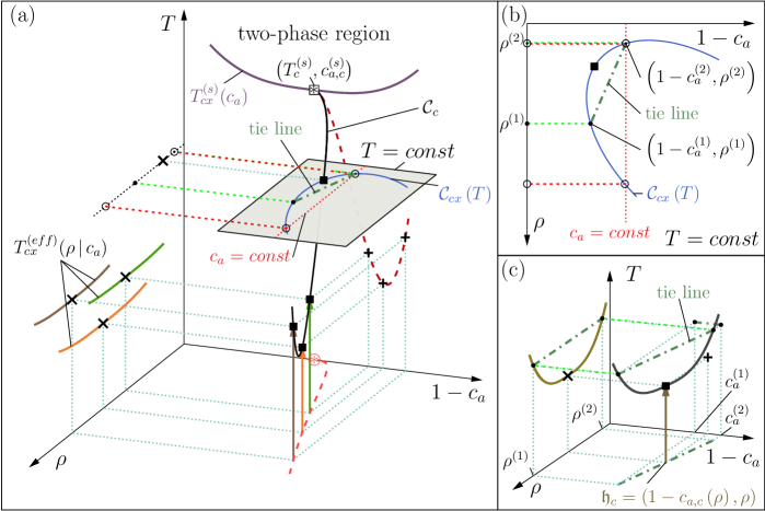
Figure 1: Sketch of the phase diagram for colloids immersed in a binary liquid mixture, the latter exhibiting a closed-loop miscibility gap. We focus on the region around the lower critical point $\boxast$ ($T^{\left(s\right)}_{c},c_{a,c}^{(s)},\rho=0$) (see the lavender phase separation curve $T^{\left(s\right)}_{cx}\!\left(c_{a}\right)$ in the $\left(T,c_{a},\rho=0\right)$ plane). For fixed pressure corresponding to a liquid state of the system, the thermodynamic (td) space of the pure solvent is two-dimensional; here we consider as variables the temperature $T$ and the concentration $c_{a}$. Upon adding colloids at fixed pressure the td space becomes three-dimensional; we use the colloidal number density $\rho$ as additional td variable. The miscibility gap of the pure solvent in the $\left(T,c_{a},\rho=0\right)$-plane extends to a two-phase region in the three-dimensional td space and is bounded by a two-dimensional manifold $T_{cx}\left(c_{a},\rho\right)$ of coexisting states (not shown). The tube-like shape of $T_{cx}\left(c_{a},\rho\right)$ is not straight but bent and twisted. Its actual form is expected to depend sensitively on all interactions (i.e., the solvent-solvent, the solvent-colloid, and the colloid-colloid interactions). Each state on $T_{cx}\left(c_{a},\rho\right)$ coexists with another one, both being connected by a horizontal and straight, so-called tie line (green dash-dotted line). There is a line $\mathcal{C}_{c}$ (black curve) of critical points (some of which are shown as black squares) embedded in $T_{cx}\left(c_{a},\rho\right)$ which is the extension of the critical point $\left(T^{\left(s\right)}_{c},c_{a,c}^{(s)},\rho=0\right)$. $\mathcal{C}_{c}$ is given by the states for which the tie line has zero length. The projections of $\mathcal{C}_{c}$ (with selected critical points ▮) onto the planes $\left(\rho,c_{a}\right)$ and $\left(T,c_{a}\right)$ (with $\boldsymbol{\mathrm{+}}$ as the projection of ▮) are indicated as red dashed curves. For $\rho\to 0$ the bending of the curve $\mathcal{C}_{c}$ can be inferred from scaling arguments (Eq. (29)). For colloidal suspensions interacting via an effective potential which consists of a soft repulsion and the critical Casimir attraction, the results of the effective approach suggest that, for intermediate values of $\rho$, $\mathcal{C}_{c}$ bends up again (see Subsect. III.2.4). This bending is due to the specific properties of the critical Casimir forces and is indicated in (a). Effective colloidal models render coexistence curves $T^{{(eff)}}_{cx}\!\left(\rho\,|\,c_{a}\right)$ which are explicit functions of $\rho$ only and depend parametrically on the overall concentration $c_{a}$ (see (a) for three examples; the three vertical arrows indicate thermodynamic paths describing the approach of the corresponding critical point ▮ upon raising temperature). For suitable effective models and within a certain region of the td space (see main text), the critical points ($\boldsymbol{\times}$), $\left(T^{{(eff)}}_{c}\left(c_{a}\right),\rho_{c}\left(c_{a}\right)\right)$, of the coexistence curves $T^{{(eff)}}_{cx}\!\left(\rho\,|\,c_{a}\right)$ are expected to approximate the projection of $\mathcal{C}_{c}$ onto the $\left(T,\rho\right)$-plane. Within the effective approach a unique value $c_{a}$ is taken throughout the whole system. In contrast, all three panels show that in general for $T=const$ the coexisting phases (i.e., the points connected by a tie-line) differ both in $\rho$ and $c_{a}$. Thus the effective approach has a limited applicability for determining the phase diagram. Experimentally, upon increasing temperature one is able to determine a (in general nonplanar) coexistence curve (black line in (c)) in the three-dimensional td space. In (c), for a selected critical value $\mathfrak{h}_{c}=\left(1-c_{a,c}\left(\rho\right),\rho\right)$ (i.e., $\mathfrak{h}_{c}$ is a point on the red dashed line in the $\left(\rho,c_{a}\right)$-plane) such a curve (black line), its projection onto the $\left(T,\rho\right)$-plane (mustard line), as well as a selected tie line and its three projections are shown. Note that the tie line is not parallel to the $\rho$-axis. This means that the coexisting phases differ with respect to $c_{a}$, in contrast to the aforementioned assumption of an unique value of $c_{a}$ for the effective one-component description. Thus the mustard curve in (c) will in general differ from the corresponding curve $T^{{(eff)}}_{cx}\!\left(\rho\,|\,c_{a}\right)$ in (a), even if the associated critical points are the same.

In this section, we consider pair potentials which are repulsive at short distances (i.e., $a$ is sufficiently large) so that the suspension is stable.

III.2.1 General discussion

In this Subsection we consider the thermodynamics of actually ternary colloidal suspensions with binary solvents such as water-lutidine mixtures which exhibit a closed-loop two-phase region of demixed phases (each being rich in one of the two species). We focus on that region of this miscibility gap which is close to the lower critical point. For fixed pressure, their thermodynamic states can be characterized by the temperature $T$ and the concentration $c_{a}$ of one of the species with the critical point $\left(T^{\left(s\right)}_{c},c_{a,c}^{(s)}\right)$ and the liquid-liquid phase coexistence curve $T^{\left(s\right)}_{cx}\!\left(c_{a}\right)$ in the absence of colloids. Upon adding colloidal particles to such a solvent, for fixed pressure the thermodynamic space of the system becomes three-dimensional spanned by $T$, $c_{a}$, and, e.g., by the colloidal number density $\rho$ (see Fig. 1; one can also choose, instead, the fugacity of the colloids). Accordingly, the closed-loop phase coexistence curve $T^{\left(s\right)}_{cx}\!\left(c_{a}\right)$ becomes a two-dimensional, tubelike manifold $T_{cx}\left(c_{a},\rho\right)$ with $T_{cx}\left(c_{a},\rho=0\right)=T^{\left(s\right)}_{cx}\!\left(c_{a}\right)$. It contains a line $\mathcal{C}_{c}$ of critical points $\left(T_{c}\left(\rho\right),c_{a,c}\left(\rho\right)\right)$ which is the extension of the critical point of the solvent in the absence of colloids, i.e., $\left(T_{c}\left(\rho=0\right),c_{a,c}\left(\rho=0\right)\right)=\left(T^{\left(s\right)}_{c},c_{a,c}^{(s)}\right)$. For fixed temperature $T=const$, the set of pairs $\left[\left(c_{a}^{\left(1\right)},\rho^{\left(1\right)}\right),\left(c_{a}^{\left(2\right)},\rho^{\left(2\right)}\right)\right]$ of coexisting states given by $T=T_{cx}\!\left(c_{a},\rho\right)$ forms a curve $\mathcal{C}_{cx}\left(T\right)$ in the $\left(c_{a},\rho\right)$ plane, the shape of which depends on the considered value of $T$ (see Figs. 1(a) and (b)). In the phase diagram, two coexisting states are connected by a straight, so-called tie line (see Fig. 1). (If one chooses the fugacity of the colloids instead of $\rho$, one also obtains a tubelike manifold $T_{cx}$ of phase coexistence. However, in this case the horizontal tie lines lie in the plane of constant fugacity, i.e., parallel to the $\left(T,c_{a}\right)$-plane, because the coexisting phases share a common fugacity of the colloids.)

As stated above, the two-phase loop of the pure solvent (i.e., for $\rho=0$, bounded by $T^{\left(s\right)}_{cx}\!\left(c_{a}\right)$) extends into the three-dimensional thermodynamic space of the actual colloidal suspension ($\rho\neq 0$). Due to the presence of additional interactions and degrees of freedom one expects that the shape of this two-phase region (bounded by $T_{cx}\!\left(c_{a},\rho\right)$) is not a straight but a distorted tube. The actual shape of $T_{cx}\left(c_{a},\rho\right)$ is expected to depend sensitively on all interactions present in the ternary mixture, i.e., among the colloidal particles, between the colloidal and the solvent particles, and among the solvent particles. The relevance of the solvent-solvent interaction for the effective potential and, accordingly, for the phase behavior of the effective colloidal system has been demonstrated recently by MC studies in which various kinds of model solvents have been used Gnan-et:2011 . It is reasonable to expect that this relevance transfers also to the phase behavior of the full multi-component system. Such distortions of the phase diagram relative to that of the underlying binary mixture do occur for ternary mixtures of molecular fluids. For example, in Ref. Andon-et:1952, experimental studies of molecular ternary mixtures containing various kinds of lutidines are reported. These studies show that the upper and lower critical temperature for a closed-loop phase diagram can be tuned by varying only the concentration of the third component and that the two-phase loop can even disappear upon adding a third component. Similar experimental results are reported in Ref. Prafulla-et:1992, . Such complex phase diagrams can also be generated by adding colloidal particles to the binary solvent, as can be inferred from corresponding experimental studies Kline-et:1994 ; Jayalakshmi-et:1997 ; Koehler-et:1997 . In contrast to the molecular ternary mixtures, for the latter kind of ternary mixtures a decrease of the lower critical temperature upon adding colloids as a third component is reported.

Theoretical studies of bona fide ternary mixtures have so far been concerned with, e.g., lattice gas models terMixTheory and (additive or non-additive) mixtures of hard spheres, needles, and polymers Schmidt-et:2002 ; Schmidt:2011 . In these studies the constituents are of comparable size, i.e., their size ratios are less than ten. The peculiarity of the kind of mixtures considered here lies in the fact that the sizes of their constituents differ by a few orders of magnitude. This property distinguishes them significantly from mixtures of molecular fluids. In contrast to molecular ternary mixtures, in colloidal suspensions the colloidal particles influence the other two components not only by direct interactions but also via strong entropic effects. This is the case because their surfaces act as confinements to fluctuations of the concentration of the solvent and they also generate an excluded volume for the solvent particles. The importance of considering the colloidal suspension as a truely ternary mixture has been already pointed out in Ref. Sluckin:1990, .

III.2.2 Scaling of the critical point shift

For dilute suspensions, i.e., for $\rho\to 0$, the shape of the line $\mathcal{C}_{c}$ of the critical points can be estimated by resorting to phenomenological scaling arguments similar to the ones given by Fisher and Nakanishi Fisher-et:1981 for a critical medium confined between two parallel plates separated by a distance $L$. For a dilute suspension, the mean distance $\rho^{-1/d}$ between colloidal particles plays a role analogous to $L$. Close to the critical point of the solvent, due to $\xi\sim\left|t\right|^{-\nu}$ one can identify the two relevant scaling variables $w^{\left(1\right)}\propto\left|t\right|^{-\Delta}h_{b}$ and $w^{\left(2\right)}\propto\left|t\right|^{\nu}\rho^{-1/d}$ (for the simplicity of the argument note_CP_scaling here we do not consider the influence of the scaling variable $\left|t\right|^{\nu}R$) and propose the scaling property ${\mathfrak{f}}\left(T,\Delta\mu,\rho\right)\simeq\left|t\right|^{2-\alpha}K\left(w^{\left(1\right)},w^{\left(2\right)}\right)$ of the free energy density (where the difference $\Delta\mu\sim h_{b}$ of the chemical potentials of the two components of the solvent acts as a symmetry breaking bulk field). The critical points are given by singularities in $K$ occurring at certain points $\left(w^{\left(1\right)}_{c},w^{\left(2\right)}_{c}\right)$. This implies that the critical point $\left(T_{c}\left(\rho\right),h_{b,c}\left(\rho\right)\right)$ shifts according to

$$T_{c}\left(\rho\right)-T^{\left(s\right)}_{c}{}\sim\rho^{1/\left(\nu d\right)}\qquad\text{and}\qquad h_{b,c}\left(\rho\right)\sim\rho^{\Delta/\left(\nu d\right)}$$ (29a)

so that

$$c_{a,c}\left(\rho\right)-c_{a,c}^{(s)}\sim\rho^{\Delta/\left(d\delta\nu\right)}$$ (29b)

with $\left(1/\left(\nu d\right)\right)_{d=3}\simeq 0.53$ and $\left(\Delta/\left(d\delta\nu\right)\right)_{d=3}\simeq 0.17$. This states that in the presence of colloids the critical point occurs when the bulk correlation lengths $\xi$ and $\xi^{\left(h\right)}$ of the solvent become comparable with the mean distance $\rho^{-1/d}$ between the colloids.

III.2.3 Effective one-component approach

Integrating out the degrees of freedom associated with the smallest components of the solution (here two) provides a manageable effective description of colloidal suspensions. This kind of approach is commonly used, for instance, recently for studying large particles immersed in various kinds of model solvents Gnan-et:2011 or in order to describe a binary mixture of colloids immersed in a phase separating solvent Zvyagolskaya-et:2011 . However, this effective description has only a limited range of applicability for investigating the phase behavior of colloidal suspensions. For example, it fails in cases in which the influence of a set of colloids on the solvent cannot be neglected or the (pure) solvent undergoes a phase seperation on its own, as considered here. In the effective approach, the concentration $c_{a}$ of one of the solvent species, averaged over the whole sample, enters as a unique parameter into the effective interaction potential between the large particles (see the dependence on $\Sigma$ in Eqs. (22) and (26)). However, generically (e.g., due to the adsorption preferences of the colloids) the concentrations $c_{a}^{\left(i\right)}$ are different in the two coexisting phases $i=1,2$ (see Fig. 1) and thus, for a proper description, one would have to allow this parameter, and hence the effective potential, to vary in space. Experiments have revealed gallagher:92 ; grull:97 ; note_col_in_solvent that for suspensions very dilute in colloids with a phase separated solvent, basically all colloidal particles are populating the phase rich in the component preferred by the colloids (with concentration $c_{a}^{\left(1\right)}$). In this case the actual effective attractive interaction among the particles will be weaker than implied by the effective potential in which only the overall concentration $c_{a}<c_{a}^{\left(1\right)}$ enters as a parameter. (We recall that the CCFs depend non-monotonously on $c_{a}$ and are strongest for $c_{a}\lesssim c_{a,c}^{(s)}$. Thus for $c_{a}^{\left(2\right)}<c_{a}<c_{a}^{\left(1\right)}$ the CCFs differ for each concentration and are - for the typical situation considered here - in general weakest for $c_{a}^{\left(1\right)}$; $c_{a}^{\left(2\right)}$ is the concentration in the other coexisting phase.) Within the effective approach for the colloids, one obtains, e.g., by means of DFT, coexistence curves $T^{{(eff)}}_{cx}\!\left(\rho\,|\,c_{a}\right)$ which depend parametrically on the solvent composition $c_{a}\approx c_{a,c}^{(s)}$ (or equivalently, by making use of Eq. (33), on $\Sigma$ as in Eq. (26)). Since the effective potential corresponding to this specific value of $c_{a}$ is used both for the one-phase region as well as for both phases within the two-phase region, this implies that the tacitly assumed corresponding physical situation is such that the composition $c_{a}$ is fixed throughout the system as an external constraint. In particular the two coexisting phases do not differ in their values of the concentration of the solvent particles but only in their colloidal densities $\rho^{\left(1\right)}$ and $\rho^{\left(2\right)}$. Thus within the effective approach for determining the phase behavior one of the essential features, i.e., the tendency of the solvent to phase separate, is suppressed. Accordingly, it is not possible to construct the full coexistence manifold $T_{cx}\!\left(c_{a},\rho\right)$ on the basis of the curves $T^{{(eff)}}_{cx}\!\left(\rho\,|\,c_{a}\right)$ alone. Rather, the effective approach is adequate as long as to a large extent the phase segregation involves only the colloidal degree of freedom, i.e., the values of $\rho$ differ in the two phases, but the values of $c_{a}$ are nearly the same. Therefore the approximation $T_{cx}\left(c_{a},\rho\right)\approx T^{{(eff)}}_{cx}\!\left(\rho\,|\,c_{a}\right)$ is valid in a region of the thermodynamic space in which the actual tie lines happen to be almost orthogonal to the $c_{a}$-axis (see Fig. 1). For the phase diagram in terms of the variables $T$, $c_{a}$, and the fugacity of the colloids this latter condition implies that the tie lines have to be sufficiently short.

We expect the effective one-component approach to work well for temperatures corresponding to the one-phase region of the pure solvent and for an intermediate range of values of $\rho$. On one hand $\rho$ should be large enough so that the competition between the configurational entropy and the potential energy due to the effective forces can drive a phase separation. On the other hand $\rho$ has to be small enough so that the approximation of using an effective pair potential between the colloids is valid and the influence of the colloids on the phase behavior of the solvent is subdominant. Given such values of $\rho$ and $T$, the reduced second virial coefficient $B_{2}^{*}$ (Eq. (14)) is an appropriate measure for the strength of the attraction and a useful indicator of the occurrence of a phase separation into a colloidal-rich (“liquid”) and a colloidal-poor (“gas”) phase. According to the discussion above, for values of the thermodynamic variables (i.e., the values of $T$ and $\rho$, and for the prescribed value of $c_{a}$) which are approximately the same as in the one-component approach, the ternary mixture is expected to exhibit a phase separation. According to the VLNF conjecture the corresponding critical point should occur when $B_{2}^{*}$ reaches the critical value $B_{2,c}^{*}\simeq-1.212$ (Eq. (14)) of Baxter’s model. While the VLNF conjecture provides an empirical estimate for the values of parameters for which there is a critical point, within DFT these parameters as well as the shape of the phase coexistence curve can be calculated. Within the effective approach only its dependence on the colloidal density number $\rho$ for globally fixed values of $c_{a}$ can be determined.

III.2.4 Phase diagrams

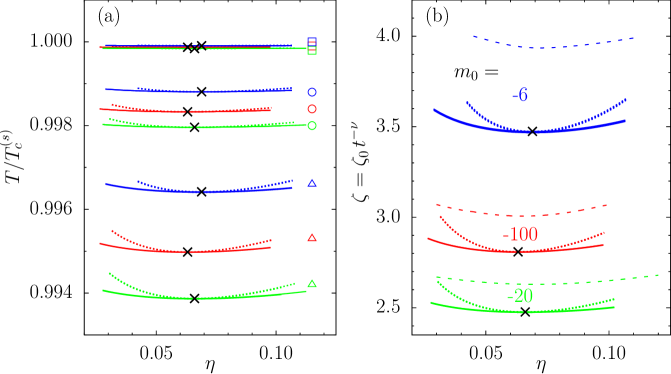
Figure 2: (a) Phase coexistence curves $T^{{(eff)}}_{cx}(\rho\,|\,c_{a})$ (full lines), spinodals (mean-field divergence of $\chi_{T}$, dotted lines), and the critical points $T^{(eff)}_{c}$ (crosses) of an effective, one-component system of large particles (Eq. (26)) as obtained by DFT according to Eq. (18). The curves correspond to a solvent with a lower critical temperature $T^{\left(s\right)}_{c}$ and to various fixed solvent compositions $c_{a}$ ($m_{0}=-100$ (red), $-20$ (green), $-6$ (blue)). The other parameters are taken as $\zeta_{0}=0.01\;\left(\Box{}\right)$, $0.05\;\left(\circ\right)$, and $0.1\;\left(\vartriangle\right)$, $s=10$, and $aT/T^{\left(s\right)}_{c}=100$. Close to the phase separation, the dominant temperature dependence is that of the critical Casimir forces (CCFs) encoded in $\zeta\left(t=1-T/T^{\left(s\right)}_{c}\right)=\mathop{sgn}\left(t\right)\kappa\xi\left(t\right)=\mathop{sgn}\left(t\right)\zeta_{0}\left|t\right|^{-\nu}$. Therefore, in terms of $\zeta$ (see panel (b)) the curves in (a) for different values of $\zeta_{0}$ fall de facto on top of each other, independent of whether the solvent has an upper or a lower critical point. Within the integral equation approach only the spinodals have been determined (PY: dashed lines in (b), see the main text). According to Eq. (27), $\left(c_{a}-c_{a,c}^{(s)}\right)^{-1}\sim m_{0}=\pm\infty$ corresponds to the critical composition $c_{a,c}^{(s)}$. For solvent compositions which are somewhat poor in the component preferred by the colloids, i.e., for intermediate negative values of $m_{0}\simeq-20$, the CCFs are strongly attractive. Therefore, for them small correlation lengths suffice to bring about phase separation; accordingly the binodals occur at small values of $\zeta\sim\left|t\right|^{-\nu}$. Here we consider only thermodynamic states of the solvent which are in the one-phase region, i.e., $t>0$.

Generically, in experiments the solvent composition and hence the associated quantity $m_{0}$ (Eq. (27)) is fixed and $\zeta\sim\left|t\right|^{-\nu}$ is varied. In Fig. 2(a) for a solvent exhibiting a lower critical point and for the parameter choices $aT/T^{\left(s\right)}_{c}=100$, $s=10$, $m_{0}=-100$, $-20$, and $-6$, and $\zeta_{0}=0.01$, $0.05$, and $0.1$ we present the coexistence curves $T^{{(eff)}}_{cx}(\rho\,|\,c_{a})$ and the spinodals of the colloidal “liquid”-“gas” phase transition as function of the colloid packing fraction $\eta=(4\pi/3)R^{3}\rho$ as obtained by the DFT presented in Eq. (18). (Note that in accordance with Eqs. (2) and (26) in the product $aT$ the explicit dependence on $T$ drops out.) For the corresponding free energy $\mathcal{F}_{RPA}$ given in Eq. (19) the effective colloidal system phase separates if $\widetilde{U}_{a,0}<\left(\widetilde{U}_{a,0}\right)_{c}=-21.3$. This condition is satisfied provided the attractive part of the interaction potential is sufficiently strong. We recall, that for the effective potential considered here attraction occurs for $T/T^{\left(s\right)}_{c}=1\pm\left(\zeta/\zeta_{0}\right)^{-1/\nu}\to 1$ (see Eq. (26)). For a solvent exhibiting a lower (upper) critical point the lower (upper) sign holds in the one-phase region of the solvent, within which the effective approach is applicable. In this temperature limit the variation of $a$ (Eqs. (2) and (26)) with $T$ is subdominant and thus the dependence of $\mathcal{F}_{RPA}$ on $T/T^{\left(s\right)}_{c}$ and $\zeta_{0}$ reduces to a dependence on $\zeta$ only. Accordingly, as can be inferred from the comparison of Figs. 2(a) and 2(b), in terms of $\zeta$ for each value of $m_{0}$ the coexistence curves $T^{{(eff)}}_{cx}(\rho\,|\,c_{a})$ for different values of $\zeta_{0}$ fall de facto on top of each other. The difference between these curves is of the order of $\left(\zeta_{0}/\zeta\right)^{1/\nu}$ (because $T/T^{\left(s\right)}_{c}=1\pm\left(\zeta/\zeta_{0}\right)^{-1/\nu}$), which for the three values of $\zeta_{0}$ used in Fig. 2 is about the thickness of the lines shown in Fig. 2(b). In terms of this presentation it does not matter whether the solvent exhibits a lower or an upper critical point. Although spinodals are mean-field artifacts, we present them nonetheless because they provide some indication about the location of the binodal which encloses the former. Furthermore the spinodals carry the advantage that the isothermal compressibility $\chi_{T}$ is the property of only one thermodynamic state. Therefore, in contrast to the calculation of the binodal (which depends on two coexisting phases), the calculation of the spinodal does not suffer from the non-uniqueness of the effective potential in the case of phase coexistence. As discussed in Subsect. II.1.2, based on formally exact relations the phase behavior can in principle be calculated from the correlation functions obtained within the integral equation approach (IEA). Within the so-called compressibility route (Eq. (5)) the spinodals, i.e., the loci of the mean-field divergence of $\chi_{T}$, are directly accessible. On the other hand, the binodals, i.e., the loci of two thermodynamic states which at the same temperature have different packing fractions but the same pressure, are directly accessible via the so-called virial route (Eq. (4)). We refrain from calculating the binodal (the spinodal) via the compressibility route (virial route), because it would require thermodynamic integration, which we want to avoid due to the subtlenesses described in Subsect. II.1.2. The spinodals calculated by the compressibility route are shown as dashed curves in Fig. 2(b). For the region of the thermodynamic space where the IEA renders solutions for the correlation functions, we failed to find binodals, i.e., along the pressure isotherms $p\left(\eta;T=const\right)$ as calculated via the virial route there are no two states with $\eta_{1}\neq\eta_{2}$ and $p\left(\eta_{1};T\right)=p\left(\eta_{2};T\right)$. These observations can be explained by the thermodynamic inconsistency of this IEA. Due to the approximate bridge function, the binodals as obtained by two different routes need not to coincide. The same observations are found within the HNC approximation within which the spinodals are shifted w.r.t. to the PY results to slightly smaller values of $\zeta$. Although within the IEA the binodals could not be determined, at least the loci of the obtained spinodals are similar to the ones obtained from DFT.

Since the CCFs are strongest for slightly off-critical compositions $m_{0}^{-1}\sim\left(c_{a}-c_{a,c}^{(s)}\right)\lesssim 0$ the binodals (and spinodals) are shifted to smaller values of $\zeta$ upon decreasing $\left|m_{0}\right|$ down to $m_{0}\simeq-20$. With a further decrease of $\left|m_{0}\right|$ the system moves too far away from the critical point of the solvent so that the CCF weakens and the spinodals shift again to larger values of $\zeta$.

The critical value $\eta_{c}$ of the packing fraction is rather small, i.e., $\eta_{c}\approx 0.07$ (see Fig. 2), because the effective hard sphere diameter $\sigma$ which results from the soft repulsion $U_{rep}$ is larger than $2R$. In terms of $\eta_{\sigma}=(\sigma/(2R))^{3}\eta$ (defined after Eq. (19)) the critical value assumes its RPA-value $\eta_{\sigma,c}^{\left(RPA\right)}=0.129$. Furthermore, the binodals shown in Fig. 2 are rather flat compared with, e.g., the ones for hard spheres interacting via a short-ranged, attractive temperature independent potential (described also by Eq. (19)). In the present system, the deviation from the critical temperature $T_{c}$ which leads to a range of $\eta$ for the coexisting phases as large as shown in Fig. 2, is about $1$‰, whereas for a system of hard spheres with an attraction the corresponding temperature deviation is a few percent. For smaller values of $\zeta_{0}$ the binodals are flatter and the differences of the critical temperatures for different values of $m_{0}$ are smaller (see Fig. 2(a)). The requirement $\eta^{-1/3}>\left(4\pi/3\right)^{1/3}\left(2+\zeta/s\right)$ (see Subsect. II.2.2) concerning the validity of the pairwise approximation for the CCFs is fulfilled for the whole range of values for $\eta$ and $\zeta$ shown in Fig. 2; e.g., for $s=10$ and $\zeta=4$ the above condition is $\eta<0.3$.

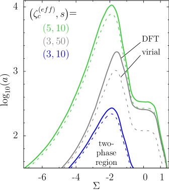
Figure 3: Attraction due to CCFs can induce a “liquid”-“gas” phase separation of the colloids. Within the effective approach described by Eq. (26) the dominant temperature dependence is that of the Casimir scaling function encoded in $\zeta=\kappa\xi\left(t\right)\sim\left|t\right|^{-\nu}$. The full curves correspond to DFT (Eq. (18)) and show for which values of $\Sigma$ and $a$ corresponding to the solvent composition and the repulsive strength of the background potential, respectively, a given temperature (in terms of $\zeta$) is the critical one $T^{(eff)}_{c}$ or $\zeta^{(eff)}_{c}$. The contour lines $a\left(\Sigma;s;\zeta_{c}^{\left(eff\right)}\right)$ depend parametrically on $s=\kappa R$ where $\kappa^{-1}$ is the range of the background repulsion and $R$ is the radius of the colloids. Systems, with their parameters being located in the area below the contour line $\zeta^{(eff)}_{c}$, are phase separated at this temperature. This two-phase region expands to larger values of $a$ with increasing $\zeta$. For a fixed value $\zeta^{(eff)}_{c}$, $a\left(\Sigma;s;\zeta_{c}^{\left(eff\right)}\right)$ is largest for compositions slightly poor in the component preferred by colloids, i.e., $\Sigma\lesssim 0$. In addition, the corresponding contour lines based on the VLNF criterion $B_{2}^{*}\left(\zeta=\tilde{\zeta}^{(eff)}_{c},\Sigma,a;s\right)=B_{2,c}^{*}$ for the reduced second virial coefficient (Eq. (14)) are plotted as dashed lines. It is satisfactory to see that both approaches provide comparable results.

The sketch of the phase diagram in Fig. 1 and the calculated coexistence curves in Fig. 2 correspond to using the background potential with fixed parameters $s$ and $a$. In order to investigate the dependence of the locus of the phase separation on properties of the background potential, in the following we shall discuss how the critical temperature $T^{(eff)}_{c}=T^{(eff)}_{c}\left(\Sigma,a,s,\zeta_{0},T^{\left(s\right)}_{c},\pm\right)$ of the effective colloidal system varies as function of its arguments ($\pm$ is taken to be $-$ and $+$ for a lower and an upper critical point, respectively). According to the discussion above, to this end it is sufficient to determine $\zeta^{(eff)}_{c}\left(\Sigma,a,s\right)$. In Fig. 3 for fixed values of $s$ and for specific values of $\zeta^{(eff)}_{c}$ we show the contour lines $a=a\left(\Sigma;s;\zeta^{(eff)}_{c}\right)$. That is, for a colloidal system with a background potential characterized by certain values of $a$ and $s$, from the plot in Fig. 3 one can read off the value of the difference of the chemical potentials of the two components of the solvent (which is related to $\Sigma$) for which $T^{(eff)}_{c}$ has a prescribed value. The full curves are calculated within the density functional approach (Eq. (18)) and are compared with the ones corresponding to the simple prediction (Eqs. (13) and (26)) $B_{2}^{*}\left(\zeta=\tilde{\zeta}^{(eff)}_{c},\Sigma,a;s\right)=B_{2,c}^{*}=-1.212$, which also yields a relation $\tilde{\zeta}^{(eff)}_{c}=\tilde{\zeta}^{(eff)}_{c}\left(\Sigma,a;s\right)$. Both approaches differ only slightly. For given values of $\zeta_{c}^{\left(eff\right)}$ and $\Sigma$ the VLNF conjecture predicts a smaller critical value of $a$ than obtained from DFT. The largest deviations occur for slightly negative values of $\Sigma$, for which the CCFs are more attractive. For all values of the parameters shown in Fig. 3 (i.e., $a\gtrsim 30$), at small distances $D$ the corresponding potentials exhibit repulsive barriers $\gtrsim 30k_{B}T$. For smaller values of $a$, i.e., $a\lesssim 15$, this potential barrier disappears and the colloidal particles may form aggregates. This is discussed in the following paper MMD_part2 ; see Figs. 1 and 2 therein.

The contour lines $a=a\left(\Sigma;s;\zeta^{(eff)}_{c}\right)$ attain their largest values for slightly negative values of $\Sigma$, i.e., for $\Sigma\simeq-2$. This again reflects the asymmetry of the strength of the CCFs with respect to the bulk ordering field $h_{b}$ in the presence of symmetry breaking surface fields. In Fig. 3, for all parameter pairs $\left(a,\Sigma\right)$ below each contour line, characterized by $\zeta^{(eff)}_{c}$, the corresponding system at the temperature belonging to the value $\zeta^{(eff)}_{c}$ is phase separated. This two-phase region widens with increasing values of $\zeta$ and it significantly expands to larger values of $a$, which is in line with the fact that the CCFs become stronger upon approaching $T^{\left(s\right)}_{c}$. For $s=10$, upon increasing $\zeta^{(eff)}_{c}$ from $3$ to $5$ the largest critical value of $a$ increases by two orders of magnitude (compare the corresponding blue and green curves in Fig. 3). The two-phase region can be markedly increased upon increasing $s$ (compare the blue and gray curves in Fig. 3 corresponding to $\zeta_{c}^{\left(eff\right)}=3$ with $s=10$ and $s=50$, respectively) because for the phase separation the strength of the attraction is important; due to $U\sim s$ (Eq. (26)) the latter can be easily tuned by varying $s$.

For the experimental studies reported in Refs. Kline-et:1994, ; Jayalakshmi-et:1997, colloidal mixtures consisting of silica spheres, water, and 2-butoxyethanol or lutidine have been used; with a radius $R\approx 11nm$ the colloidal particles have been rather small. Thus, a priori, the effective approach, developed in Subsect. II.1 and discussed in Subsect. III.2.3, is not expected to apply. Nonetheless, one can try to do so and estimate the critical temperature for solutions containing such small particles by using the general scaling arguments presented in Subsect. III.2.2 and in Ref. note_CP_scaling, . At the critical temperature, the dimensionless scaling variable $w^{(3)}=w_{0}^{(3)}\left|t\right|^{\nu}R$ associated with the radius of the colloid takes on a certain value $w_{c}^{(3)}$ with $w_{c}^{(3)}/w_{0}^{(3)}=\left|\left(T^{\left(s\right)}_{c}-T_{c}(\rho)\right)/T^{\left(s\right)}_{c}\right|^{\nu}R\equiv\left|t_{c}\right|^{\nu}R$ (where $w_{0}^{(3)}$ is a non-universal amplitude). Using our effective approach we can calculate $w_{c}^{(3)}/w_{0}^{(3)}$ within mean-field theory for parameters corresponding to the solvents used in those experiments, and demand note_w3c that this ratio applies approximately to the experiments reported in Refs. Kline-et:1994, ; Jayalakshmi-et:1997, . For the solvents used, the relevant parameters are $\xi_{0}\approx 0.25nm$ and $\zeta_{0}\sim 0.03$. Choosing $s=10$ (see Subsect. III.1 and Fig. 2(a)) renders $R=\xi_{0}s/\zeta_{0}\approx 85nm$. This value of $R$ is sufficiently large so that the aforementioned effective approach can be considered to be reliable. From Fig. 2(a) we can read off the corresponding shift $\left|t_{c}\right|\sim 0.001$ which leads to $w_{c}^{(3)}/w_{0}^{(3)}\simeq 1.094nm$. By using this latter mean-field estimate, for the experimental value $R\approx 11nm$ of the radius of the colloidal particles one thus obtains the shift $\left|t_{c}\right|=\left(w_{0}^{(3)}R/w_{c}^{(3)}\right)^{-1/\nu}\simeq 0.234$. With the critical temperature $T^{\left(s\right)}_{c}\approx 320K$ of the solvent Kline-et:1994 ; Jayalakshmi-et:1997 , this leads to $T_{c}\left(\rho\right)=\left(1-t_{c}\right)T^{\left(s\right)}_{c}\approx 310K$. Indeed, for such a temperature phase separation in the ternary mixture has been observed (although even lower critical temperatures $T_{c}\approx 300K$ have been reported Kline-et:1994 ; Jayalakshmi-et:1997 ). As stated above such an agreement for even small colloids could not have been anticipated from the outset.

IV Summary

We have studied the collective behavior of monodisperse colloidal suspensions with near-critical solvents. Colloidal particles acting as cavities set the boundary conditions for the fluctuating order parameter (OP) of the solvent and perturb the OP field on the length scale of the bulk correlation length $\xi\left(t=\left(T-T^{\left(s\right)}_{c}\right)/T^{\left(s\right)}_{c}\to 0\right)\sim\left|t\right|^{-\nu}$, which diverges upon approaching the critical temperature $T^{\left(s\right)}_{c}$; $\nu$ is a critical bulk exponent. These modifications of the OP and restrictions of its fluctuation spectrum result in an effective force acting between the colloids, known as the critical Casimir force (CCF). For equal boundary conditions (BCs), i.e., equal surface properties of all colloids, the CCF is attractive. The CCF depends on the configuration of all colloidal particles and thus is in general non-additive. We have obtained our results for an effective one-component system of colloids interacting via an effective pair potential. The regular background potential has been taken to be a soft repulsion acting on a length scale $\kappa^{-1}$ and with strength $A$. We have considered suspensions with medium values of the colloidal number density $\rho$, for which the approximation of pairwise additive CCFs is valid. The scaling function of the critical Casimir potential has been taken in accordance with the Derjaguin approximation (Eq. (23)), within which the pair potential between two spheres is expressed in terms of the scaling function of the CCF in a slab. The variation of the scaling function in a slab with the scaling variable $\Sigma$ associated with the bulk ordering field $h_{b}$ (see Eq. (3)) in spatial dimension $d=3$ has been approximated based on Monte Carlo simulation data and on mean-field theory results (Eq. (24)). On this basis we have obtained the following main results:

1. In Fig. 1 we have illustrated the phase behavior of a ternary mixture consisting of colloidal particles and a binary solvent which exhibits a miscibility gap. We have discussed in detail the relationship between this full description and the one which is based on an effective, one-component colloidal fluid (Fig. 1).

2. For certain regions of the three-dimensional thermodynamic space $\left(T,c_{a},\rho\right)$ of a ternary mixture, the effective one-component model is applicable for obtaining the onset of phase separation. For particles interacting via the effective pair potential given in Eq. (26) we have calculated the phase coexistence curve and the spinodal (i.e., the loci where within mean-field theory the isothermal compressibility $\chi_{T}$ diverges) both within density functional theory (DFT, Eq. (18)) and the integral equation approach. In Fig. 2 the coexistence curves for various values of $c_{a}-c_{a,c}^{(s)}\sim m_{0}^{-1}$ are shown. The spinodals as obtained by using the DFT approach are narrower and are located at smaller values of $\zeta=\kappa\xi\sim\left|t\right|^{-\nu}$ than the ones obtained from the integral equation approach.

3. In Fig. 3 the dependence of the critical temperature of the effective one-component system (expressed in terms of $\zeta^{(eff)}_{c}$) on the parameters $a=A/s$, $\Sigma$, and $s=\kappa R$ is shown. For a given value of $a$, $\zeta^{(eff)}_{c}$ is smallest for slightly negative values of $\Sigma$. The critical temperature has been calculated within DFT and compared with the simple prediction $B_{2}^{*}=B_{2,c}^{*}$ as suggested by Vliegenthart and Lekkerkerker Vliegenthart-et:2000 and Noro and Frenkel Noro-et:2000 ; $B_{2}^{*}$ is the reduced second virial coefficient (Eqs. (13) and (14)) and $B_{2,c}^{*}$ is the critical value of Baxter’s model. Both approaches yield good agreement.

To conclude, our results show that the CCF, which can be easily controlled by temperature $T$ and the strength and range of which can be varied by changing the bulk ordering field $h_{b}$, can induce phase separation into a colloidal-poor and a colloidal-rich phase. Within the approach of using an effective potential, we have identified the ranges of values for the background repulsive potential and the values of the scaling variables associated with the critical solvent, for which the colloids phase separate. We have used the approach developed here in order to study also the stability of colloidal suspensions in near-critical binary solvents MMD_part2 .

Concerning further research, more complex suspensions could be considered, for example a mixture of colloids with different adsorption preferences for the solvent particles. According to Gibbs’ phase rule, for such a four-component system (a binary mixture of colloids in a binary solvent) at constant pressure a two-dimensional manifold of critical points embedded in a three-dimensional manifold of coexisting states in the (then four-dimensional) thermodynamic space can be expected. Recently, such a mixture was studied experimentally Zvyagolskaya-et:2011 . In this study, concerning the effective interaction potential of the CCFs between the colloids the attractive $\left(+,+\right)$ BCs and the repulsive $\left(+,-\right)$ BCs were realized for colloidal particles of the same kind and for particles of different kind, respectively. In line with an effective DFT, upon approaching the critical temperature of the solvent there are indications that these two kinds of particles phase separate.

In order to study the phase behavior of the actual three- or four-component mixture for the full range of all thermodynamic variables $T$, $c_{a}$, and $\rho$, an analysis beyond the effective approach is needed.

Appendix A Off-critical mixtures

The Hamiltonian given in Eq. (20) depends on the reduced temperature $t$ and the bulk field $h_{b}$, which for a binary liquid mixture is proportional to the deviation of the difference of the chemical potentials of the two components $a$ and $b$ from its critical value, i.e., $h_{b}\sim\left(\mu_{a}-\mu_{b}\right)-\left(\mu_{a,c}-\mu_{b,c}\right)$ for a fixed pressure $\sim\mu_{a}+\mu_{b}$. Accordingly, for fixed $h_{b}$ the OP varies upon changing $t$. However, in most experimental realizations $t$ is varied at fixed concentrations $c_{i}$, $i\in\left\{a,b\right\}$, and thus the OP is kept constant. The OP $\phi$, which is not uniquely defined, is related to the ordering field $h_{b}$ by the equation of state (EOS) which for a critical system takes the scaling form Pelissetto-et:2002

$$h_{b}=\mathcal{D}\mathop{sgn}(\phi)\left|\phi\right|^{\delta}F\left(t\left|\mathcal{B}/\phi\right|^{1/\beta}\right),$$ (30)

or equivalently

$$\phi=\mathop{sgn}\left(h_{b}\right)\mathcal{B}\left|t\right|^{\beta}G\left(\mathcal{B}^{1/\beta}\mathcal{D}^{1/\left(\delta\beta\right)}t\left|h_{b}\right|^{-1/\left(\delta\beta\right)}\right)$$ (31)

with universal scaling functions $F\left(\hat{X}\right)$ and $G\left(Y\right)$ with $G\left(Y\to 0\right)=\left|Y\right|^{-\beta}$. $\mathcal{D}$ and $\mathcal{B}$ are non-universal amplitudes which depend on the definition of $\phi$ such that on the coexistence curve the bulk OP follows $\phi_{b}\left(t\to 0^{-},h_{b}=0\right)=\mathcal{B}\left|t\right|^{\beta}$. $\mathcal{D}$, $\mathcal{B}$, and the correlation length amplitudes $\xi_{0}^{\pm,h}$ (defined after Eq. (21)) are related to each other by universal amplitude ratios such that only two of them are independent Pelissetto-et:2002 ; colloids1b . In the lowest order in its argument

$$\hat{X}=t\left|\mathcal{B}/\phi\right|^{1/\beta},$$ (32)

the universal scaling function $F$ has the functional form $F\left(\hat{X}\right)=1+\hat{X}$, which captures the crossover between the critical behavior at $t=0$ and at $h_{b}=0$, respectively Pelissetto-et:2002 . At the coexistence curve one has $t<0$ and $h_{b}=0$; therefore $\hat{X}=-1$ in agreement with $\phi=\mathcal{B}\left|t\right|^{\beta}$. Along the critical isotherm $t=0$ one has $\hat{X}=0$ and thus $\phi=\mathop{sgn}\left(h_{b}\right)\left|h_{b}/\mathcal{D}\right|^{1/\delta}$. For our purpose of fluid systems exposed to surfaces the sign of $\phi$ matters and the appropriate scaling variable is $X=\mathop{sgn}\left(\phi\right)\left|t\right|\left|\mathcal{B}/\phi\right|^{1/\beta}$. In terms of the scaling variables $\Sigma=\mathop{sgn}\left(h_{b}\right)\xi/\xi^{\left(h\right)}=\mathop{sgn}\left(h_{b}\right)\left(\xi_{0}^{+}/\xi_{0}^{\left(h\right)}\right){\left|h_{b}\right|^{\nu/\left(\beta\delta\right)}\left|t\right|^{-\nu}}$ and $X$, Eq. (30) takes the scaling form

$$\begin{split}\mathop{sgn}\left(\Sigma\right)\left|\Sigma\right|^{\beta\delta/\nu}&=\\ &\left(R_{\chi}\delta/Q_{2}\right)^{\delta/\left(\delta-1\right)}\left(Q_{\xi}^{+}/Q_{\xi}^{c}\right)^{\beta\delta/\nu}\\ &\times\mathop{sgn}\left(X\right)\left|X\right|^{-\beta\delta}F_{\pm}\left(\left|X\right|\right),\end{split}$$ (33)

where $F_{\pm}\left(\left|X\right|\right)=1\,\pm\,\left|X\right|$ and $\pm$ refers to the sign of $t$. $R_{\chi}$, $Q_{2}$, $Q_{\xi}^{+}$, and $Q_{\xi}^{c}$ are universal amplitude ratios Pelissetto-et:2002 . We shall use these expressions in order to calculate the variation of several experimentally accessible quantities along experimentally realizable thermodynamic paths.

References

- (1) C. N. Likos, Phys. Rep. 348, 267 (2001).
- (2) S. Asakura and F. Oosawa, J. Chem. Phys. 22, 1255 (1954); concerning systems in which adding small particles weakens the net attraction between large particles see, e.g., D. J. Ashton, J. Liu, E. Luijten, and N. B. Wilding, J. Chem. Phys. 133, 194102 (2010).
- (3) M. Dijkstra, J. M. Brader, and R. Evans, J. Phys.: Condens. Matter 11, 10079 (1999).
- (4) S. Buzzaccaro, R. Rusconi, and R. Piazza, Phys. Rev. Lett. 99, 098301 (2007).
- (5) R. Evans, J. Phys.: Condens. Matter 2, 8989 (1990).
- (6) M. E. Fisher and P. G. de Gennes, C. R. Acad. Sci., Paris, Ser. B 287, 207 (1978).
- (7) C. Hertlein, L. Helden, A. Gambassi, S. Dietrich, and C. Bechinger, Nature 451, 172 (2008).
- (8) A. Gambassi, A. Maciołek, C. Hertlein, U. Nellen, L. Helden, C. Bechinger, and S. Dietrich, Phys. Rev. E 80, 061143 (2009).
- (9) U. Nellen, L. Helden, and C. Bechinger, EPL 88, 26001 (2009).
- (10) T. W. Burkhardt and E. Eisenriegler, Phys. Rev. Lett. 74, 3189 (1995).
- (11) D. Dantchev, F. Schlesener, and S. Dietrich, Phys. Rev. E 76, 011121 (2007).
- (12) (a) M. N. Barber in Phase Transitions and Critical Phenomena, edited by C. Domb and J. L. Lebowitz (Academic, New York, 1983), Vol. 8, p. 149; (b) V. Privman, in Finite Size Scaling and Numerical Simulation of Statistical Systems, edited by V. Privman (World Scientific, Singapore, 1990), p. 1.
- (13) H. W. Diehl in Phase Transitions and Critical Phenomena, edited by C. Domb and J. L. Lebowitz (Academic, New York, 1986), Vol. 10, p. 76.
- (14) M. Krech, Casimir Effect in Critical Systems (World Scientific, Singapore, 1994); J. Phys.: Condens. Matter 11, R391 (1999).
- (15) G. Brankov, N. S. Tonchev, and D. M. Danchev, Theory of Critical Phenomena in Finite-Size Systems (World Scientific, Singapore, 2000).
- (16) More recent results for critical Casimir forces are summarized in A. Gambassi, J. Phys.: Conf. Ser. 161, 012037 (2009).
- (17) A. Hanke, F. Schlesener, E. Eisenriegler, and S. Dietrich, Phys. Rev. Lett. 81, 1885 (1998).
- (18) F. Schlesener, A. Hanke, and S. Dietrich, J. Stat. Phys. 110, 981 (2003).
- (19) S. Kondrat, L. Harnau, and S. Dietrich, J. Chem. Phys. 131, 183901 (2009).
- (20) M. Krech, Phys. Rev. E 56, 1642 (1997).
- (21) (a) Z. Borjan and P. J. Upton, Phys. Rev. Lett. 81, 4911 (1998); (b) ibid 101, 125702 (2008).
- (22) (a) M. E. Fisher and P. J. Upton, Phys. Rev. Lett. 65, 2402 (1992); (b) ibid 65, 3405 (1992).
- (23) O. Vasilyev, A. Gambassi, A. Maciołek, and S. Dietrich, EPL 80, 60009 (2007); O. Vasilyev, A. Gambassi, A. Maciołek, and S. Dietrich, Phys. Rev. E 79, 041142 (2009).
- (24) M. Hasenbusch, Phys. Rev. B 82, 104425 (2010).
- (25) M. Hasenbusch, Phys. Rev. B 83, 134425 (2011).
- (26) O. Vasilyev, A. Maciołek, and S. Dietrich, Phys. Rev. E 84, 041605 (2011).
- (27) (a) S. Buzzaccaro, J. Colombo, A. Parola, and R. Piazza, Phys. Rev. Lett. 105, 198301 (2010); (b) R. Piazza, S. Buzzaccaro, A. Parola, and J. Colombo, J. Phys.: Condens. Matter 23, 194114 (2011).
- (28) M. Fukuto, Y. F. Yano, and P. S. Pershan, Phys. Rev. Lett. 94, 135702 (2005).
- (29) S. Rafaï, D. Bonn, and J. Meunier, Physica A 386, 31 (2007).
- (30) B. Derjaguin, Kolloid Zeitschrift 69, 155 (1934).
- (31) M. Tröndle, S. Kondrat, A. Gambassi, L. Harnau, and S. Dietrich, EPL 88, 40004 (2009); M. Tröndle, S. Kondrat, A. Gambassi, L. Harnau, and S. Dietrich, J. Chem. Phys. 133, 074702 (2010); M. Tröndle, O. Zvyagolskaya, A. Gambassi, D. Vogt, L. Harnau, C. Bechinger, and S. Dietrich, Mol. Phys. 109, 1169 (2011).
- (32) S. R. Kline and E. W. Kaler, Langmuir 10, 412 (1994).
- (33) Y. Jayalakshmi and E. W. Kaler, Phys. Rev. Lett. 78, 1379 (1997).
- (34) R. D. Koehler and E. W. Kaler, Langmuir 13, 2463 (1997).
- (35) T. J. Sluckin, Phys. Rev. A 41, 960 (1990).
- (36) H. Löwen, Phys. Rev. Lett. 74, 1028 (1995).
- (37) R. R. Netz, Phys. Rev. Lett. 76, 3646 (1996).
- (38) J.-L. Barrat and J.-P. Hansen, Basic concepts for simple and complex liquids (Cambridge University Press, Cambridge, 2003).
- (39) W. B. Russel, D. A. Saville, W. R. Schowalter, Colloidal Dispersions (Cambridge University Press, 1989).
- (40) A. Pelissetto and E. Vicari, Phys. Rep. 368, 549 (2002).
- (41) J. P. Hansen and I. R. McDonald, Theory of Simple Liquids (Academic, London, 1986).
- (42) C. Caccamo, Phys. Rep. 274, 1 (1996).
- (43) K. Binder, C. Billotet and P. Mirold, Z. Physik B 30, 183 (1978).
- (44) L. S. Ornstein, and F. Zernike, Proc. Acad. Sci. Amsterdam 17, 793 (1914).
- (45) M. J. Gillan, Mol. Phys. 38, 1781 (1979).
- (46) A. J. Archer and N. B. Wilding, Phys. Rev. E 76, 031501 (2007).
- (47) (a) M. L. Kurnaz and J. V. Maher, Phys. Rev. E 51, 5916 (1995); (b) M. L. Kurnaz and J. V. Maher, Phys. Rev. E 55, 572 (1997).
- (48) G. A. Vliegenthart and H. N. W. Lekkerkerker, J. Chem. Phys. 112, 5364 (2000).
- (49) M. G. Noro and D. Frenkel, J. Chem. Phys. 113, 2941 (2000).
- (50) (a) J. Largo and N. B. Wilding, Phys. Rev. E 73, 036115 (2006); (b) G. Foffi and F. Sciortino, Phys. Rev. E 74, 050401(R) (2006); (c) P. Orea and Y. Duda, J. Chem. Phys. 128, 134508 (2008); (d) D. Gazzillo, J. Chem. Phys. 134, 124504 (2011).
- (51) R. J. Baxter, J. Chem. Phys. 49, 2770 (1968).
- (52) M. A. Miller and D. Frenkel, Phys. Rev. Lett. 90, 135702 (2003); M. A. Miller and D. Frenkel, J. Chem. Phys. 121, 535 (2004).
- (53) J. D. Weeks, D. Chandler, and H. C. Andersen, J. Chem. Phys. 54, 5237 (1971).
- (54) H. C. Andersen, J. D. Weeks, and D. Chandler, Phys. Rev. A 4, 1597 (1971).
- (55) R. Evans, Adv. Phys. 28, 143 (1979).
- (56) see, e.g., J. M. Brader, R. Evans, and M. Schmidt, Mol. Phys. 101, 3349 (2003), and references therein.
- (57) Y. Rosenfeld, Phys. Rev. Lett. 63, 980 (1989).
- (58) R. Roth, R. Evans, A. Lang, and G. Kahl, J. Phys.: Condens. Matter 14, 12063 (2002).
- (59) H. Hansen-Goos and R. Roth, J. Phys.: Condens. Matter 18, 8413 (2006).
- (60) D. B. Abraham and A. Maciołek, Phys. Rev. Lett. 105, 055701 (2010).
- (61) P. Nowakowski and M. Napiorkowski, J. Phys. A 42, 475005 (2009).
- (62) T. F. Mohry, A. Maciołek, and S. Dietrich, Phys. Rev. E 81, 061117 (2010).
- (63) D. Beysens and D. Estève, Phys. Rev. Lett. 54, 2123 (1985).
- (64) U. Nellen, doctoral thesis, University of Stuttgart (2011).
- (65) T. F. Mohry, A. Maciołek, and S. Dietrich, unpublished.
- (66) E. Eisenriegler and M. Stapper, Phys. Rev. B 50, 10009 (1994).
- (67) U. Nellen, J. Dietrich, L. Helden, S. Chodankar, K. Nygard, J. F. van der Veen, and C. Bechinger, Soft Matter 7, 5360 (2011).
- (68) A. Ciach and A. Maciołek, Phys. Rev. E 81, 041127 (2010); F. Pousaneh and A. Ciach, J. Phys.: Condens. Matt. 23, 412101 (2011).
- (69) M. Bier, A. Gambassi, M. Oettel, and S. Dietrich, EPL 95, 60001 (2011).
- (70) Y. Jayalakshmi, J. S. Van Duijneveldt, and D. Beysens, J. Chem. Phys. 100, 604 (1994).
- (71) M. A. Handschy, R. C. Mockler, and W. J. O’Sullivan, Chem. Phys. Lett. 76, 172 (1980).
- (72) D. T. Jacobs, D. J. Anthony, R. C. Mockler, and W. J. O’Sullivan, Chem. Phys. 20, 219 (1977).
- (73) For the mixture of 2,6-lutidine and water the amplitude of the bulk OP can be estimated from the refractive indices of the two coexisting phases and near the lower critical point Handschy-et:1980 . The refractive index difference is related to the difference in the volume fraction of the component in the two phases according to Handschy-et:1980 . The coefficient can be expressed Jacobs-et:1977 in terms of the refractive indices and the refractive indices of the pure components and : , where . The refractive indices of pure water and pure 2,6-lutidine are Jayalakshmi-et:1994 and , respectively. For the lutidine-water mixture the resulting value of varies by less than within the reported temperature range Handschy-et:1980 . Thus to a good approximation one can take independent of . According to Ref. Handschy-et:1980, for the two-phase coexistence in terms of the refractive index is well described by the power law with , , and . Thus for we obtain the amplitude . The mass fraction in terms of the volume fraction is given by , where () is the mass density of the component () and . Accordingly , where the amplitude is given by ; is the critical mass fraction of the component . With the mass densities Jayalakshmi-et:1994 and of pure water and pure lutidine, respectively, and the critical mass fraction Beysens-et:1985 we obtain . For the symmetric coexistence curve, as assumed here, the OP defined by the mass fraction is , rendering the value .
- (74) N. Gnan, E. Zaccarelli, P. Tartaglia, and F. Sciortino, Soft Matter 8, 1991 (2012).
- (75) R. J. L. Andon and J. D. Cox, J. Chem. Soc. 1952, 4601 (1952); J. D. Cox, J. Chem. Soc. 1952, 4606 (1952).
- (76) B.V. Prafulla, T. Narayanan, and A. Kumar, Phys. Rev. A 46, 7456 (1992).
- (77) D. Mukamel and M. Blume, Phys. Rev. A 10, 610 (1974); J. Sivardière and J. Lajzerowicz, Phys. Rev. A 11, 2090 (1975).
- (78) M. Schmidt and A. R. Denton, Phys. Rev. E 65, 021508 (2002).
- (79) M. Schmidt, J. Phys.: Condens. Matt. 23, 415101 (2011).
- (80) M. E. Fisher and H. Nakanishi, J. Chem. Phys. 75, 5857 (1981).
- (81) Taking the scaling variable into account, the proposed scaling of the free energy reads and the critical values and depend on . Thus one obtains and with universal functions . Since for it follows that . In this limit the functions are regular and reduce to . Accordingly, the leading behavior as given in the main text is recovered.
- (82) O. Zvyagolskaya, A. J. Archer, and C. Bechinger, EPL 96, 28005 (2011).
- (83) (a) P. D. Gallagher and J. V. Maher, Phys. Rev. A 46, 2012 (1992); (b) P. D. Gallagher, M. L. Kurnaz, and J. V. Maher, Phys. Rev. A 46, 7750 (1992).
- (84) (a) H. Grüll and D. Woermann, Ber. Bunsenges. Phys. Chem. 101, 814 (1997); (b) B. Rathke, H. Grüll, and D. Woermann, J. Colloid Interface Sci. 192, 334 (1997).
- (85) In Refs. gallagher:92, ; grull:97, also exceptions to the described behavior are discussed which, however, are not relevant for the region of the thermodynamic space considered here. For high temperatures (recall that is a lower critical point) the colloids may populate the meniscus formed by the two coexisting phases of the solvent, and for compositions rather different from the critical one the colloids are homogeneously distributed in both coexisting phases (as long as they are soluble at all).
- (86) T. F. Mohry, A. Maciołek, and S. Dietrich, following paper, preprint, arXiv:1201.5547.
- (87) On one hand the value of depends on the specific components of the colloidal suspension via the non-universal amplitude . On the other hand, according to Ref. note_CP_scaling, , it depends on (or equivalently on , see Eq. (29)) via with as function of (or ). Thus, the value of varies along the line of critical points. While one knows note_CP_scaling that , there are no general theoretical estimates concerning which values are attained for . This lack of knowledge is overcome in the main text by resorting to the results obtained from the effective approach. Still this leaves open the issue, to which extent the non-universal amplitude depends on the kind of colloids used. We recall that within our analysis the dependence on the kind of solvent used is taken into account by adopting the corresponding values for the non-universal parameters. Concerning the kind of colloids, at least two main influences of the colloids on the solvent, i.e., the excluded volume and the strong adsorption of one of the components, are taken into account via and the BCs for the solvent OP at the colloid surfaces (i.e., in Eq. (20)), respectively. The non-universal amplitude may depend on the direct colloid-solvent interaction, e.g., via a non-universal amplitude related to a finite surface field . The direct interactions between the colloids can be expected to enter the non-universal amplitude, too. Softly repulsive colloid-colloid interactions may be taken into account by using an effective HS diameter (see, e.g., Eq. (16)) instead of (which, in turn corresponds to a non-universal amplitude proportional to ).