The radial distribution of galaxies in groups and clusters
Abstract
We present a new catalogue of 55 121 groups and clusters centred on Luminous Red Galaxies from SDSS DR7 in the redshift range . We provide halo mass () estimates for each of these groups derived from a calibration between the optical richness of bright galaxies () within 1 Mpc, and X-ray-derived mass for a small subset of 129 groups and clusters with X-ray measurements. For 20 157 high-mass groups and clusters with , we find that the catalogue has a purity of per cent and a completeness of per cent. We derive the mean (stacked) surface number density profiles of galaxies as a function of total halo mass in different mass bins. We find that derived profiles can be well-described by a projected NFW profile with a concentration parameter () that is approximately a factor of two lower than that of the dark matter (as predicted by N-body cosmological simulations) and nearly independent of halo mass. Interestingly, in spite of the difference in shape between the galaxy and dark matter radial distributions, both exhibit a high degree of self-similarity. We also stack the satellite profiles based on other observables, namely redshift, BCG luminosity, and satellite luminosity and colour. We see no evidence for strong variation in profile shape with redshift over the range we probe or with BCG luminosity (or BCG luminosity fraction), but we do find a strong dependence on satellite luminosity and colours, in agreement with previous studies. A self-consistent comparison to several recent semi-analytic models of galaxy formation indicates that: (1) beyond current models are able to reproduce both the shape and normalisation of the satellite profiles; and (2) within the predicted profiles are sensitive to the details of the satellite-BCG merger timescale calculation. The former is a direct result of the models being tuned to match the global galaxy luminosity function combined with the assumption that the satellite galaxies do not suffer significant tidal stripping, even though their surrounding dark matter haloes can be removed through this process. Combining our results with measurements of the intracluster light should provide a way to inform theoretical models on the efficacy of the tidal stripping and merging processes.
keywords:
galaxies: clusters: general - galaxies: groups: general1 Introduction
It has been recognized for some time now that the abundance and radial distribution of satellite galaxies within larger host systems can potentially provide strong tests of our current cosmological paradigm for structure formation. Perhaps the most well-known example of this is the so-called ‘missing satellites problem’ of cold dark matter (CDM) models, which refers to the apparent inconsistency between the CDM predictions and the Local Group satellite census. As pointed out by several groups (e.g. Moore et al., 1999; Klypin et al., 1999), the count of the Milky Way and M31 satellites is lagging behind the cumulative sub-halo mass function by several orders of magnitude. The solution to this problem may simply be that galaxy formation becomes very inefficient at low halo masses (perhaps due to feedback processes such as photoionisation and winds from supernovae; e.g., Bullock et al. 2000; Somerville 2002; Kravtsov et al. 2004; Koposov et al. 2009), or it may signal a more fundamental problem with the underlying CDM theoretical framework (Kamionkowski & Liddle, 2000; Spergel & Steinhardt, 2000; Bode et al., 2001; Zentner & Bullock, 2003).
The abundance and distribution of satellite galaxies in more massive galaxy groups and clusters (hereafter collectively referred to as clusters) provides astronomers with another valuable check of our current structure formation paradigm. Furthermore, as can be readily shown with simple ‘abundance matching’ (Vale & Ostriker, 2004; Conroy et al., 2006; Shankar et al., 2006; Conroy et al., 2007; Baldry et al., 2008; Moster et al., 2010; Guo et al., 2010) arguments111A procedure to link galaxies to their DM haloes by matching their observed stellar mass functions to simulated halo mass functions., a sizeable fraction of the overall galaxy population resides in (i.e., are satellites of) clusters. The processes that influence the abundance and distribution of satellites in clusters must therefore be properly taken into consideration in the development of a general theory for galaxy formation. These processes can be constrained by directly confronting observations of the radial distribution of satellites with theoretical predictions. Finally, the formation and evolution of the most massive galaxies in the universe, i.e., the central brightest cluster galaxies (BCGs), as well as that of the diffuse intracluster light222Which, by some estimates, may contain as much as 50% of the integrated stellar mass of clusters (e.g. Gonzalez et al., 2007). (ICL), are currently believed to be intimately linked (via mergers and tidal disruption) to the satellite galaxy population. A detailed understanding of BCGs and the ICL therefore necessarily includes an understanding of the satellite population.
The advent of large optical surveys and near-IR surveys has allowed for more detailed characterisation of radial profiles of satellites in clusters than was previously possible. Carlberg et al. (1997, see also ) and Muzzin et al. (2007) measured the r-band and K-band (respectively) satellite number density profiles of 15 X-ray-selected galaxy clusters () in the CNOC1 survey. Both studies concluded the radial profiles were consistent with relatively cuspy distributions (in the inner regions) but with a concentration (, where is the radius that encloses a mean density of 200 times the critical density of Universe and is the fitted scale radius) that is somewhat lower than that of the underlying dark matter distribution predicted from dissipationless cosmological simulations. Using the satellites themselves as tracers of the mass, Carlberg et al. performed a Jeans analaysis to measure the total mass-to-light ratio as a function of radius and indeed found that beyond approximately the satellites/light traced the underlying mass distribution well. Lin et al. (2004) stacked a sample of 93 local () X-ray-selected galaxy clusters observed with 2MASS to derive the mean projected K-band satellite number density profile. Consistent with the previously mentioned studies, Lin et al. (2004) found the stacked satellite number density profile could be well fit by a NFW distribution, but with a somewhat lower concentration still, of . The difference in the derived concentrations may reflect differences in the way was estimated (Carlberg et al. use velocity-dispersion based method, whereas Lin et al. used a X-ray temperature-mass scaling relation), differences sample selection, and differences in the mean redshifts of the samples. Due to the relatively small sample sizes and the limited mass range studied, Carlberg et al. (1997) and Lin et al. (2004) were unable to explore any dependencies the radial profiles may have on host system mass.
Somewhat more recently, Hansen et al. (2005) used the original maxBCG cluster sample derived from the SDSS to investigate the spatial distribution of satellites. The maxBCG algorithm finds overdensities of galaxies which have colours that place them on the red sequence of galaxies and which have a BCG that has colours that are compatible with the red sequence. The large survey area affored by the SDSS meant Hansen et al. could study a much larger sample of clusters than was previously possible. They studied a sample of 6708 clusters in total and derived the stacked number density profiles of satellites in several bins of richness. Consistent with the previous findings, Hansen et al. found relatively cuspy distributions of the satellites. Interestingly, the inferred concentrations were much lower (they found ) than that inferred previously for high mass clusters and, furthermore, found a relatively steep trend in concentration with cluster richness. However, it is important to note that Hansen et al. adopted a different definition for the concentration than the previously mentioned studies. In particular, lacking a robust total halo mass estimate of the clusters in their sample, they adopted a more observationally-motivated definition for (which they label as ), which they define as the radius at which the space density of galaxies is overdense by a factor of . The advantage of this choice is that the characteristic radius can be measured directly from the data. The disadvantage is that it complicates comparisons to theoretical models and simulations.
On the theory side, the radial distribution of dark matter subhaloes in dissipationless cosmological simulations has been well quantified (e.g., Springel et al., 2001; Gao et al., 2008; Kravtsov et al., 2004; Sales et al., 2007; Shaw et al., 2007; Angulo et al., 2009; Klypin et al., 2010). In general, these studies find that at intermediate/large cluster-centric radii () the dark matter subhaloes trace that of the underlying main halo. At smaller radii, however, the distribution of subhaloes flattens significantly (unlike observed satellite galaxy profiles), which is most likely the result of efficient tidal disruption of the subhaloes as they pass close to the centre. Recent semi-analytic models of galaxy formation (e.g. Croton et al., 2006; Bower et al., 2006; De Lucia & Blaizot, 2007), which are based on merger trees extracted from such dissipationless cosmological simulations, by necessity have to adopt assumptions about the dynamical evolution of stellar component of the satellites galaxies which is not included in the dissipationless simulations. In general, the derived satellite galaxy density profiles are cuspier than the subhalo distribution (e.g. Sales et al., 2007) and in better apparent agreement with the observations, although to our knowledge no detailed comparisons have been made between current semi-analytic models and observations. We address this point further below.
A number of recent numerical studies have attempted to predict the radial distribution of satellites using self-consistent cosmological hydrodynamic simulations (e.g. Nagai & Kravtsov, 2005; Saro et al., 2006; Dolag et al., 2009). In general, the predicted satellite distributions are more cuspy than the distribution of subhaloes in dissipationless simulations, owing to the increased resiliency (from a tightly bound stellar component) of the satellites to tidal disruption. Nagai & Kravtsov (2005) compared their simulations to the observed profiles of Carlberg et al. (1997) and Lin et al. (2004) and concluded that the simulated profiles approximately match the shape of the observed profiles over the wide radial range of . However, they did not compare the observed and predicted normalisation of the profiles and due to the heavy computational expense could only simulate a handful of systems and therefore were unable to explore any depencence on host halo mass.
The main aim of the present study is to improve upon previous
observational measurements of the satellite number density profiles of
clusters. To this end, we use the DR7 release of the SDSS. Clusters
are indentified by looking for overdensities in fields centered on
Luminous Red Galaxies (LRGs, see Section 2). Our final sample (which is publicly available333http://www.ast.cam.ac.uk/ioa/research/cassowary/lrg_clusters
/lrg_clusters_dr7.fits), after
all cuts, is 55 121, which is a factor of larger than Hansen et al. (2005).
To normalise our radial profiles and to assign halo
masses for stacking, we use an optical richness-X-ray
temperature-total mass scaling relationship, to help facilitate
comparisons with models. As we will show, we find that the derived
satellite profiles are relatively well-described by cuspy NFW distributions, as
found previously, but with a somewhat lower concentration, which is
roughly a factor of 2 lower than that of the dark matter distribution
(predicted from simulations). Furthermore, unlike Hansen et al. (2005),
we find no significant variation in the mean
concentration as a function of halo mass, which we mainly attribute to
the different definitions of that have been adopted (see
Section 5.2). We also explore the dependence of the satellite radial distribution on several other properties, namely the redshift of the cluster, the luminosity of the BCG, and the luminosities and colours of the satellites themselves.
A secondary aim of the present paper is to make detailed comparisons of the predictions of current semi-analytic models of galaxy formation to our observations. To that end, we use the public SQL database for the Durham and Munich semi-analytic models to derive the predicted satellite number density profiles. We analyse the mock observations in an identical way to the data (e.g., statistically background subtract using random patches of the simulated sky and stack clusters in an identical manner). At intermediate/large radii, where the effects of tidal disruption are evidently small, we find that the current models reproduce our observed profiles remarkably well in both shape and normalisation, the latter owing to the fact that the models have been tuned to match the global galaxy luminosity function. At smaller radii, the results are sensitive to the details of how the merger timescale for infalling satellites is calculated in the models. Our observations can therefore be used to inform the models on the efficiency of satellite merrging and disruption.
The present paper is organised as follows. In Section 2, we define the cluster sample and we describe how they are assigned an estimate of halo mass using a mass-richness X-ray calibration in Section 3. We also discuss the quality of the catalogue in terms of purity and completeness in Section 3. In Sections 4 & 5, we present the construction of stacked number density profiles of the clusters in our sample, and investigate how the satellite concentration varies with halo mass and other observable quantities. Finally, in Section 6, we compare the observed satellite profiles to a series of semi-analytic models of galaxy formation.
Throughout this work we assume a cosmology of , , and .
2 Cluster sample
There are multiple strategies one can follow to create catalogues of clusters from the data provided by the SDSS. A quick look at Table 1 of Hao et al. (2010) reveals a growing family of methods utilizing deep SDSS multi-band photometry to partition galaxies in groups around one BCG (Koester et al., 2007; Wen et al., 2009; Hao et al., 2010). These algorithms proceed by first locating candidate BCGs and then assembling a list of surrounding candidate satellites. This can be done either in pseudo-3D space composed of two angular coordinates and the photometric redshift (e.g., Wen et al. 2009) or by requiring that the angular proximity is complemented by similarity in colour (e.g., Koester et al. 2007; Hao et al. 2010). The success of these methods rests on the powerful assumption of existence of a BCG near the bottom of the cluster’s potential well.
We search for clusters in fields centered on LRG galaxies (i.e., each LRG is a potential BCG sitting at the center of a cluster). Not only does this simplify and speed up the identification of clusters, it improves the reliability of the search in the higher redshift range where we do not have to rely heavily on increasingly more uncertain photometric redshift. With this simple modification, we can now take advantage of the large number of LRGs available in the SDSS DR7. To select the LRGs, we apply the standard photometric cuts (Eisenstein et al., 2001; Tojeiro & Percival, 2011), which are designed to allow for a passively evolving stellar population. Specifically, we shall use the colour, magnitude and surface brightness criteria set down in equations 4-13 of Eisenstein et al. (2001).
We restrict our clusters to lie in the redshift . The lower limit is in place to minimise photometric contamination of the LRG sample (Tojeiro & Percival, 2010), and the upper redshift limit allows for an approximately volume limited sample of LRGs and a complete sample of satellite galaxies down to a modest magnitude limit for all galaxies with (See Section 3 for details). Although DR7 LRGs are not perfectly sampled due to fibre collision effects, we do not expect our results to be affected as their completeness is 95 per cent (Eisenstein et al., 2001). We find LRGs in the above redshift range in SDSS DR7, which we further reduce by by eliminating fields containing gaps or survey edges (i.e. with less than 85 per cent area completeness per field).
Our final cut is to ensure that there exists only one BCG per system. Recall that our approach is assume that all LRGs are potential BCGs living at the centers of clusters. In reality, some clusters (particularly massive clusters) will contain more than a single LRG and by default these systems would be identified as separate clusters, which is obviously undesirable. To address this issue, we perform a LRG neighbour search within in angular separation and , from the current LRG and keep the brightest one as the BCG. Any other LRGs within the cluster aperture are kept as satellites. This removes a further duplicate objects from the sample and leaves a sample of cluster candidates. Although findings by Skibba et al. (2010) suggest that the central galaxy in the cluster may not always be the brightest, we investigate the effects of cluster mis-centering in Section 4.2.2, and find that these effects are small and do not affect our results. We find that a large fraction of these ( per cent) cluster candidates in fact contain no excess galaxy overdensity (or richness above the background) in the surrounding environment (see Section 3.2 for details). These ‘field’ systems are correspondingly removed from our sample, which yields a final base sample of 55 121 clusters. This number exceeds the latest sample published by Wen et al. (2009) by a factor of 2 and is similar in size to the GMBCG catalogue (Hao et al., 2010). Naturally, owing to the similarity of the search techniques, these cluster catalogs have a large number of objects in common. We provide the interested reader with a further comparison in the later sections.
In what follows, when calculating the stacked radial satellite profiles of our clusters, we will assume the clusters’ centers to lie at the BCG position. There is, of course, some doubt as to how big the offset between the true centre and the BCG could be. We investigate this uncertainty in the Section 4.2.2. Note that not only our approach is convenient, but it provides an accurate and well-defined stacking centroid centre that can be used in the future for stacking of galaxy agglomerations of any apparent richness.
Throughout the analysis presented in this paper, we use magnitudes corrected for effects of dust extinction (Schlegel et al). BCG absolute magnitudes are calculated using K-corrections provided by the calculation package provided by Chilingarian et al. (2010). The Chilingarian et al. polynomial fits provide no correction for passive evolution, and we do not make use of any additional evolution corrections in this work. The reason for this is three-fold. Firstly, in this work we calculate the absolute magnitude of both satellite galaxies and LRGs, and thus we want to avoid any additional uncertainty in the evolution corrections due to uncertain stellar populations. Secondly, an important part of this work is a comparison of the observations to various semi-analytic models, whose synthetic galaxy magnitudes also contain no evolution corrections. Finally, by applying evolution corrections to our central LRGs and redoing the analysis as a test, we find that our results are unchanged.
A summary of the mean brightness and colour properties of the LRG and satellite populations in our sample is shown in Table 1. As expected the central LRGs are significantly brighter and redder than the surrounding satellite galaxy populations.
| Galaxies | ||||
|---|---|---|---|---|
| LRG | -23.3 | 0.4 | 0.94 | 0.11 |
| Satellites | -21.4 | 0.2 | 0.72 | 0.05 |
A characterisation of the mean and standard deviations of the brightness and colours of galaxies in our sample. All magnitudes are k-corrected to redshift zero, and colours are quoted in the rest-frame. The satellite measurements reflect the distribution of mean satellites properties within , and do not include the central LRG.
3 Halo mass estimates
To assign total halo masses to objects in our catalogue, we use the correlation between the cluster’s optical richness and its mass (e.g. Yee & Ellingson, 2003). This is a well-known strategy (e.g. Voit, 2005), however, the devil is in the details: most importantly, the choice of the suitable richness measure and the calibration of the mass-richness relationship. In this work, we choose to link cluster’s richness to its mass via X-ray temperature. The scatter in the richness-X-ray temperature relationship is significantly smaller compared that of relationships between richness and X-ray luminosity or richness and velocity dispersion. Theoretically, X-ray temperature has also been shown to be a robust tracer of the underlying halo mass, less sensitive to non-gravitational effects of energy redistribution (see Voit et al., 2002).
With this in mind, we assemble the “anchor” subset of SDSS clusters with published X-ray temperature measurements. These are used to calibrate the optical richness – X-ray temperature relationship. Finally, to connect richness to halo mass, we employ the X-ray temperature-mass relationship from Vikhlinin et al. (2006). One obvious disadvantage of our method is that only a small fraction of our clusters have reported X-ray temperatures and therefore our calibration sample is but a small fraction of the entire sample. However, our calibration sample covers the entire range of halo masses analysed in this paper and so we do not need to perform any extrapolation. Also, as we demonstrate below (see Section 6), there is excellent consistency between our observed satellites profiles and those from semi-analytic models of galaxy formation for which we use the true halo mass. This agreement is non-trivial and implies that our halo mass estimates must be quite accurate on average.
3.1 Mass-Temperature relation in the “anchor” cluster sample
The X-ray cluster temperatures in our “anchor” subset are mainly drawn from three catalogues: those by Horner (2001), Maughan et al. (2008) and the ACCEPT sample (Cavagnolo et al., 2009). We also use three lower temperature samples from Mulchaey et al. (2003), Osmond & Ponman (2004) Sun et al. (2009). There is some overlap between the different samples used, and in cases where a cluster is reported multiple times, we assign an average X-ray temperature to the object. In these duplicate cases, the scatter between different measurements of the same object is typically within the mean 1 errors of the two measurements (70 per cent within 1 and 90 per cent within 2). We find 129 unique X-ray clusters from the above samples within SDSS DR7, within a redshift range of 0.01-0.4. These catalogues furnish us with a temperature, from which we calculate the mass according to Vikhlinin et al. (2006),
| (1) |
where is the radius which encloses the mean density that is 500 times the critical density of the Universe, is the mass enclosed within , is the temperature, is the correction for self-similar evolution and and are determined by the slope of the mass-temperature relation. Vikhlinin et al. (2006) derived this relationship from 13 low-redshift clusters (with median mass of ) under the assumption of hydrostatic equilibrium using spatially-resolved X-ray surface brightness and temperature profiles from Chandra. Nagai et al. (2007) have tested the methods of Vikhlinin et al. (2006) on a set of clusters from cosmological simulations and showed that the recovered masses are accurate to within . Recently, Sun et al. (2009) have shown that the mass-temperature relation derived by Vikhlinin et al. (2006) also extends down to lower-mass galaxy groups. This was shown using a large sample of 43 groups observed with Chandra (median mass of ).
3.2 Optical properties
In the absence of any prior information about the virial radius of the cluster, the strongest correlation between the halo mass and cluster’s environmental properties seems to arise when the galaxies are counted in 1-2 Mpc aperture, as indicated by the analysis of the most recent N-body simulations (Haas et al., 2011). To test the applicability of this measure to the SDSS DR7 data, we investigated the correlation between X-ray temperature (a proxy for the total mass) and observables such as richness and luminosity. The SDSS photometric and astrometric data for each cluster field are obtained by running the q3c radial query algorithm (Koposov & Bartunov, 2006) on a locally available SDSS DR7 database. This retrieves all galaxies within the five Mpc which satisfy the following magnitude and redshift conditions:
| (2) |
where is the extinction-corrected -band model magnitude, is the photometric redshift of neighboring galaxies and is the corresponding photometric redshift error. To ensure clean photometry we also exclude galaxies which satisfy the SATURATED photometric flag. The apparent magnitude cut was selected to be , as at this limit the SDSS completeness is close to 100 per cent and the accuracy of star galaxy separation is 90 per cent. This limit was verified from repeated SDSS Stripe 82 imaging. Following Wen et al. (2009), we use the variable photometric redshift gap, which ensures most cluster member galaxies are included regardless of cluster redshift. We first calculate the total number of galaxies with K-corrected magnitudes in the fixed 1 Mpc aperture placed on the cluster’s centre (i.e., the BCG position). To calculate the absolute magnitudes of the member galaxies, we assume that they all have redshifts equal to . Note that this absolute magnitude limit is chosen as it corresponds to the faintest galaxy observable (i.e. with apparent magnitude ) at redshift 0.4, and ensures completeness at lower redshifts. We then gauge the characteristic background contribution by calculating the mean background density of galaxies (also with at the redshift of the BCG) in a series of annuli spanning a distance range of 2.5-5 Mpc from the cluster centre. As a check of this background density (in an annulus), we also compared with the galaxy density in randomly selected apertures, and the average difference between the density estimates was found to be independent of halo mass444The exact determination of background density is not important (provided we are internally consistent), as we are using this richness estimate purely to calibrate the halo masses. We use randomly placed apertures for estimating the background in our analysis of satellite number density profiles in Section 4.. The final object richness is obtained by subtracting the estimated background contamination from the total count in the 1 Mpc cluster region. The error estimate on the richness is derived from the poisson errors on the cluster aperture and the background combined in quadrature. The correlation between and out to a redshift of 0.4 (and a magnitude limit of -20.5 in ) for our “anchor” sample is shown in Fig. 1.
We also investigated correlations between and other optical observables such as cluster luminosity and richness within a scaled aperture (designed to maximise the signal to noise of the cluster signal above the background). However, we found that either the scatter was increased in the case of luminosity, or, for the scaled aperture, the improvement was too insignificant to justify the additional complexity. In short, the simple 1 Mpc aperture proved sufficient to provide an adequate probe of halo mass with fairly low scatter over a reasonable range of cluster masses.
3.3 Power-law models for mass-richness relation
We chose to parameterise the correlation between mass and richness as follows
| (3) |
where slope and intercept are determined using the robust fitting algorithm of Hogg et al. (2010). The method reduces the impact of outliers, takes into account horizontal and vertical error bars, and also modells the intrinsic scatter of the correlation. According to Hogg et al. (2010), the likelihood function which describes the linear model is given by
| (4) |
where is a constant, is the orthogonal displacement of each data point from the line (Appendix A), is each data points’ orthogonal variance (Appendix A), and is the intrinsic variance. This likelihood function is maximised to give the best fit model for the slope , intercept and . The outliers are pruned by rejecting the lowest 5 per cent of contributing points to the likelihood function on each likelihood evaluation. The fit is found to be not too sensitive to the exact fraction of rejected points. For the “anchor” sample of clusters, the best-fit values are , and .


3.4 Cluster masses
We can use the scaling relation in Equation 3 to obtain estimates for all optically identified clusters which do not have direct X-ray measurements. The distribution of the masses for all objects in our BCG-centred sample are shown in the right panel of Figure 1.
In what follows, we adopt a lower mass limit of as this is where we have only few clusters for calibration and the scatter in our mass calibration becomes large (see left panel of Figure 1). At this limit, the sample incompleteness becomes evident as it coincides with the drop in the mass function of the sample as shown in the Right panel of Figure 1. Although this mass cut culls a large fraction of our catalogue, we are still left with a substantial sample of 20 157 clusters.
3.5 The quality of the cluster catalogue
Here we aim to check whether any significant impurity and/or incompletness could affect the conclusions drawn regarding the radial distribution of satellites as a function of mass.
3.5.1 Purity
Purity is a measure of the degree of contamination in a sample, i.e., in our case, the number of clusters that are real compared to spurious detections. In principle, these false detections which are caused by interlopers in photometric redshift space should be minimised by our imposition of a photometric redshift cut in Equation 2.
We can assess the degree to which our sample suffers from impurity by calculating ‘cluster’ richnesses and implied masses in apertures placed randomly on the SDSS footprint. Although there exists a small chance that we will pick up real galaxy clusters in our randomly placed apertures, the probability of this is low, and the averaged recovered richness should be distributed about zero. Therefore, the fraction of such ‘objects’ with the mass in excess of yields the upper limit to the impurity in our sample.
The richness distribution of 1 000 randomly positioned apertures is plotted in left panel of Figure 2, along with the implied richness limit of 10.3. The resulting impurity fraction is per cent. While a small fraction of these impurities will correspond to ‘real’ clusters, this simple calculation allows us to place a lower limit on the sample purity for clusters with of per cent. Reassuringly, we find that this fraction does not change significantly with redshift.
3.5.2 Completeness
The incompleteness of a sample corresponds to the number of real clusters that are missing, i.e. in our case the number of true galaxy clusters with which are lost below our imposed mass limit due to Poisson errors.
To assess the degree of incompleteness in our sample we generate mock catalogues and recover their properties using the techniques described in Sections 3.2 and 3.3. A galaxy cluster field is simulated by sampling from the projected NFW profile (Bartelmann, 1996) with a given input halo mass (), and a concentration555Our work (Section 5.2), and the work of others suggest that satellites are found to be a factor of less concentrated compared to the parent dark matter haloes, and therefore we adopt a concentration of for the simulated satellites. determined according to the relation in Duffy et al. (2008). The total normalisation of the NFW number density in a simulated cluster is given by:
| (5) |
where is given by the mass-richness relation (Equation 3), is the projected NFW density profile (Bartelmann, 1996), and is the radius from the cluster centre in Mpc. To account for Poisson-like scatter at low cluster occupations, the number of samples generated for the given simulated object is Ñtot, which is drawn from a Poisson distribution with Ñtot. We then include a flat background galaxy distribution over the 5 Mpc aperture. We find that the background density of bright galaxies () does not vary significantly with redshift 666This helps explain why the sample purity does not change significantly with redshift. in SDSS DR7, and so the background density is drawn randomly from a Gaussian with mean , and standard deviation , in units of galaxies per Mpc2.
A mock 5 Mpc cluster field is then analysed according to the prescriptions in Sections 3.2 & 3.3 and the implied halo mass is obtained using mass-richness relation. The process is repeated 1000 times to generate a distribution of values for a given value. This output distribution resembles a Gaussian centered on . The fraction of values which fall below the mass limit corresponds to the incompleteness of the sample at that . The completeness as a function of is shown in the right panel of Figure 2. As expected, falls to per cent at the mass limit, and the completeness in the lowest mass bin ( ) is per cent. Reassuringly, as is increased the curve rapidly approaches 100 per cent completeness.
A later result of this paper states that satellites in clusters are approximately half as concentrated as the dark matter. It is therefore important to ascertain whether the completeness of the sample is sensitive to the concentrations of the simulated haloes to prevent a circular argument. In our simulations, we find that the selection function (right panel of Figure 2) is insensitive to the concentration adopted in the range . This is because the aperture used for the richness calculation (see Section 3.2) is sufficiently large to ensure that satellites in low concentration haloes are still predominantly located inside 1 Mpc from the cluster centre.
It is empirically known that not all massive galaxies are red. In particular, BCGs sitting at the centers of massive clusters with very short central cooling times often show signs of active star formation and young stellar populations (e.g., Crawford et al. 1999; Bildfell et al. 2008; Rawle et al. 2012). In these cases, the true (blue) BCG will not be designated as a BCG according to our method. But note that as long as the cluster has at least one LRG it will be part of catalog (subject to it being overdense with respect to the background and above the adopted mass cut), even if the LRG is not the true BCG of the cluster. To our knowledge, there is no evidence for massive groups and clusters (i.e. with at least 10 members with r ) with an entirely blue galaxy population (i.e., no LRGs). Therefore we do not expect that this ‘blue BCG’ effect has implications for our completeness calculation. Furthermore, so long as our mass-richness relation is valid, we should be picking out the same types of groups and clusters in the observations and the models we compare to in Section 6 (even though the selection process is not identical in a procedural sense).
In the cases where the BCG is blue, the centering from our procedure (which would pick the brighest LRG) would be inaccurate. But as we show in Section 4.2.2, the effects of inaccurate centering are minor in general and do not affect our main results or conclusions. We can estimate the proportion of ‘blue-BCG’ clusters which may be mis-centered due to this effect by looking at the results of Crawford et al. (1999), who look at the amount of star-formation in BCGs in a modest sample of 216 ROSAT clusters. We find 149 of these clusters within SDSS, and of these, only 39 (i.e. 26 per cent) have detectable H- emission. We then cross match with the LRG sample and find an overlap of 20 with both an LRG and H- emission. Therefore, by this logic we are mis-centering 50 per cent of clusters with strong H- emission in the BCG, which translates to only 13 per cent of all clusters.
3.5.3 Comparison to other cluster catalogues
We can compare our cluster sample statistics with those of other published catalogues, e.g. the MaxBCG sample (Koester et al., 2007), catalogues by Wen et al. (2009) (hereafter WHL) and Szabo et al. (2011), and the recent update to the MaxBCG - the GMBCG sample (Hao et al., 2010). These use slightly different methods of cluster identification ranging from searching for a red-sequence in photometric data (MaxBCG), to the use of a friends-of-friends algorithm (WHL). The purity and completeness above the given mass limit for these published cluster catalogues are provided in Table 2.
In general, the previously published catalogues yield both purity and completeness of per cent for clusters with . Our catalogue with the purity of per cent and completeness of per cent for haloes with , is comparable in quality to the previously published work.
As a final test, we repeated one of the later results in our paper (stacking the satellite radial profiles as a function of halo mass; Section 5.1), using the MaxBCG cluster sample. The result is included in Appendix B, and is entirely consistent with the result determined using our sample. The consistency between the MaxBCG catalogue and our sample provides another confirmation that it is the physics of cluster formation, and not the selection, purity or incompleteness in optical surveys which determines the observed radial profiles of galaxies in clusters as a function of halo mass.
| Survey | Purity | Completeness | |
|---|---|---|---|
| This work | 7.5e13 | 0.97 | 0.90 |
| MaxBCG | 1e14 | 0.9 | 0.85 |
| GMBCG | 1e14 | 0.9 | 0.95 |
| Szabo et al. | 1e14 | 0.9 | 0.85 |
| WHL | 2e14 | 0.95 | 0.9 |


4 Satellites in clusters
4.1 Construction of the number density profiles
For each cluster in the catalogue, galaxies satisfying the constraints in Equation 2 are extracted within five Mpc of the BCG centre. Then from a random Mpc2 patch on the sky, galaxies at the redshift of the cluster are selected to represent to the background distribution. We calculate the physical radial distances of all neighbour galaxies with respect to the BCG position and construct their radial distributions. This process is repeated for all clusters in a given sub-set (e.g., halo mass bin) to yield a high signal-to-noise number density profile. The mean background level is obtained by co-adding random background fields to give the average background density, which is then subtracted from each radial bin. Finally, the stacked profiles are divided by the total number of clusters which have contributed to the stack to give the mean number density profile. We provide an estimate of the error on the mean due to Poisson scatter. The true error bar will not be just Poisson distributed due to the fact that there is scatter in the shapes and normalisations of satellite profiles within the stack. This scatter is taken into account in the full modelling procedure described in Appendix C, and the characteristic error bar as a function of radius in the satellite profiles is calculated accordingly.
4.2 Selection effects
4.2.1 Bright galaxy obscuration
As shown below the stacked satellite density profiles generally show a flattening in the centre, at distances 20-30 kpc from the BCG (e.g. Figure 5). This flattening may have a physical explanation but it could also simply be due to the faint satellite galaxies being swamped by the light of the bright central BCG in the SDSS imaging data. We therefore test the ability of the SDSS photometric pipeline (Lupton et al., 2001) to resolve the galaxies in the wings of the central BCG by comparing object counts in the fields that have been observed with both SDSS and Hubble Space Telescope (HST). The SLACS (Sloan Lens ACS Survey) galaxy-galaxy strong lensing survey (Bolton et al., 2008) is an ideal sample for such comparison. We use a sub-set777The entire SLACS sample consists of over 100 galaxy-galaxy lenses, but we restrict our sample to a small sub-sample observed with one orbit of ACS-WFC F814W imaging. of 38 SLACS lenses with large BCGs with redshifts .
We obtain the ACS images from the MAST online archive888http://archive.stsci.edu/hst/, cycle 15, proposal 10886. and measure radial positions, galaxy/stellar type and luminosities of possible satellites using SExtractor software (Bertin & Arnouts, 1996). We calibrate the magnitudes returned by SExtractor to the SDSS magnitudes by cross-matching positions of galaxies in the HST images and the SDSS database, and perform the apparent magnitude cut of . This cut is the apparent magnitude corresponding to the absolute magnitude limit of , at the mean redshift of our BCG cluster sample (). As well as the loss of satellites due to the central BCG obscuration, we also assess the potential miss-classification of stars as galaxies by the SDSS pipeline in the following analysis.
The efficiency of detecting BCG satellites in the SDSS compared to the HST as a function of radius is given by:
| (6) |
where corresponds to the central position of the satellite and corresponds to the star/galaxy type as classified in the respective survey . We allow for the centering error of 1″ when matching satellites between the two surveys. The fraction as well as the numerator and the denominator of Equation 6 are plotted in Figure 3. It is clear that the SDSS detection efficiency rapidly drops below 90 per cent when the separation from the BCG decreases below ″. This number is used to define the boundaries of the region around the BCG which is affected strongest by incompleteness.


We have also investigated whether or not the second brightest galaxy could obscure fainter satellite galaxies and produce non-physical features in the radial profiles. This scenario is tested by splitting the catalogue into faint and bright samples based on the luminosity of the second brightest galaxy (SBG) within 200 kpc of the BCG. The obscuration effect, if present, would show an enhanced decrement in the radial profile of the clusters with the brighter SBG. Such a decrement is not detected and therefore we conclude that the SBG obscuration is not significant.
Another possible selection effect that we tested for is the degree of galaxy-galaxy overcrowding and hence obscuration in dense clusters as a function of redshift. The radial profiles of the clusters at high redshifts could be systematically affected in the inner regions as the constituent galaxies appear closer together in angular space, and, hence, are more difficult to resolve with a modest size PSF. We investigated this effect by calculating the covering fraction (fraction of physical area covered by galaxy light profiles) within 200 kpc of the BCG, for the highest mass BCG clusters999The over-crowding of galaxies is most severe when there is dense clustering in the highest mass objects and so this provides an upper limit on the effect. . The galaxy light is assumed to be entirely contained within twice the petrosian radius found in the SDSS database. We found that the covering fraction never exceeds the level of 0.01 and therefore is not a significant source of bias on our results.
4.2.2 BCG - cluster mis-centering
There has been considerable debate regarding the choice of the cluster centre when computing the satellite profile, especially the effect of possible artifacts caused by the choice of BCG as the cluster’s centre (Carlberg et al., 1997; Hansen et al., 2005; van den Bosch et al., 2005).
Although there are clear reasons for stacking on the BCG centre, we have investigated the possible biases by comparing the profiles stacked on the BCG with the profiles stacked around the fitted centre of the satellite galaxy distribution. A tentative cluster centroid is found by fitting a simple overdensity model consisting of constant background and an over-density with exponential radial profile, to the satellite galaxy field (see Budzynski et al., in preparation for details). To ensure that the 2D density fit is reliable, we restrict our test cluster sample to contain only significant over-densities above the background within 300 kpc of the BCG, which corresponds to 4-sigma Poisson fluctuations. The distribution of offsets between the BCG and the fit centre for significant clusters with is found to be a Gaussian centred around zero with the standard deviation of 100 kpc. Importantly, the offset is not found to vary significantly with halo mass or redshift. Figure 4 shows the comparison between the cluster profiles centred on the BCG and those centred on the fitted centroid.
Encouragingly, the profiles differ only slightly beyond the BCG obscuration threshold of , which indicates that the miscentering of BCGs will not strongly affect the conclusions drawn about the radial profile of galaxies beyond this radius.

5 Radial profile results
5.1 Mass bins
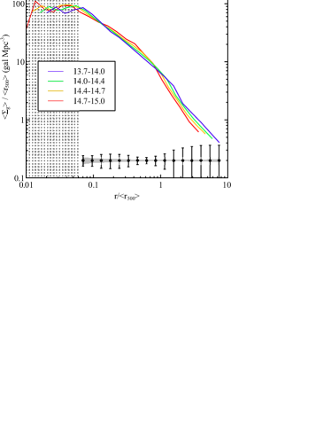
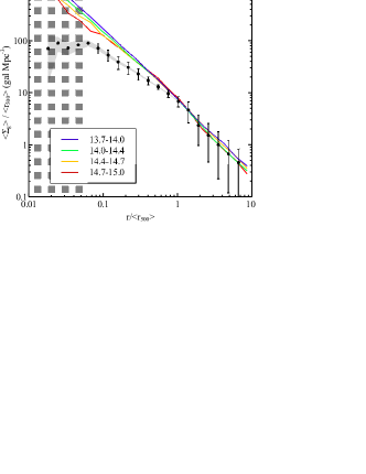
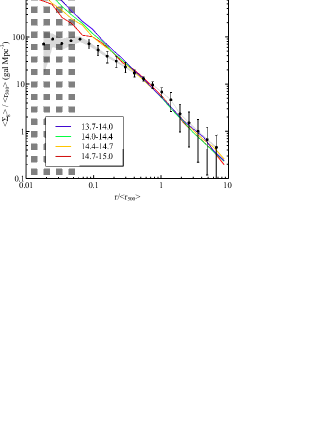
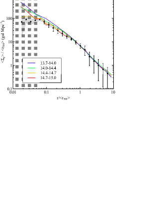
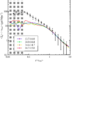
In order to study the mass-dependence of the satellite profiles we have split the sample into four bins ranging from to . The radial profiles (Figure 5) are obtained according to the method described in Section 4.1. In the Figure, the shaded (dotted) region corresponds to the region in physical space strongly affected by the BCG obscuration effects modelled in Section 4.2. As expected, the radial profile of the higher mass bins have a larger normalisation than the lower mass bins. This is due to the underlying mass-richness relation (Equation 3).

The choice of the four mass bins is motivated by the degree of scatter in the mass-richness relation (Figure 1). Ideally, one would like to divide the sample into multiple mass bins. However, the situation is made more complicated by the fact that the mass function of haloes is not uniform (right panel Figure 1), and also that there is potentially significant scatter of halo masses between bins. The choice of bin size is therefore a trade-off between needing enough bins to probe the physics of cluster formation which varies as a function of mass, and having bins wide enough to not have significant mass overlap due to mass measurement errors.
We can model the degree of scatter between the mass bins by making use of the mock cluster simulations described in Section 3.5.2. The mock clusters are analysed, and mass estimates are obtained according to the prescription in Sections 3.2 & 3.3. For a given input cluster mass, the recovered mass distribution from the simulation resembles a Gaussian about the input value, with a small degree of assymmetry owing to the nature of the Poisson process. To measure the effect of scatter between bins, we first model the scatter at the centre of a mass bin and convolve the recovered distribution with a square kernel with width equal to the size of the bin. This convolution widens the initial Gaussian, which represents the fact that the true cluster mass distribution is not entirely located at the centre of the bin. A further convolution is then required to account for shape of the cluster mass function (see right panel Figure 1), which is not uniform across each mass bin. The extra convolution causes the centre of the widened Gaussian to be offset to the left of the bin. This effect is more pronounced in the higher mass bins as the mass function is steeper. The resulting bin-to-bin scatter is shown in Figure 6. The lowest mass bin is strongly affected by the inclusion of real groups and clusters with true masses below the mass limit. This effect corresponds to 50 per cent contamination for the lowest mass bin, 5 per cent for the second lowest bin and is negligible for the higher mass bins. Despite the presence of significant scatter between mass bins (particularly at the lowest halo masses), distinct mass distributions within these four bins can be clearly seen. We can therefore be reasonably confident that any changes in shape seen in the radial profiles as a function of halo mass are real.

It has been known for some time that the dark matter mass density profiles look self-similar, i.e. no strong change in shape of the profile as a function of mass, (e.g. Navarro et al., 1997): if the radial coordinate in the profile is scaled by a characteristic radius, e.g., the virial radius, the resulting density distributions for systems with different total mass appear nearly identical101010They are not exactly identical because lower mass systems are slightly more concentrated than higher mass systems, which reflects the fact that lower mass systems collapsed earlier on average at a time when the background density of the Universe was higher.. It is interesting to see whether or not such self-similarity also holds for the satellite galaxy radial profiles.
We produce scaled radial satellite profiles by dividing both the distance and the number density by (the latter is required since is a surface number density therefore we must take into account that more massive objects have larger line-of-sight lengths in physical units). The stacked profiles are normalized by the mean value of for the four mass bins we consider. The mean value of is calculated as
| (7) |
where is the critical density of the universe at the redshift of the cluster, and is the mean mass in a given mass bin.
Figure 7 shows these scaled satellite profiles for the four mass bins considered. Remarkably, this scaling procedure removes most of the mass dependence in the satellite density distributions. Only a small residual difference remains in that the radial profiles of lower mass haloes appear to be slightly more peaked compared to those of the high mass clusters.

5.2 Satellite concentration
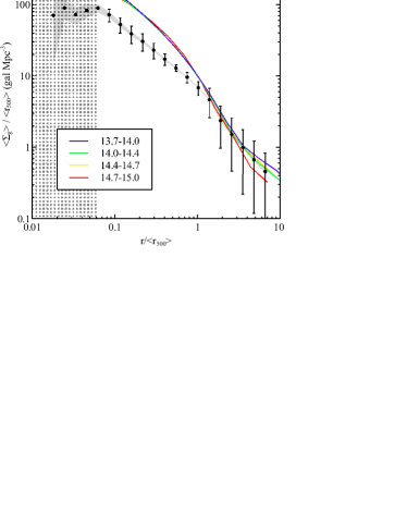
How well do satellites trace the underlying dark matter distribution? We can test whether the satellite behaviour is matched by the overall dark matter halo density distribution by looking at the projected dark matter density profiles from the Millenium Simulation (Springel et al., 2005). We select haloes in the same mass bins as the observations and create density profiles as a function of . The DM simulation profiles are arbitrarily normalised by multiplying them by a constant factor so that the profile corresponding to the [14.0-14.4] halo mass bin passes through the observed galaxy profile at (right panel of Fig. 7). As expected, the dark matter profiles are nearly self-similar. Interestingly, the dark matter profiles exhibit the same shape dependence as a function of mass as the satellite profiles (i.e. slightly more peaked at lower mass). This dark matter shape change is well documented in terms of the mass-concentration relationship in N-body simulations (Navarro et al., 1997; Bullock et al., 2001; Duffy et al., 2008; Gao et al., 2008), in which the lower mass haloes appear more concentrated compared to the high mass ones. This concentration dependence is thought to be due to the fact that more massive haloes collapse at a later cosmic time, where the background density of the universe is lower. It is not immediately obvious, though, that the satellites should preserve this trend, since presumably a large fraction of the satellites we see in orbit today were accreted not that long ago. The fact that the overall shapes of the satellite profiles are systematically different from the dark matter but that both are individually nearly self-similar is therefore quite intriguing.
We can quantify the difference in the shapes of the dark matter and the satellite density distributions by measuring their concentrations as described by the NFW profile (Figure 8). We fit the projected NFW profile (Bartelmann, 1996) to the satellite density profiles over the radial region . Figure 8 shows the obvious drop in halo concentration as a function of mass. The best-fit power-law relation of Gao et al. (2008), which was derived from fitting over a much wider range of halo masses, is over-plotted for comparison111111The small discrepancy between our derived mass-concentration relation for the simulated clusters and the best-fit power-law relation of Gao et al. (2008) may be the result of those authors fitting over a wider range of halo masses. Another difference is that our concentrations are derived by fitting to the projected surface mass density profiles, rather than to 3D density profiles.. One of the most striking observations is that the concentration of satellites is roughly a factor of two smaller than the dark matter across the full range of halo masses we have explored.
This systematic difference between the projected DM and galaxy radial distributions is generally consistent with the findings of previous studies. For example, Lin et al. (2004) in their study of 2MASS clusters in the K-band, find that the distribution of satellites has the mean concentration of 2.9. Additionally, two separate analyses of the CNOC clusters by Carlberg et al. (1997) and van der Marel et al. (2000) find the concentrations of 3.7 and 4.2 respectively. Although our concentrations are roughly a factor of 1.5 lower than these studies, we find a general qualitative agreement in that we see a relatively shallow dependence of the concentration on the halo mass. This shallow dependence is apparently discordant with the findings of Hansen et al. (2005) and Chen et al. (2006), who find that the concentration is a very strong function of optical richness. It is likely that this difference can be attributed to the differing characteristic radii used to scale the radial coordinates of the profiles (see the discussion in Section 1). Namely, Hansen et al. (2005) define their characteristic radii () with respect to the background density of galaxies, whereas our characteristic radii are defined with respect to the critical density of the Universe from X-ray measurements (see Equation 7). Indeed, using clusters in common between our catalog and that of the MaxBCG catalog, we find a scaling of , which accounts for the steep richness dependence of their derived concentrations.
Finally, a possible explanation for the offset between dark matter and satellite concentration is the fact that the galactic subhaloes are strongly affected by tidal evolution and merging process within the inner regions of the cluster (Nagai & Kravtsov, 2005; Chen et al., 2006). We will investigate the physics of subhalo disruption and merging in the context of semi-analytic galaxy formation models in Section 6.
5.3 Satellite profile shape as a function of other properties
Since the radial distribution of satellite galaxies does not vary strongly with halo mass, we can combine all galaxies into one cluster mass bin, ranging from to , and investigate the dependence of the profile (particularly its shape) on other properties. We now investigate whether the stacked radial profiles of satellite galaxies depend on redshift, BCG luminosity (or BCG luminosity fraction), and the luminosity and colour of the satellites themselves.
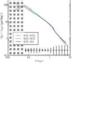
5.3.1 Redshift
Splitting the sample according to cluster redshift reveals a small change in the shape of the derived radial distribution (Fig. 9 (a)). In particular, within , the profile is slightly shallower in our lowest redshift bin with respect to that of the intermediate and high redshift bins. Beyond this radius, the shape and normalisation of the profiles in all three redshift bins are consistent with no evolution.
For reference, cosmological N-body simulations predict that the concentration should increase with decreasing redshift for a cluster of fixed mass (see, e.g., Duffy et al. 2008). However, over the relatively narrow range of redshift that we probe here, the DM concentration for a cluster of fixed mass would only vary by according to Duffy et al. (2008). In any case, it is not immediately obvious that the shape of the galaxy and DM radial distributions should evolve by the same amount or even in the same sense. Indeed, dynamical friction and tidal stripping/disruption could plausibly act to reduce the concentration of the satellite distribution (for clusters of fixed mass) over cosmic time.
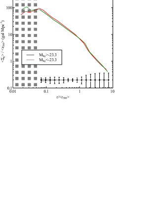
5.3.2 BCG luminosity
Splitting the sample according to relatively faint/bright BCGs (about the median BCG magnitude of ), reveals a small (but statistically significant within the Poisson error bars) difference between the two samples (panel (b) of Figure 9). Naively speaking, we might expect to see a central decrement in the satellite profiles for clusters with brighter than average BCGs (assuming the BCG is built from cannabalizing satellites). However, the observed trend actually goes the other way. A more mundane explanation for the trend is that there is a known dependence (albeit a relatively weak one) on the luminosity of the BCG and total cluster mass. When we split the sample based on BCG fraction (ratio of BCG luminosity to the background-subtracted cluster luminosity within 1 Mpc), the shape dependence of the satellite profiles all but disappears. We therefore find that when the halo mass dependence of the BCG luminosity is taken out, there is no obvious dependence of the satellite radial distribution on BCG luminosity.
(a)
 (b)
(b)
(c)
 (d)
(d)
5.3.3 Satellite luminosities
We turn our attention now to the brightness of the satellites themselves and investigate the dependence of the shape of the profile in four satellite luminosity bins over the range (panel (c) of Figure 9). We find that the concentration of satellites falls slightly as their brightness increases. This is opposite to the finding of Lin & Mohr (2004) and Chen et al. (2006) who find that the fainter satellites show a small dip in the central regions relative to the bright satellites. However, these studies only find a very small difference between faint/bright satellites and also stack a far fewer number of clusters than the number we present in this study.
Our results imply that the dwarf-to-giant ratio (DGR - the ratio of faint-to-bright galaxies), increases into the centre of the halo. This conclusion is in qualitative agreement with the work of Zabludoff & Mulchaey (2000), who find that the DGR decreases with halocentric radius albeit in a sample of lower masses and smaller redshifts than probed in this work. Zabludoff & Mulchaey (2000) propose a number of scenarios to explain the behaviour of the DGR with radius, particularly that brighter and more massive galaxies are subject to larger amounts of dynamical friction and thus more frequently merge with the BCG than their fainter counterparts. This effect leads to a deficiency of bright, massive galaxies in the centre of the halo. Our results would therefore suggest that such a mechanism may occur in the high mass end of clusters as well as in the poorer groups looked at by Zabludoff & Mulchaey (2000).
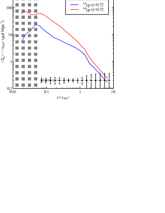
5.3.4 Satellite colours
A split of the satellite profile stacks into red and blue satellites (done about the median colour121212k-corrected to redshift zero. of ) yields a striking difference between their profile shapes. An impressive deficit131313It is worth noting that the slight rise at in the profile of blue galaxies could be an artifact possibly caused by the differential effects of BCG obscuration for the red/blue galaxies. of blue satellites in the centre of the halo relative to red satellites is consistent with what is found by Collister & Lahav (2005), who observe that the profiles of red galaxies () are much more concentrated than those of blue galaxies () in a large sample of 2PIGG groups. This conclusion is echoed by Weinmann et al. (2006); Weinmann et al. (2009) who find that the early-type141414‘Early/late-type’ is a definition based on the star-formation rate of the galaxy, but observationally these are very strongly correlated with red/blue colour of galaxies. fraction of galaxies decreases with increasing halocentric radius, and vice-versa for late-types.
A couple of mechanisms commonly invoked to explain the red/blue behaviour are ram-pressure stripping and strangulation. Ram-pressure stripping (Gunn & Gott, 1972) causes rapid removal of cold gas, and strangulation (Balogh et al., 2000) occurs when satellites are deprived of their hot gas reservoir. Both processes will result in a supression of star formation in the satellite galaxies and can transform late-type galaxies (blue) into early-types (red). These processes which quench star-formation become more severe as we move towards the centre of the halo, which explains the large observed discrepancy between red and blue galaxies within .
(a)
 (b)
(b)
(c)
 (d)
(d)
6 Semi-Analytic models
We can attempt to shed some light on the observed behaviour of the satellites in clusters (Section 5), by comparing our results with predictions from semi-analytic models of galaxy formation. In particular, we extract projected number density profiles for the Bower et al. (2006), Font et al. (2008) and De Lucia & Blaizot (2007) models using the Millennium Simulation SQL database151515http://virgo.dur.ac.uk/. We select all clusters from snapshot for which , yielding a sample of over 3000 simulated clusters. To mimic the procedure used to derive the observed profiles, we extract galaxies within a 5 Mpc aperture centered on the position of the most bound particle (which should correspond to the location of the BCG), perform a statistical background subtraction using a randomly placed 5 Mpc aperture placed, and retain only galaxies with a absolute rest-frame r-band magnitude .
In Fig 10 we show the stacked satellite profiles in four mass bins (the same ones as in Fig. 9) for the 3 models, along with a single stacked observational profile comprised of all the clusters in the sample161616The limited dependence of observed satellite concentration on halo mass in Fig 8, implies that we can reasonably combine all clusters in the sample into a single universal observational profile for comparison with the models.. We will discuss the bottom right panel below.
Underlying the Bower et al. (2006), Font et al. (2008) and De Lucia & Blaizot (2007) models are the same friends-of-friends (FoF) and substructure catalogs, which were produced by running the Subfind algorithm (Springel et al. 2001) on the Millennium Simulation. There are some slight differences in the merger trees constructed from these catalogs by the Durham and Munich groups and significant differences in the implementation of baryonic physics (such as radiative cooling, stellar evolution, supernova feedback, AGN feedback and so on). In principle the models could therefore produce quite different results. However, it should be borne in mind that all three models have been tuned to match the global galaxy luminosity function. What this tuning effectively achieves is to assign approximately the correct amount of luminosity/stellar mass to the central galaxy of a given dark matter halo (i.e., similar to what is achieved by direct ‘abundance matching’, but without explicitly imposing a monatonic relation between luminosity/stellar mass and halo mass or a constant amount of scatter at fixed halo mass). Our expectation, therefore, is that all three models ought to be similar at large radii and should, at least roughly, reproduce the observed unscaled satellite profiles there, where the effects of tidal evolution and dynamical friction should be minimal. Note that the model and observed scaled radial profiles will only match in normalisation at large radii if our estimates of are accurate, since we are using empirical estimates of for the observed clusters and the true values of for the simulated systems. As can be seen in Fig 10 all three models have similar behaviour at large radii and approximately match the observed profiles both in terms of shape and (encouragingly) normalisation. There is also a lack of a strong halo mass dependence in shape/normalisation of the profiles from the models, exactly as observed.
Within differences between the models become apparent. In particular, the De Lucia & Blaizot (2007) profiles become noticeably flatter, in rough accordance with the observed profiles, whereas the Bower et al. (2006) and Font et al. (2008) profiles show a smaller degree of flattening. At first sight, this may seem suprising, as all three models use the FoF and substructure catalogs. But note the difference between the models originates from differences in the treatment of satellite galaxies when the subhalo to which that galaxy belonged is no longer identified by Subfind . Subhaloes can be ‘lost’ either because they have been completely tidally disrupted or because the substructure finding algorithm has failed to find them. In Fig 10 (d) we show the profiles derived from the De Lucia & Blaizot (2007) model when only satellite galaxies with still existing subhaloes are included. This is equivalent to assuming that whenever a subhalo is lost the galaxy within it is completely destroyed. Here we see a very strong break in the profiles within , which is in obvious discord with the observations. The interesting implication of this experiment is that tidal disruption of satellites galaxies is much less efficient than the disruption of their surrounding dark matter subhalos171717Here we are making the assumption that the substructure finders are able to find most self-gravitating dark matter haloes..
In all three models when a satellite galaxy loses its dark matter subhalo the position of the satellite galaxy is assigned by using the current position of the most bound dark matter particle of the subhalo at the time the subhalo was last identified. This procedure cannot be followed indefinitely, of course, as no merging would take place with the central galaxy, since a single dark matter particle does not experience dynamical friction and therefore will not sink to the center. Therefore, what is done is to calculate a dynamical friction merger timescale, , for the satellite galaxy. This timescale is calculated differently in the Durham and Munich models. The Durham models use a timescale that is proportional to the original formation of Chandrasekhar (1943) (see Cole et al. 2000 for details) and depends on the main halo mass, the mass of the satellite, and orbital energy and angular momentum of the satellite. We note here that the mass of the satellite that is used is the total mass (gas+stars+dark matter) at the time of virial crossing of the main halo, rather than the time the subhalo was last identified. Also, the distribution of initial orbital parameters of infalling satellites (at virial crossing) is adopted from a fit to the cosmological simualtions of Tormen (1997) rather than using the orbital parameters of the satellites in the Millennium Simulation (we note, however, that a newer version of the GALFORM code allows for this possibility). The constant of proportionality, which is of order unity, is treated as a free parameter and varied to improve the match to the break in the galaxy luminosity function. Both the Bower et al. (2006) and Font et al. (2008) models use the same constant of proportionality. The Munich model, by contrast, uses the properties of the satellite (i.e., its mass and distance from the center) at the time its subhalo was last identified, which should be better, but their timescale calculation lacks any dependence on the orbital parameters, which should be relevant. There is also a constant of proportionality in the merger timescale in the Munich model, which De Lucia & Blaizot (2007) have tuned to improve the match to the break in the luminosity function.
Once a satellite galaxy has been in orbit for a time equal to the merger timescale181818Note the ‘clock’ starts ticking at different times for the Durham and Munich models. It starts at virial crossing for the Durham models and at the time the subhalo was last identified for the Munich model. the satellite is removed from the catalog and its mass is added to the central galaxy. Note that none of the models take into account mass loss due to tidal forces over the course of this merger timescale.
The larger degree of flattening of the profiles from the De Lucia & Blaizot (2007) model would suggest a generally shorter merger timescale than that which is being adopted in the Bower et al. (2006) and Font et al. (2008). Why this is the case is difficult to ascertain, given the large differences in the way in which these studies calculate this timescale. Recently, Jiang et al. (2008) and Boylan-Kolchin et al. (2008) used detailed numerical simulations to show that the current implementations of the dynamical friction merger timescale in the semi-analytic models do not accurately reproduce the true merger timescale from the simulations, in that they tend to underestimate the timescale for low mass satellites and overestimate it for massive satellites. This is likely due to a failure of a number of assumptions, including the neglect of mass loss (see Benson (2010) for further discussion).
In reality, the flattening of the satellites radial profiles is likely to be due to a combination of merging with the central galaxy and tidal mass loss of the satellites as they orbit about cluster. The fact that galaxy clusters contain detectable amounts of intra-cluster light (ICL) (see, e.g., Gonzalez et al. 2005; Zibetti et al. 2005) demonstrates that the latter mechanism has to be taking place as well. Disentangling these two processes relies upon understanding the complex interplay between the satellite profiles, the BCG luminosities and the ICL. In a forthcoming study (Koposov et al, in preparation) we will present self-consistent measure of ICL for the cluster sample presented here. In principle this should allow us to take a large jump towards understanding the complicated interplay between tidal stripping and satellite merging.
7 Conclusions
We have used the power of both spectroscopic and photometric datasets published as part of the SDSS DR7 to measure the satellite profiles of clusters with Luminous Red Galaxies (LRGs) at their centers. We take advantage of the large volume of the SDSS to probe a substantial range in halo mass (), and utilize the SDSS spectroscopic BCG sample to probe clusters out to a reasonably high redshift ().
Using the “anchor” sample of SDSS clusters with accurate X-ray temperature measurements we link the optical richness with the cluster’s extent and total mass . Armed with this robust measurement of halo mass, we have constructed a large catalogue of BCG clusters, which is highly pure and complete at halo masses of . The estimates of cluster mass are used to partition clusters in four bins according to the total amount of dark matter. In each mass bin, high signal-to-noise satellite profile stacks are produced. These reveal that accross all masses, the satellites are systematically less concentrated than the dark matter, roughly by a factor of two. Interestingly, in spite of the difference in shape between the galaxy and DM radial distributions, both exhibit a high degree of self-similarity (i.e. no strong change in shape of the profile as a function of mass). We find a strong evolution in the concentration of the satellite profile as a function of satellite brightness and colour and discuss physical mechanisms to explain this observed behaviour. We find only very weak dependencies of the satellite radial distribution on cluster redshift (over the range 0.15-0.4) or BCG luminosity.
We made a self-consistent comparison with a number of recent semi-analytic models of galaxy formation. We showed that: (1) beyond approx. current models are able to reproduce both the shape and normalisation of the satellite profiles; and (2) within the predicted profiles are sensitive to the details of the satellite-BCG merger timescale calculation. The former is a direct result of the models being tuned to match the global galaxy luminosity function combined with the assumption that the satellite galaxies do not suffer significant tidal stripping, even though their surrounding DM haloes can be removed through this process. The deviation within 0.3 r500 implies that the semi-analytic models have too long of a merger timescale and/or tidal stripping of the stellar component of galaxies, prior to merging with the BCG, is important (the effects of tidal stripping are not taken into account in the models that we have considered). The fact that groups and clusters demonstrably have non-neglibible stellar mass in a diffuse component (the ICL) indeed suggests that the latter process is relevant. In a forthcoming study we will present stacked measurements of the ICL for the cluster sample presented here. When combined with our measurements of the satellite population and the BCG it should be possible to gain a more complete understanding of the evolution/fate of the satellite population and could serve as a means to inform theoretical models on the efficacy of the tidal stripping and merging processes.
Acknowledgements
We thank the anonymous referee for helpful suggestions which improved the paper. We would like to thank Ann Zabludoff, Dennis Zaritsky, Paul Hewett and Manda Banerji for valuable discussions. JMB acknowledges the award of a STFC research studentship, whilst VB acknowledges financial support from the Royal Society. IGM acknowledges support from a Kavli Institute Fellowship at the University of Cambridge and a STFC Advanced Fellowship at the University of Birmingham. This work has made extensive use of the NumPy and SciPy Numerical Python packages and the Veusz plotting package. Funding for the Sloan Digital Sky Survey (SDSS) has been provided by the Alfred P. Sloan Foundation, the Participating Institutions, the National Aeronautics and Space Administration, the National Science Foundation, the US Department of Energy, the Japanese Monbukagakusho, and the Max Planck Society. The SDSS website is http://www.sdss.org/. The SDSS is managed by the Astrophysical Research Consortium (ARC) for the Participating Institutions. The Participating Institutions are The University of Chicago, Fermilab, the Institute for Advanced Study, the Japan Participation Group, The Johns Hopkins University, Los Alamos National Laboratory, the Max Planck Institute for Astronomy (MPIA), the Max Planck Institute for Astrophysics (MPA), New Mexico State University, the University of Pittsburgh, Princeton University, the United States Naval Observatory, and the University of Washington.
References
- Angulo et al. (2009) Angulo R. E., Lacey C. G., Baugh C. M., Frenk C. S., 2009, MNRAS, 399, 983
- Baldry et al. (2008) Baldry I. K., Glazebrook K., Driver S. P., 2008, MNRAS, 388, 945
- Balogh et al. (2000) Balogh M. L., Navarro J. F., Morris S. L., 2000, ApJ, 540, 113
- Bartelmann (1996) Bartelmann M., 1996, A&A, 313, 697
- Benson (2010) Benson A. J., 2010, Physics Reports, 495, 33
- Bertin & Arnouts (1996) Bertin E., Arnouts S., 1996, A&A, 117, 393
- Bildfell et al. (2008) Bildfell C., Hoekstra H., Babul A., Mahdavi A., 2008, MNRAS, 389, 1637
- Bode et al. (2001) Bode P., Ostriker J. P., Turok N., 2001, ApJ, 556, 93
- Bolton et al. (2008) Bolton A. S., Burles S., Koopmans L. V. E., Treu T., Gavazzi R., Moustakas L. A., Wayth R., Schlegel D. J., 2008, ApJ, 682, 964
- Bower et al. (2006) Bower R. G., Benson A. J., Malbon R., Helly J. C., Frenk C. S., Baugh C. M., Cole S., Lacey C. G., 2006, MNRAS, 370, 645
- Boylan-Kolchin et al. (2008) Boylan-Kolchin M., Ma C.-P., Quataert E., 2008, MNRAS, 383, 93
- Bullock et al. (2001) Bullock J. S., Kolatt T. S., Sigad Y., Somerville R. S., Kravtsov A. V., Klypin A. A., Primack J. R., Dekel A., 2001, MNRAS, 321, 559
- Bullock et al. (2000) Bullock J. S., Kravtsov A. V., Weinberg D. H., 2000, ApJ, 539, 517
- Carlberg et al. (1997) Carlberg R. G., Yee H. K. C., Ellingson E., 1997, ApJ, 478, 462
- Cavagnolo et al. (2009) Cavagnolo K. W., Donahue M., Voit G. M., Sun M., 2009, ApJS, 182, 12
- Chandrasekhar (1943) Chandrasekhar S., 1943, ApJ, 97, 255
- Chen et al. (2006) Chen J., Kravtsov A. V., Prada F., Sheldon E. S., Klypin A. A., Blanton M. R., Brinkmann J., Thakar A. R., 2006, ApJ, 647, 86
- Chilingarian et al. (2010) Chilingarian I. V., Melchior A.-L., Zolotukhin I. Y., 2010, MNRAS, 405, 1409
- Cole et al. (2000) Cole S., Lacey C. G., Baugh C. M., Frenk C. S., 2000, MNRAS, 319, 168
- Collister & Lahav (2005) Collister A. A., Lahav O., 2005, MNRAS, 361, 415
- Conroy et al. (2006) Conroy C., Wechsler R. H., Kravtsov A. V., 2006, ApJ, 647, 201
- Conroy et al. (2007) Conroy C., Wechsler R. H., Kravtsov A. V., 2007, ApJ, 668, 826
- Crawford et al. (1999) Crawford C. S., Allen S. W., Ebeling H., Edge A. C., Fabian A. C., 1999, MNRAS, 306, 857
- Croton et al. (2006) Croton D. J., Springel V., White S. D. M., De Lucia G., Frenk C. S., Gao L., Jenkins A., Kauffmann G., Navarro J. F., Yoshida N., 2006, MNRAS, 365, 11
- De Lucia & Blaizot (2007) De Lucia G., Blaizot J., 2007, MNRAS, 375, 2
- Dolag et al. (2009) Dolag K., Borgani S., Murante G., Springel V., 2009, MNRAS, 399, 497
- Duffy et al. (2008) Duffy A. R., Schaye J., Kay S. T., Dalla Vecchia C., 2008, MNRAS, 390, L64
- Eisenstein et al. (2001) Eisenstein D. J., et al., 2001, AJ, 122, 2267
- Font et al. (2008) Font A. S., Bower R. G., McCarthy I. G., Benson A. J., Frenk C. S., Helly J. C., Lacey C. G., Baugh C. M., Cole S., 2008, MNRAS, 389, 1619
- Gao et al. (2008) Gao L., Navarro J. F., Cole S., Frenk C. S., White S. D. M., Springel V., Jenkins A., Neto A. F., 2008, MNRAS, 387, 536
- Gonzalez et al. (2005) Gonzalez A. H., Zabludoff A. I., Zaritsky D., 2005, ApJ, 618, 195
- Gonzalez et al. (2007) Gonzalez A. H., Zaritsky D., Zabludoff A. I., 2007, ApJ, 666, 147
- Gunn & Gott (1972) Gunn J. E., Gott III J. R., 1972, ApJ, 176, 1
- Guo et al. (2010) Guo Q., White S., Li C., Boylan-Kolchin M., 2010, MNRAS, 404, 1111
- Haas et al. (2011) Haas M. R., Schaye J., Jeeson-Daniel A., 2011, ArXiv e-prints
- Hansen et al. (2005) Hansen S. M., McKay T. A., Wechsler R. H., Annis J., Sheldon E. S., Kimball A., 2005, ApJ, 633, 122
- Hao et al. (2010) Hao J., et al., 2010, ApJS, 191, 254
- Hogg et al. (2010) Hogg D. W., Bovy J., Lang D., 2010, ArXiv e-prints
- Horner (2001) Horner D. J., 2001, PhD thesis, University of Maryland College Park
- Jiang et al. (2008) Jiang C. Y., Jing Y. P., Faltenbacher A., Lin W. P., Li C., 2008, ApJ, 675, 1095
- Kamionkowski & Liddle (2000) Kamionkowski M., Liddle A. R., 2000, Physical Review Letters, 84, 4525
- Klypin et al. (1999) Klypin A., Kravtsov A. V., Valenzuela O., Prada F., 1999, ApJ, 522, 82
- Klypin et al. (2010) Klypin A., Trujillo-Gomez S., Primack J., 2010, ArXiv e-prints
- Koester et al. (2007) Koester B. P., et al., 2007, ApJ, 660, 239
- Koposov & Bartunov (2006) Koposov S., Bartunov O., 2006, 351, 735
- Koposov et al. (2009) Koposov S. E., Yoo J., Rix H.-W., Weinberg D. H., Macciò A. V., Escudé J. M., 2009, ApJ, 696, 2179
- Kravtsov et al. (2004) Kravtsov A. V., Berlind A. A., Wechsler R. H., Klypin A. A., Gottlöber S., Allgood B., Primack J. R., 2004, ApJ, 609, 35
- Kravtsov et al. (2004) Kravtsov A. V., Gnedin O. Y., Klypin A. A., 2004, ApJ, 609, 482
- Lin & Mohr (2004) Lin Y., Mohr J. J., 2004, ApJ, 617, 879
- Lin et al. (2004) Lin Y., Mohr J. J., Stanford S. A., 2004, ApJ, 610, 745
- Lupton et al. (2001) Lupton R., Gunn J. E., Ivezić Z., Knapp G. R., Kent S., 2001, 238, 269
- Maughan et al. (2008) Maughan B. J., Jones C., Forman W., Van Speybroeck L., 2008, ApJS, 174, 117
- Moore et al. (1999) Moore B., Ghigna S., Governato F., Lake G., Quinn T., Stadel J., Tozzi P., 1999, ApJL, 524, L19
- Moster et al. (2010) Moster B. P., Somerville R. S., Maulbetsch C., van den Bosch F. C., Macciò A. V., Naab T., Oser L., 2010, ApJ, 710, 903
- Mulchaey et al. (2003) Mulchaey J. S., Davis D. S., Mushotzky R. F., Burstein D., 2003, ApJS, 145, 39
- Muzzin et al. (2007) Muzzin A., Yee H. K. C., Hall P. B., Ellingson E., Lin H., 2007, ApJ, 659, 1106
- Nagai & Kravtsov (2005) Nagai D., Kravtsov A. V., 2005, ApJ, 618, 557
- Navarro et al. (1997) Navarro J. F., Frenk C. S., White S. D. M., 1997, ApJ, 490, 493
- Osmond & Ponman (2004) Osmond J. P. F., Ponman T. J., 2004, MNRAS, 350, 1511
- Rawle et al. (2012) Rawle T. D., Edge A. C., Egami E., Rex M., Smith G. P., Altieri B., Fiedler A., Haines C. P., Pereira M. J., Pérez-González P. G., Portouw J., Valtchanov I., Walth G., van der Werf P. P., Zemcov M., 2012, ArXiv e-prints
- Sales et al. (2007) Sales L. V., Navarro J. F., Lambas D. G., White S. D. M., Croton D. J., 2007, MNRAS, 382, 1901
- Saro et al. (2006) Saro A., Borgani S., Tornatore L., Dolag K., Murante G., Biviano A., Calura F., Charlot S., 2006, MNRAS, 373, 397
- Shankar et al. (2006) Shankar F., Lapi A., Salucci P., De Zotti G., Danese L., 2006, ApJ, 643, 14
- Shaw et al. (2007) Shaw L. D., Weller J., Ostriker J. P., Bode P., 2007, ApJ, 659, 1082
- Skibba et al. (2010) Skibba R. A., van den Bosch F., Yang X., Mo H., More S., Fontanot F., 2010, 42, 330.02
- Somerville (2002) Somerville R. S., 2002, ApJL, 572, L23
- Spergel & Steinhardt (2000) Spergel D. N., Steinhardt P. J., 2000, Physical Review Letters, 84, 3760
- Springel et al. (2005) Springel V., et al., 2005, Nature, 435, 629
- Springel et al. (2001) Springel V., Yoshida N., White S. D. M., 2001, New A, 6, 79
- Sun et al. (2009) Sun M., Voit G. M., Donahue M., Jones C., Forman W., Vikhlinin A., 2009, ApJ, 693, 1142
- Szabo et al. (2011) Szabo T., Pierpaoli E., Dong F., Pipino A., Gunn J., 2011, ApJ, 736, 21
- Tojeiro & Percival (2010) Tojeiro R., Percival W. J., 2010, MNRAS, 405, 2534
- Tojeiro & Percival (2011) Tojeiro R., Percival W. J., 2011, ArXiv e-prints
- Tormen (1997) Tormen G., 1997, MNRAS, 290, 411
- Vale & Ostriker (2004) Vale A., Ostriker J. P., 2004, MNRAS, 353, 189
- van den Bosch et al. (2005) van den Bosch F. C., Yang X., Mo H. J., Norberg P., 2005, MNRAS, 356, 1233
- van der Marel et al. (2000) van der Marel R. P., Magorrian J., Carlberg R. G., Yee H. K. C., Ellingson E., 2000, AJ, 119, 2038
- Vikhlinin et al. (2006) Vikhlinin A., Kravtsov A., Forman W., Jones C., Markevitch M., Murray S. S., Van Speybroeck L., 2006, ApJ, 640, 691
- Voit (2005) Voit G. M., 2005, Advances in Space Research, 36, 701
- Voit et al. (2002) Voit G. M., Bryan G. L., Balogh M. L., Bower R. G., 2002, ApJ, 576, 601
- Weinmann et al. (2009) Weinmann S. M., Kauffmann G., van den Bosch F. C., Pasquali A., McIntosh D. H., Mo H., Yang X., Guo Y., 2009, MNRAS, 394, 1213
- Weinmann et al. (2006) Weinmann S. M., van den Bosch F. C., Yang X., Mo H. J., 2006, MNRAS, 366, 2
- Wen et al. (2009) Wen Z. L., Han J. L., Liu F. S., 2009, ApJS, 183, 197
- Yee & Ellingson (2003) Yee H. K. C., Ellingson E., 2003, ApJ, 585, 215
- Zabludoff & Mulchaey (2000) Zabludoff A. I., Mulchaey J. S., 2000, ApJ, 539, 136
- Zentner & Bullock (2003) Zentner A. R., Bullock J. S., 2003, ApJ, 598, 49
- Zibetti et al. (2005) Zibetti S., White S. D. M., Schneider D. P., Brinkmann J., 2005, MNRAS, 358, 949
Appendix A Linear model fitting
This describes the formalism from Hogg et al. (2010) for the fitting of a straight line model with slope and intercept , to data with two dimensional uncertainties.
The orthogonal displacement of each data point from the line is given by:
| (8) |
where is the individual data point, and is the unit vector orthogonal to the line given by:
| (9) |
Each data points covariance matrix is given by:
| (10) |
where the covariance matrix of horizontal and vertical measurement uncertainties corresponds to:
| (11) |
Appendix B MaxBCG radial profiles
Fig. 11 shows the raw unscaled satellite number density profiles for the MaxBCG clusters (Koester et al., 2007), in four mass bins. The profiles are very similar to those generated using the cluster sample described in this paper (Fig. 5).
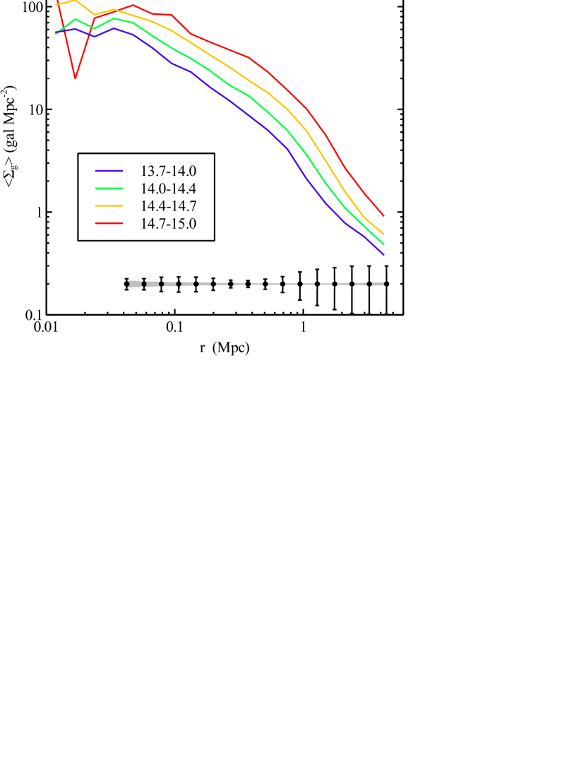
Appendix C Error modelling
In order to estimate the scatter in number density profiles we perform the following analysis. As described in the text we are interested in the scatter of the scaled surface density: as a function of log(R/R500). Our data consist of the measurements of the number of galaxies in circular annuli for different clusters and the corresponding measurements of the background galaxy density.
First we consider the expected number of galaxies in the -th bin of log(R/R500) for the galaxy cluster :
| (12) |
where is the area of the -th annulus for -th cluster, is the of the -th cluster, is a scaled density of galaxies in the cluster and is the background galaxy density. In the simplest scenario we would assume that is constant for all clusters, but in this case we will assume that the is Gaussian distributed with the mean and dispersion .
Now we can write the likelihood of the parameters given observed galaxies in the -th bin of the -th cluster and background galaxies observed in the random 5 Mpc radius field:
| (13) |
where the first term is Poisson probability of observing the objects given a certain density of galaxies (including background), the second term is the probability of having given the mean density and scatter , and the third term is essentially is Gaussian probability of the background measurement from the random 5 Mpc radius field. In our case we are not interested in the values of , so their are nuisance parameters for us and we can marginalize over them. Then the likelihood becomes only a function of :
| (14) |
The full likelihood for the -th bin of the profile is then obtained by multiplying the likelihoods for different clusters
| (15) |
We then maximize that likelihood with respect to the parameters for each radial bin, which gives as estimates of the mean and a scatter of the density profiles. For the error estimates of the parameters we use Hessian matrices numerically evaluated at the best-fit parameters.