Large current noise in nanoelectromechanical systems close to continuous mechanical instabilities

Abstract

We investigate the current noise of nanoelectromechanical systems close to a continuous mechanical instability. In the vicinity of the latter, the vibrational frequency of the nanomechanical system vanishes, rendering the system very sensitive to charge fluctuations and, hence, resulting in very large (super-Poissonian) current noise. Specifically, we consider a suspended single-electron transistor close to the Euler buckling instability. We show that such a system exhibits an exponential enhancement of the current noise when approaching the Euler instability which we explain in terms of telegraph noise.

I Introduction

Nanoelectromechanical systems (NEMS) in which a nanomechanical resonator is coupled to electronic degrees of freedom craig00_Science ; ekinc05_RSI ; poot11_preprint through, e.g., a single-electron transistor (SET), show spectacular effects stemming from the coupling of the mechanical part of the device to the electronic charge. These effects arise due to the reduced size of the nanoresonator, so that the backaction of the mechanical degree of freedom on the SET can have significant consequences for the transport properties. A prominent example is the low-bias current blockade that occurs in the Coulomb blockade regime when the nanoresonator is capacitively coupled to the SET. pisto07_PRB ; pisto08_PRB The presence of an extra electron with charge $-e<0$ on the central island forming a quantum dot on the suspended vibrating structure induces an electrostatic force $F_{\mathrm{e}}$ on the resonator, shifting the equilibrium position of the latter by an amount $F_{\mathrm{e}}/k$, with $k$ the spring constant of the oscillator (see Fig. 1). This induces a shift of the gate voltage $V_{\mathrm{g}}\sim F_{\mathrm{e}}^{2}/ek$ seen by the SET, and, hence, a blockade of the current through the device for bias voltages $V\lesssim F_{\mathrm{e}}^{2}/ek$. This phenomenon is the classical counterpart of the Franck-Condon blockade in molecular devices koch05_PRL ; koch06_PRB that has recently been observed in carbon nanotube-based resonators for high-energy longitudinal stretching modes. letur09_NaturePhysics For classical nanoresonators, the current blockade has, to the best of our knowledge, never been observed experimentally due to the relatively weak electromechanical coupling $F_{\mathrm{e}}$ to the low-energy bending modes of the suspended structure, although a precursor of this effect has been lately reported in the literature. steel09_Science ; lassa09_Science

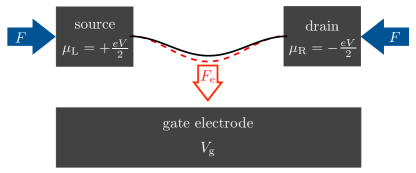
Figure 1: (Color online) Sketch of a suspended doubly clamped nanobeam forming a quantum dot (solid black line) connected via tunnel barriers to source and drain electrodes held at chemical potentials $\mu_{\mathrm{L}}$ and $\mu_{\mathrm{R}}$ by the bias voltage $V$. The lateral force $F$ compresses the nanobeam and induces the buckling instability. The beam is capacitively coupled to a metallic electrode kept at a gate voltage $V_{\mathrm{g}}$. This induces a stochastic force $F_{\mathrm{e}}$ that attracts the beam towards the gate electrode whenever the quantum dot is charged (dashed red line), inducing fluctuations of the nanobeam’s deflection and, in turn, fluctuations of the current through the device.

It has been recently shown weick11_PRB ; weick11b_PRB how one can enhance the classical current blockade by orders of magnitude by exploiting the well-known Euler buckling instability. landau Indeed, the spring constant $k$ (or equivalently, the vibrational frequency of the fundamental bending mode $\omega$) tends to zero when one brings the nanoresonator to the buckling instability with the help of a lateral compression force $F$ (see Fig. 1). Thus, the energy scale $F_{\mathrm{e}}^{2}/k$ at which the current blockade occurs dramatically increases, rendering this phenomenon potentially observable in future experiments.

It is the purpose of the present paper to investigate the current noise in the vicinity of a mechanical instability, using the Euler buckling instability as a paradigmatic model. We find that the current noise (which contains valuable information about the dynamics of the nanomechanical system armou04_PRB ; blant04_PRL ; usman07_PRB ; pisto04_PRB ; novot04_PRL ; donar05_NJP ; flind05_EPL ) is strongly enhanced in the vicinity of the Euler instability. The underlying source of noise arises from the stochastic nature of the charge transfer processes. These are producing a current-induced stochastic force acting on the mechanical degrees of freedom, consisting of current-induced (conservative and nonconservative) averages as well as a fluctuating force. pisto07_PRB ; pisto08_PRB ; weick11_PRB ; weick11b_PRB ; blant04_PRL ; mozyr06_PRB ; husse10_PRB ; nocer11_PRB ; bode11_PRL ; bode11_preprint ; weick10_PRB Hence, the deflection of the nanotube exhibits a Langevin dynamics which, due to the backaction of the nanoresonator on the SET, produces large super-Poissonian current noise. armou04_PRB ; usman07_PRB ; pisto08_PRB ; blant04_PRL ; novot04_PRL ; donar05_NJP ; flind05_EPL This effect is particularly strong close to the Euler buckling instability, where the nanoresonator becomes extremely soft ($k\to 0$).

Our theoretical approach employs a nonequilibrium Born-Oppenheimer approximation, pisto07_PRB ; pisto08_PRB ; blant04_PRL ; mozyr06_PRB ; husse10_PRB ; nocer11_PRB ; bode11_PRL ; bode11_preprint which exploits the separation of timescales between fast electronic and slow mechanical degrees of freedom. This leads to an effective stochastic description of the nanoresonator in terms of a Langevin equation. This approach becomes asymptotically exact in the vicinity of the mechanical instability where $\omega\to 0$. weick10_PRB ; weick11_PRB ; weick11b_PRB

The paper is organized as follows: Our model and the effective Langevin description of the nanoresonator deflection is presented in Sec. II. In Sec. III, we briefly recall the main results of Ref. weick11_PRB, for the current-voltage characteristics of the system that are essential for the understanding of our numerical investigation of the current noise presented in Sec. IV. In Sec. V, we detail the role played by thermal fluctuations on the current noise and propose an analytical model based on telegraph noise that reproduces most of our numerical findings. We present in Sec. VI the role played by the full nonequilibrium fluctuations on the noise before we conclude in Sec. VII.

II Model

The model we adopt is the same as in Ref. weick11_PRB, and we briefly recall it here for the convenience of the reader. The setup (see Fig. 1) consists of a quantum dot embedded in a suspended nanobeam connected via tunnel barriers to source and drain leads. A lateral compression force $F$ exerted on the nanobeam brings it to the Euler buckling instability when $F$ approaches the critical force $F_{\mathrm{c}}$. The gate electrode induces an electromechanical coupling between the bending modes of the tube and the charge state of the dot proportional to the electrostatic force $F_{\mathrm{e}}$. The Hamiltonian of the system reads

$$H=H_{\mathrm{vib}}+H_{\mathrm{SET}}+H_{\mathrm{c}},$$ (1)

where $H_{\mathrm{vib}}$ describes the oscillating modes of the nanobeam, $H_{\mathrm{SET}}$ the single-electron transistor, and $H_{\mathrm{c}}$ the coupling between vibrational modes and electronic degrees of freedom.

At the Euler buckling instability ($F=F_{\mathrm{c}}$), the frequency of the fundamental bending mode

$$\omega=\omega_{0}\sqrt{-\delta},\qquad\delta=\frac{F}{F_{\mathrm{c}}}-1$$ (2)

vanishes, landau $\omega_{0}$ being the frequency of that mode for $F=0$, while all higher energy modes have a finite frequency. At sufficiently low temperatures, we thus only consider the fundamental bending mode and write weick10_PRB ; weick11b_PRB ; weick11_PRB ; carr01_PRB ; werne04_EPL ; peano06_NJP ; savel06_NJP

$$H_{\mathrm{vib}}=\frac{P^{2}}{2m}+\frac{m\omega^{2}}{2}X^{2}+\frac{\alpha}{4}X^{4}$$ (3)

for the vibrational part of the Hamiltonian (1). Here, $X$ is the deflection of the tube and $P$ its associated canonical momentum with effective mass $m$. In Eq. (3), the quartic term proportional to $\alpha>0$ ensures the stability of the system for $F>F_{\mathrm{c}}$ ($\omega^{2}<0$), where the beam buckles into one of the two metastable positions at $X=\pm\sqrt{-m\omega^{2}/\alpha}$. For $F<F_{\mathrm{c}}$ ($\omega^{2}>0$), the beam remains flat.

We model the SET by a single-level quantum dot with orbital energy $\epsilon_{\mathrm{d}}$ connected via tunnel barriers to left (L) and right (R) leads held at chemical potential $\mu_{\mathrm{L}}$ and $\mu_{\mathrm{R}}$, respectively. The SET Hamiltonian reads $H_{\mathrm{SET}}=H_{\mathrm{dot}}+H_{\mathrm{leads}}+H_{\mathrm{tun}}$, where the dot Hamiltonian $H_{\mathrm{dot}}=(\epsilon_{\mathrm{d}}-e\bar{V}_{\mathrm{g}})n_{\mathrm{d}}+Un_{\mathrm{d}}(n_{\mathrm{d}}-1)/2$ is expressed in terms of $n_{\mathrm{d}}=d^{\dagger}d$, $d$ annihilating an electron on the dot. Here, $\bar{V}_{\mathrm{g}}$ is the (effective) applied gate voltage. The intradot Coulomb repulsion is denoted by $U$ and is assumed to be the largest energy scale in the problem, thus preventing double occupancy of the dot. The Hamiltonian for the (spinless) electrons with energy $\epsilon_{k}$ and momentum $k$ in the two leads (annihilated by the operator $c_{ka}$, $a=\mathrm{L,R}$) is written as $H_{\mathrm{leads}}=\sum_{ka}(\epsilon_{k}-\mu_{a})c_{ka}^{\dagger}c_{ka}^{\phantom{\dagger}}$. Finally, tunneling between dot and leads is accounted for by the Hamiltonian $H_{\mathrm{tun}}=\sum_{ka}(t_{a}c_{ka}^{\dagger}d+\mathrm{h.c.})$, with $t_{a}$ the tunneling amplitude between the dot and lead $a$. In the remainder of this paper, we assume the temperature $T$ to be much larger than the tunneling-induced width $\Gamma=\sum_{a}\Gamma_{a}$ of the dot orbital (sequential tunneling regime). This weak-coupling assumption should not qualitatively change our results for the low-frequency current noise, as it is the case for the $I$-$V$ characteristics which is qualitatively the same in the sequential weick11_PRB and cotunneling weick11b_PRB regimes. Moreover, we consider for simplicity symmetric voltage drops ($\mu_{\mathrm{L}}=-\mu_{\mathrm{R}}=eV/2$) and symmetric coupling to the leads ($\Gamma_{\mathrm{L}}=\Gamma_{\mathrm{R}}=\Gamma/2$).

The coupling Hamiltonian between vibrational and electronic degrees of freedom entering Eq. (1),

$$H_{\mathrm{c}}=F_{\mathrm{e}}Xn_{\mathrm{d}},$$ (4)

arises due to the capacitive coupling between the gate electrode and the nanobeam when the latter is charged with one extra electron. sapma03_PRB ; steel09_Science ; lassa09_Science Since the dot occupation $n_{\mathrm{d}}$ is a stochastic variable (taking values 0 and 1 in our model), the coupling (4) produces a random electrostatic force with magnitude $F_{\mathrm{e}}$ on the nanobeam (see Fig. 1).

As $\omega\to 0$ close to the buckling instability, the oscillator becomes classical ($\hbar\omega\ll k_{\mathrm{B}}T$) and slow compared to the electronic degrees of freedom ($\omega\ll\Gamma$). This justifies a nonequilibrium Born-Oppenheimer approximation, blant04_PRL ; weick10_PRB ; weick11_PRB ; weick11b_PRB ; mozyr06_PRB ; husse10_PRB ; nocer11_PRB ; bode11_PRL ; bode11_preprint in which the vibrational dynamics is characterized by a Langevin process with white noise,

$$\frac{\mathrm{d}^{2}x}{\mathrm{d}\tau^{2}}+\left[\gamma(x)+\gamma_{\mathrm{e}}\right]\frac{\mathrm{d}x}{\mathrm{d}\tau}=f_{\mathrm{eff}}(x)+\xi(x,\tau).$$ (5)

Here and in what follows, we use reduced units $x=X/\ell$, $p=P/m\omega_{0}\ell$ and $\tau=\omega_{0}t$ in terms of the polaron shift $\ell=F_{\mathrm{e}}/m\omega_{0}^{2}$ and the relevant energy scale of the problem $E_{\mathrm{E}}^{0}=F_{\mathrm{e}}\ell$ (for more details, see Ref. weick11_PRB, ). In Eq. (5), the effective force acting on the nanobeam,

$$f_{\mathrm{eff}}(x)=\delta x-\tilde{\alpha}x^{3}-n_{0}(x),$$ (6)

with $\tilde{\alpha}=\alpha\ell^{4}/E_{\mathrm{E}}^{0}$, arises (i) from the bare vibrational Hamiltonian (3) and (ii) from the coupling between vibrational and electronic degrees of freedom (4). This current-induced force is proportional to the occupation of the dot for fixed $x$, which, in the sequential tunneling regime ($\hbar\Gamma\ll k_{\mathrm{B}}T$), is given by

$$n_{0}(x)=\frac{1}{2}\left[f_{\mathrm{L}}(x)+f_{\mathrm{R}}(x)\right],$$ (7)

with

$$f_{\mathrm{L/R}}(x)=\left[\exp{\left(\frac{x-v_{\mathrm{g}}\mp v/2}{\tilde{T}}\right)}+1\right]^{-1}$$ (8)

the Fermi function in the left and right leads, respectively. Here we introduced a reduced bias voltage $v=eV/E_{\mathrm{E}}^{0}$, gate voltage $v_{\mathrm{g}}=(e\bar{V}_{\mathrm{g}}-\epsilon_{\mathrm{d}})/E_{\mathrm{E}}^{0}$, and temperature $\tilde{T}=k_{\mathrm{B}}T/E_{\mathrm{E}}^{0}$. The charge fluctuations on the quantum dot induce a fluctuating force $\xi(x,\tau)$ in the Langevin equation (5), with average $\langle\xi(x,\tau)\rangle=0$ and white-noise correlator $\langle\xi(x,\tau)\xi(x,\tau^{\prime})\rangle=[d(x)+2\gamma_{\mathrm{e}}\tilde{T}]\delta(\tau-\tau^{\prime})$. Here, the current-induced fluctuation is given by pisto07_PRB ; weick11_PRB

$$d(x)=\frac{2\omega_{0}}{\Gamma}n_{0}(x)\left[1-n_{0}(x)\right],$$ (9)

and the extrinsic damping constant $\gamma_{\mathrm{e}}$ accounts for the finite quality factor $Q=1/\gamma_{\mathrm{e}}$ of the nanoresonator. Finally, retardation effects in the response of the resonator to the current flow lead to a current-induced dissipative force with friction coefficient pisto07_PRB ; weick11_PRB

$$\gamma(x)=-\frac{\omega_{0}}{\Gamma}\frac{\partial}{\partial x}n_{0}(x).$$ (10)

The Langevin equation (5) is equivalent to the Fokker-Planck equation zwanzig

$$\frac{\partial}{\partial\tau}\mathcal{P}(x,p,\tau)={\mathcal{L}}\mathcal{P}(x,p,\tau)$$ (11)

for the probability distribution $\mathcal{P}(x,p,\tau)$ that the nanobeam is at phase-space point $(x,p)$ at time $\tau$. In Eq. (11), the Fokker-Planck operator is defined as

$${\mathcal{L}}= -p\frac{\partial}{\partial x}-f_{\mathrm{eff}}(x)\frac{\partial}{\partial p}+\left[\gamma(x)+\gamma_{\mathrm{e}}\right]\frac{\partial}{\partial p}p$$

$$+\left[\frac{d(x)}{2}+\gamma_{\mathrm{e}}\tilde{T}\right]\frac{\partial^{2}}{\partial p^{2}}.$$ (12)

Solving the Fokker-Planck equation (11) [or equivalently the Langevin equation (5)] gives access to both the dynamics of the vibrational mode of the nanoresonator and the resulting transport properties of the device, such as its $I$-$V$ characteristics (see Sec. III) and its noise power spectrum (see Secs. IV, V and VI).

III Current blockade

Due to the separation of timescales between slow vibrational motion and fast electronic dynamics, the average current

$$I=\int\mathrm{d}x\mathrm{d}p\;\mathcal{P}_{\mathrm{st}}(x,p)\mathcal{I}(x)$$ (13)

is obtained by averaging the quasistationary current

$$\mathcal{I}(x)=\frac{e\Gamma}{4}\left[f_{\mathrm{L}}(x)-f_{\mathrm{R}}(x)\right]$$ (14)

for fixed deflection $x$ over the stationary solution $\mathcal{P}_{\mathrm{st}}$ of the Fokker-Planck equation (11).

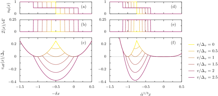
Figure 2: (Color online) Zero temperature (a,d) average occupation of the dot for fixed $x$ [Eq. (7)], (b,e) quasistationary current [Eq. (14)] and (c,f) effective potential [Eq. (15)], (a,b,c) far below the Euler instability ($-\delta\gg\tilde{\alpha}^{1/3}$) and (d,e,f) at the instability ($\delta=0$) for increasing bias voltages and for a gate voltage $v_{\mathrm{g}}=v_{\mathrm{g}}^{\mathrm{min}}$ [cf. Eq. (17)].

The classical current blockade phenomenon weick11_PRB ; pisto07_PRB can be understood in terms of the effective potential

$$v_{\mathrm{eff}}(x)=-\frac{\delta x^{2}}{2}+\frac{\tilde{\alpha}x^{4}}{4}+x+\frac{\tilde{T}}{2}\ln{\big{(}f_{\mathrm{L}}(x)f_{\mathrm{R}}(x)\big{)}}$$ (15)

associated to the effective force (6). The effective potential is shown in Fig. 2 for $\tilde{T}=0$ together with the average occupation of the dot (7) and the quasistationary current (14) for compression forces corresponding to the beam far below [Figs. 2(a)–2(c)] and at the Euler instability [Figs. 2(d)–2(f)]. footnote:v_eff In both cases, the most stable minima of $v_{\mathrm{eff}}(x)$ correspond, for bias voltages $v$ smaller than the gap weick11_PRB

$$\Delta_{v}=\begin{cases}-1/2\delta,&-\delta\gg{\tilde{\alpha}}^{1/3},\\ 1/4\delta,&\delta\gg{\tilde{\alpha}}^{1/3},\\ \frac{2^{1/3}-1}{{\tilde{\alpha}}^{1/3}}\left(\frac{3}{2^{4/3}}-\frac{\delta}{\tilde{\alpha}^{1/3}}\right),&|\delta|\ll{\tilde{\alpha}}^{1/3},\end{cases}$$ (16)

to an average occupation $n_{0}(x)=0$ or $1$, i.e., the system is not conducting [“blocked” minima for which $\mathcal{I}(x)=0$, cf. Figs. 2(b) and 2(e)]. For $v>\Delta_{v}$, the most stable minimum corresponds to $n_{0}(x)=1/2$ and the current can flow [“conducting” minimum corresponding to $\mathcal{I}(x)\neq 0$]. At the threshold $v=\Delta_{v}$, the three minima are metastable, leading to a current-induced instability of the system. Since for relevant experimental parameters, $\tilde{\alpha}\ll 1$, steel09_Science ; lassa09_Science ; weick11_PRB the gap (16) is maximal at the instability where $\delta=0$ [$F=F_{\mathrm{c}}$, cf. Eq. (2)] and is orders of magnitude larger than for $\delta=-1$ ($F=0$). The gaps of Eq. (16) are obtained for gate voltages $v_{\mathrm{g}}=v_{\mathrm{g}}^{\mathrm{min}}$, with weick11_PRB

$$v_{\mathrm{g}}^{\mathrm{min}}=\begin{cases}1/2\delta,&-\delta\gg{\tilde{\alpha}}^{1/3},\\ -1/4\delta-\sqrt{\delta/\tilde{\alpha}},&\delta\gg{\tilde{\alpha}}^{1/3},\\ -\frac{1}{4{\tilde{\alpha}}^{1/3}}\left(3+\frac{2\delta}{\tilde{\alpha}^{1/3}}\right),&|\delta|\ll{\tilde{\alpha}}^{1/3}.\end{cases}$$ (17)

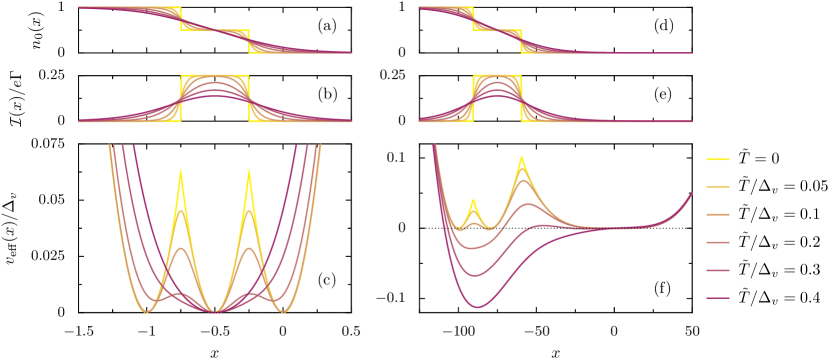
Figure 3: (Color online) For increasing temperature, (a,d) average occupation of the dot for fixed $x$, (b,e) quasistationary current and (c,f) effective potential, (a,b,c) far below the Euler instability ($\delta=-1$) and (d,e,f) at the instability ($\delta=0$). In the figure, $v=\Delta_{v}$, $v_{\mathrm{g}}=v_{\mathrm{g}}^{\mathrm{min}}$ and $\tilde{\alpha}=10^{-6}$.

At finite temperatures, the effective potential (15) qualitatively changes (see Fig. 3): the barriers separating the minima are lowered as one increases the temperature, leaving the effective potential with a single minimum for large enough temperatures. As detailed in Ref. weick11_PRB, , the current blockade becomes less pronounced as the temperature increases [see Fig. 8(a) below]. Moreover, taking into account the current-induced fluctuations (9) and dissipation (10) in the Langevin dynamics (5) further reduces the current blockade [see Fig. 11(a) below].

IV Current noise at the Euler buckling instability

We start by discussing the two contributions to the current noise, i.e., the usual shot noise and the mechanically-induced noise. It is the latter contribution to the noise which we find to be dramatically enhanced close to the mechanical instability.

The noise power spectrum is defined as blant00_PhysRep

$$S(\Omega)=2\int_{-\infty}^{+\infty}\mathrm{d}t\;\mathrm{e}^{\mathrm{i}\Omega t}\langle\Delta\hat{I}(t_{0}+t)\Delta\hat{I}(t_{0})\rangle,$$ (18)

where $\Delta\hat{I}(t)=\hat{I}(t)-\langle\hat{I}\rangle$ denotes the time-dependent fluctuations of the current operator. In Eq. (18), the brackets $\langle\ldots\rangle$ indicate an ensemble average or, equivalently, an average over the initial time $t_{0}$. Due to the separation of timescales between fast electronic dynamics and slow vibrational motion ($\omega\ll\Gamma$), one can identify two additive contributions to the noise power spectrum (18), $S=S_{\mathrm{sh}}+S_{\mathrm{m}}$. pisto08_PRB ; blant04_PRL ; mozyr06_PRB ; usman07_PRB The first one, $S_{\mathrm{sh}}$, corresponds to the (thermal) Nyquist-Johnson and shot noise and is discussed in Appendix A. The second contribution to Eq. (18), the mechanically-induced noise $S_{\mathrm{m}}$ (referred to as “mechanical noise” in the sequel), is induced by the fluctuations of the nanobeam deflection $x(t)$. These occur on a much longer timescale (of the order of $1/\omega$) than the shot noise (the corresponding current-current correlator decaying in that case on the short timescale $1/\Gamma$). The mechanically-induced noise therefore dominates the noise power spectrum at low frequencies, and can exceed the shot noise by orders of magnitude. pisto08_PRB ; blant04_PRL ; usman07_PRB ; mozyr06_PRB

The mechanical noise reads

$$S_{\mathrm{m}}(\Omega)= \;2\int\frac{\mathrm{d}\tau}{\omega_{0}}\;\mathrm{e}^{\mathrm{i}\Omega\tau/\omega_{0}}\int\mathrm{d}x\mathrm{d}p\mathrm{d}x_{0}\mathrm{d}p_{0}\;\Delta\mathcal{I}(x)$$

$$\times\mathcal{P}(x,p,\tau|x_{0},p_{0},\tau_{0})\Delta\mathcal{I}(x_{0})\mathcal{P}_{\mathrm{st}}(x_{0},p_{0})$$ (19)

where $\mathcal{P}(x,p,\tau|x_{0},p_{0},\tau_{0})$ is the conditional probability that the nanobeam is at phase-space point $(x,p)$ at time $\tau$, provided it was at $(x_{0},p_{0})$ at time $\tau_{0}\equiv 0$. In Eq. (IV), $\Delta\mathcal{I}(x)=\mathcal{I}(x)-I$ is the quasistationary current fluctuation, with $\mathcal{I}(x)$ and $I$ given by Eqs. (14) and (13), respectively. The conditional probability $\mathcal{P}(x,p,\tau|x_{0},p_{0},\tau_{0})$ can be obtained from the time-dependent solution of the Fokker-Planck equation (11) with the initial condition $\mathcal{P}(x,p,\tau_{0}|x_{0},p_{0},\tau_{0})=\delta(x-x_{0})\delta(p-p_{0})$. Equation (IV) can then be re-expressed by exploiting the above initial condition and performing the Laplace transform of the Fokker-Planck equation (11). This procedure yields pisto08_PRB

$$S_{\mathrm{m}}(\Omega)= -\frac{4}{\omega_{0}}\int\mathrm{d}x\mathrm{d}p\;\Delta\mathcal{I}(x)$$

$$\times\left[{\mathcal{L}}^{2}+\left(\frac{\Omega}{\omega_{0}}\right)^{2}\right]^{-1}{\mathcal{L}}\left[\Delta\mathcal{I}(x)\mathcal{P}_{\mathrm{st}}(x,p)\right],$$ (20)

with ${\mathcal{L}}$ the Fokker-Planck operator defined in Eq. (II). flind05_PhysicaE

In the form of Eq. (IV), the mechanical noise can be straightforwardly computed numerically, since it only requires the knowledge of the stationary probability distribution $\mathcal{P}_{\mathrm{st}}$ corresponding to the Fokker-Planck equation (11), as it is the case for the average current (13) (for details, see Ref. pisto08_PRB, ). footnote:numerics Alternatively, one can solve for the time-dependent solution $x(\tau)$ of the Langevin equation (5) using standard techniques for stochastic differential equations. kloeden The average current and noise are then computed by performing the time averages of the quasistationary current (14) and the current-current correlator entering Eq. (18), respectively. We have checked numerically that this approach yields the same results as the ones based on the stationary solution of the Fokker-Planck equation (11) [see Eqs. (13) and (IV)]. However, although more physically transparent, the method based on Eq. (5) requires long simulation times as well as sampling. We thus use the other method for all the numerical results presented in the sequel of the paper [except in Fig. 5, where we explicitly simulate the time-dependent deflection of the nanobeam from the Langevin equation (5)].

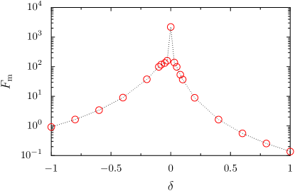
Figure 4: (Color online) Fano factor as a function of the reduced compression force $\delta$ [cf. Eq. (2)]. In the figure, $\gamma_{\mathrm{e}}=\omega_{0}/\Gamma=10^{-2}$, $\tilde{T}=3$, $\tilde{\alpha}=10^{-6}$, $v=\Delta_{v}$ and $v_{\mathrm{g}}=v_{\mathrm{g}}^{\mathrm{min}}$. The red circles correspond to the data points, while the dotted line serves as a guide to the eye.

In Fig. 4, we present our numerical results for the Fano factor $F_{\mathrm{m}}=S_{\mathrm{m}}(0)/2e|I|$, where the zero-frequency noise $S_{\mathrm{m}}(0)$ and the average current $I$, Eqs. (IV) and (13), respectively, are computed for typical parameters as a function of the reduced force $\delta$. In Fig. 4, the bias and gate voltages correspond to the apex of the Coulomb diamond [$v=\Delta_{v}$ and $v_{\mathrm{g}}=v_{\mathrm{g}}^{\mathrm{min}}$, cf. Eqs. (16) and (17), respectively]. As envisioned above, there is a dramatic increase of the mechanically-induced current noise in the vicinity of the Euler buckling instability ($\delta\approx 0$ in Fig. 4) as compared to the noise far away from the instability. Moreover, the Fano factor can take, depending on the compression force $\delta$, super-Poissonian values ($F_{\mathrm{m}}>1$) that are well above the shot noise contribution, $F_{\mathrm{sh}}=1/2$ (see Appendix A).

The results of Fig. 4 can essentially be understood in terms of telegraph noise in the effective potential (15) (see also Figs. 2 and 3). footnote:shuttle Indeed, unlike the energy gap (16) which varies algebraically with the force $\delta$ as $\sim 1/|\delta|$, the numerical results of Fig. 4 indicate that the noise (or Fano factor) depends exponentially on $1/|\delta|$ (notice the logarithmic scale in Fig. 4), suggesting telegraph noise. As the compression force increases towards the instability at $\delta=0$, the height of the barriers separating the three metastable minima (for $v=\Delta_{v}$) grows as the gap (16), such that the waiting time of the system in one of these minima increases exponentially. Thus, the probability for the system to switch to another minimum is drastically reduced, subsequently increasing the telegraph noise. As the height of the potential barriers near the Euler instability is very large, scaling as $1/\tilde{\alpha}^{1/3}$ with $\tilde{\alpha}\ll 1$ [see Fig. 2(f)], and the energy gap (16) is maximal at the instability, this leads to a current noise which is also maximal at the Euler instability.

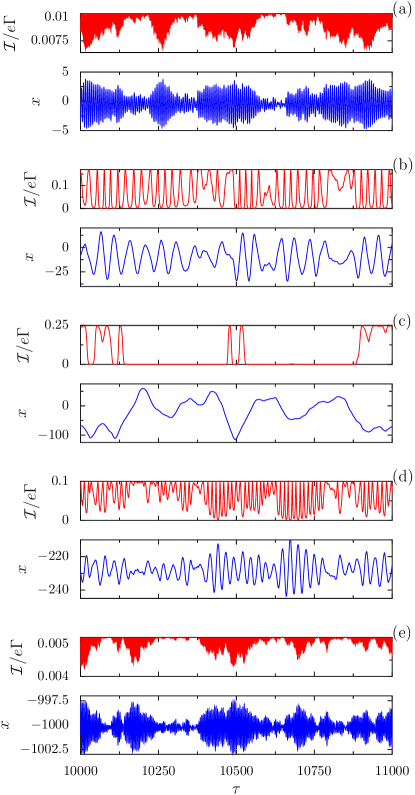
Figure 5: (Color online) Deflection $x$ (in blue) and quasistationary current $\mathcal{I}$ (in red) as a function of time simulated by the Langevin equation (5). In the figure, the compression force increases from (a) to (e): (a) $\delta=-1$, (b) $\delta=-0.05$, (c) $\delta=0$, (d) $\delta=0.05$, and (e) $\delta=1$. The parameters used in the figure are the same as in Fig. 4.

This interpretation is confirmed by Fig. 5, which shows the result of a simulation kloeden of the deflection of the nanobeam $x$ as a function of time (see blue lines in the figure) as obtained from the Langevin equation (5) for the same parameters as in Fig. 4. We also show the resulting quasistationary current (14) as a function of time by red lines in Fig. 5. Far from the instability [Figs. 5(a) and 5(e)], the dynamics of the nanobeam follows qualitatively the behavior of a Brownian particle in a harmonic potential. Indeed, for the temperature used in Figs. 4 and 5, the effective potential (15) far from the instability has a single minimum [see also Fig. 3(c)]. For temperatures $\tilde{T}$ which are large compared to the gap (16), the current shown in Figs. 5(a) and 5(e) switches rapidly between values which are small as compared to the maximal current $e\Gamma/4$ [cf. Fig. 3(b)]. Hence, the resulting Fano factor is relatively small (cf. Fig. 4). As one approaches the Euler instability from below [Fig. 5(b)] or above [Fig. 5(d)], the dynamics of the nanobeam becomes slower. Then the behavior of the current as a function of time starts to resemble telegraph noise, as the effective potential starts developing metastable minima for this value of the temperature as compared to the energy gap (16). At the instability [Fig. 5(c)], the dynamics of the nanobeam becomes very slow, and the behavior of the current as a function of time is completely stochastic and uncorrelated, with long waiting times between vanishing and maximal current. The corresponding Fano factor is thus extremely large and super-Poissonian ($F_{\mathrm{m}}>10^{3}$ in Fig. 4), and much larger than far from the Euler instability.

In order to understand the features of our main numerical results presented in Figs. 4 and 5 in more detail, we will first consider the role played by thermal fluctuations alone (Sec. V), while the full nonequilibrium dynamics is investigated further in Sec. VI.

V Thermal fluctuations

In this section, we consider the fully adiabatic limit $\omega_{0}/\Gamma\rightarrow 0$. We neglect the current-induced fluctuations and dissipation in the Fokker-Planck equation (11) [cf. Eqs. (9) and (10)] and consider the role played by thermal fluctuations alone. We start in Sec. V.1 with a simplified analytical model based on standard telegraph noise. In Sec. V.2 we substantiate our findings by evaluating Eq. (IV) numerically.

V.1 Telegraph noise

We present here an analytical estimate of the noise power spectrum. Our simplified model relies on thermally-induced telegraph noise machl54_JAP and on an estimate of the escape rates based on Kramers reaction rate theory. zwanzig ; krame40_Physica ; hangg90_RMP

In what follows, we work in the low-temperature regime $\tilde{T}\ll\Delta_{v}$, with the gap $\Delta_{v}$ given in Eq. (16). Moreover, we focus on the case where the nanobeam is far below the Euler instability ($-\delta\gg\tilde{\alpha}^{1/3}$), as the results presented below should stay qualitatively the same for larger compression forces. We thus approximate the effective potential (15) by its zero-temperature counterpart, which is shown in Fig. 2(c) for a gate voltage $v_{\mathrm{g}}=v_{\mathrm{g}}^{\mathrm{min}}$ [cf. Eq. (17)]. As one can see from Fig. 2(c), the effective potential has three metastable minima for $0<v<2\Delta_{v}$: two of them are equivalent (located symmetrically at $x_{1}=1/\delta$ and $x_{0}=0$ about the line $x=1/2\delta$) and correspond to a state in which the current vanishes [see Fig. 2(b)], while the one at $x_{1/2}=1/2\delta$ corresponds to a current-carrying state. This suggests to write a rate equation for the probabilities $P_{\mathrm{c}}$ and $P_{\mathrm{b}}$ that the system is in a conducting or blocked state, respectively. Denoting $\Gamma_{\mathrm{in}}=(\Gamma_{x_{0}\rightarrow x_{1/2}}+\Gamma_{x_{1}\rightarrow x_{1/2}})/2$ and $\Gamma_{\mathrm{out}}=\Gamma_{x_{1/2}\rightarrow x_{1}}+\Gamma_{x_{1/2}\rightarrow x_{0}}$ the transition rates in and out of the conducting state ($\Gamma_{x_{i}\rightarrow x_{j}}$ is here the transition rate from the minimum located at $x_{i}$ to the one at $x_{j}$), we have $\dot{P}_{\mathrm{c}}=-\dot{P}_{\mathrm{b}}=-\Gamma_{\mathrm{out}}P_{\mathrm{c}}+\Gamma_{\mathrm{in}}P_{\mathrm{b}}$. Following Ref. machl54_JAP, , the average current and the noise power spectrum are readily obtained from the above rate equation. They read

$$I=\frac{e\Gamma}{4}\frac{\Gamma_{\mathrm{in}}}{\Gamma_{\mathrm{in}}+\Gamma_{\mathrm{out}}}$$ (21)

and

$$S_{\mathrm{m}}(\Omega)=\frac{e^{2}\Gamma^{2}}{4}\frac{\Gamma_{\mathrm{in}}\Gamma_{\mathrm{out}}}{\Gamma_{\mathrm{in}}+\Gamma_{\mathrm{out}}}\frac{1}{\Omega^{2}+(\Gamma_{\mathrm{in}}+\Gamma_{\mathrm{out}})^{2}},$$ (22)

respectively. Notice that for bias voltages $v\geqslant 2\Delta_{v}$, the effective potential (15) has a single minimum [see Fig. 2(c)], and the telegraph noise model presented above does not apply. Instead, the system’s dynamics is characterized in that case by standard Brownian noise.

As detailed in Appendix B, the transition rates entering Eqs. (21) and (22) can be easily calculated using Kramers theory. krame40_Physica ; hangg90_RMP ; zwanzig Incorporating Eq. (30) in Eq. (21), we find for the average current the approximate expression

$$I=\frac{e\Gamma}{4}\left\{1+2\exp{\left[\frac{\Delta_{v}}{4\tilde{T}}\left(1-\frac{v}{\Delta_{v}}\right)\right]}\right\}^{-1},$$ (23)

valid for $v<2\Delta_{v}$. Using Eqs. (22) and (30), we find for the zero-frequency noise footnote:divergence

$$S_{\mathrm{m}}(0)= \,\frac{e^{2}\Gamma^{2}}{\omega_{0}}\gamma_{\mathrm{e}}^{-1}\frac{2\tilde{T}}{\Delta_{v}}h^{-1}\left(\frac{v}{2\Delta_{v}}\right)$$

$$\times\exp{\left(\frac{\Delta_{v}}{2\tilde{T}}\left[1-\frac{v}{\Delta_{v}}+\frac{1}{2}\left(\frac{v}{2\Delta_{v}}\right)^{2}\right]\right)}$$

$$\times\left\{1+2\exp{\left[\frac{\Delta_{v}}{4\tilde{T}}\left(1-\frac{v}{\Delta_{v}}\right)\right]}\right\}^{-3},$$ (24)

where the function $h(z)$ is defined in Eq. (31).

At a bias voltage corresponding to the energy gap (16) ($v=\Delta_{v}$), the results of Eqs. (23) and (V.1) simplify to yield the Fano factor

$$F_{\mathrm{m}}=\frac{16\Gamma}{3\omega_{0}}\gamma_{\mathrm{e}}^{-1}\frac{\tilde{T}}{\Delta_{v}}\exp{\left(\frac{\Delta_{v}}{16\tilde{T}}\right)}.$$ (25)

Although this result is based on a simplified model and despite the fact that it does not include the full nonequilibrium dynamics of the nanoresonator induced by the charge fluctuations on the dot, it qualitatively captures our main finding depicted in Fig. 4. Indeed, as one approaches the Euler instability from below, the gap $\Delta_{v}$ increases algebraically as $\sim 1/|\delta|$ [cf. Eq. (16)], resulting in an exponential increase of the Fano factor.

The results of Eqs. (23), (V.1) and (25) also apply for compression forces far above the Euler instability ($\delta\gg\tilde{\alpha}^{1/3}$). footnote:v_eff Since the energy gap $\Delta_{v}$ is, in that case, half of the gap far below the instability [$-\delta\gg\tilde{\alpha}^{1/3}$, cf. Eq. (16)], this explains the asymmetry of the Fano factor for negative and positive $\delta$ in Fig. 4. In the vicinity of the buckling instability ($|\delta|\ll\tilde{\alpha}^{1/3}$), the exponential dependence of the Fano factor as a function of the gap (16) (which here scales with $\tilde{\alpha}\ll 1$ as $1/\tilde{\alpha}^{1/3}$) should stay qualitatively the same. This results in a Fano factor which saturates at its maximal value at the Euler instability (cf. Fig. 4).

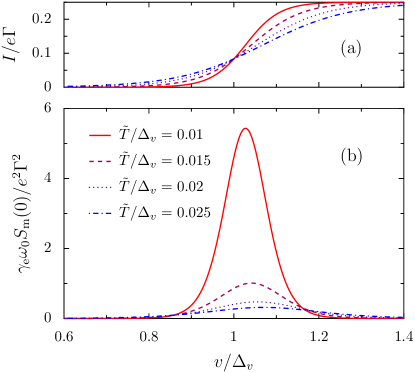
Figure 6: (Color online) (a) Current (23) and (b) zero-frequency noise (V.1) as a function of bias voltage for increasing temperature as obtained from the telegraph-noise model.

The results of Eqs. (23) and (V.1) for the average current and the zero-frequency noise are shown in Figs. 6(a) and 6(b), respectively. As one can see from Fig. 6(b), our analytical results capture the following trends for the mechanical noise: (i) it only depends on the compression force $\delta$ through the ratio $\tilde{T}/\Delta_{v}$, (ii) the noise is maximal close to $v=\Delta_{v}$ (a feature which has also been found in Ref. pisto08_PRB, in the case of fully coherent transport) and its maximum shifts towards higher bias voltages when one increases the temperature, and (iii) the noise is inversely proportional to the extrinsic damping constant (i.e., proportional to the quality factor). In Sec. V.2, these features based on our simplified telegraph-noise model will be confirmed and discussed further in the context of numerical calculations based on Eq. (IV).

V.2 Numerical results

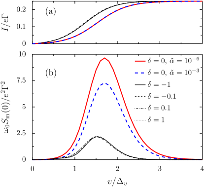
Figure 7: (Color online) (a) Current and (b) zero-frequency noise as a function of bias voltage for increasing values of the reduced compression force $\delta$. In the figure, $v_{\mathrm{g}}=v_{\mathrm{g}}^{\mathrm{min}}$, $\tilde{T}=\Delta_{v}/10$, $\gamma_{\mathrm{e}}=10^{-2}$, $\omega_{0}/\Gamma=0$ (no current-induced fluctuations), and $\tilde{\alpha}=10^{-6}$ for all lines except for the thick blue dashed one, where $\tilde{\alpha}=10^{-3}$.

In Fig. 7, we present numerical results for the average current [Fig. 7(a)] and the zero-frequency noise [Fig. 7(b)] as a function of bias voltage, for a gate voltage corresponding to the apex of the Coulomb diamond, see Eq. (17). As one can see from the figure, the noise has qualitatively the same behavior far from the Euler instability [$|\delta|\gg\tilde{\alpha}^{1/3}$, see thin black lines in Fig. 7(b)] and at the instability [$\delta=0$, thick lines in Fig. 7(b)]. Remarkably, the noise [as well as the current, see Fig. 7(a) and Ref. weick11_PRB, ], once plotted as a function of $v/\Delta_{v}$, and for the same value of $\tilde{T}/\Delta_{v}$, is (almost) quantitatively the same for any $\delta$ far from the instability [see thin black lines in Fig. 7(b)]. The overall behavior of the current and noise in Fig. 7 when the system is far from the Euler instability (see thin solid black lines in Fig. 7) can be understood in terms of the telegraph-noise model detailed previously. Indeed, Eq. (V.1) shows that for $\tilde{T}\ll\Delta_{v}$, the noise is exponentially sensitive to the ratio $\Delta_{v}/\tilde{T}$ only, thus explaining the scaling in Fig. 7(b). In contrast, the above scaling does not apply at the mechanical instability [see thick red and dashed blue lines in Fig. 7(b)]. There, the noise is larger for smaller values of the anharmonicity parameter $\tilde{\alpha}$, the latter determining the strength of the quartic correction in the effective potential (15).

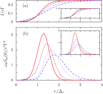
Figure 8: (Color online) (a) Current and (b) zero-frequency noise as a function of bias voltage for increasing temperature $\tilde{T}=0.03$ (solid line), $0.04$ (dashed line), $0.06$ (dotted line), $0.08$ (dash-dotted line). In the figure, $\delta=-1$, $v_{\mathrm{g}}=v_{\mathrm{g}}^{\mathrm{min}}$, $\gamma_{\mathrm{e}}=10^{-2}$, $\omega_{0}/\Gamma=0$, and $\tilde{\alpha}=10^{-6}$. Insets: Same as the main figure for $\delta=0$. In the insets, $\tilde{T}=2$ (solid line), $2.5$ (dashed line), $3$ (dotted line), $3.5$ (dash-dotted line).

In Fig. 8, we present the temperature dependence of both the current and the zero-frequency noise far below the Euler instability [Figs. 8(a) and 8(b), respectively] and at the instability (see insets in Fig. 8). As one can see from the figure, the behavior of these two quantities is qualitatively the same far from and at the buckling instability. As temperature increases, the current blockade becomes less pronounced [see Fig. 8(a)] as the system can explore more phase-space due to thermal fluctuations (for more details, see Ref. weick11_PRB, ). Moreover, the maximum of the zero-frequency noise decreases with temperature and gets shifted to larger values of the bias voltage [see Fig. 8(b)], a phenomenon which is captured by our analytical estimate of the noise in Sec. V.1 (see Fig. 6). As temperature increases, the probability to jump out of one minimum of the effective potential (cf. Fig. 2) increases exponentially, such that the associated telegraph noise decreases.

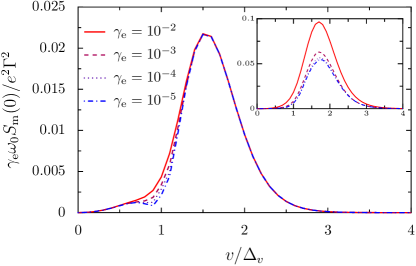
Figure 9: (Color online) Zero-frequency noise as a function of bias voltage for increasing values of the extrinsic damping constant (or inverse quality factor) $\gamma_{\mathrm{e}}$. In the figure, $\delta=-1$, $v_{\mathrm{g}}=v_{\mathrm{g}}^{\mathrm{min}}$, $\tilde{T}=\Delta_{v}/10$, $\omega_{0}/\Gamma=0$, and $\tilde{\alpha}=10^{-6}$. Inset: Same as the main figure for $\delta=0$.

In Fig. 9, we show numerical results for the zero-frequency noise for various values of the extrinsic damping constant $\gamma_{\mathrm{e}}=1/Q$ (or inverse quality factor) far below the instability (Fig. 9) and at the Euler instability (inset in Fig. 9). As one can see from the main figure, the mechanically-induced noise scales almost perfectly as $S_{\mathrm{m}}(0)\sim\gamma_{\mathrm{e}}^{-1}$ for compression forces far below the instability. This is characteristic of telegraph noise in the weak friction limit, krame40_Physica ; hangg90_RMP where the system’s energy varies only slowly with time [cf. Appendix B and Eq. (V.1)]. Interestingly, in the case of molecular devices, the noise is also much larger for unequilibrated (high-$Q$) vibrons. koch05_PRL ; koch06_PRB At the instability (see the inset in Fig. 9), the scaling with $\gamma_{\mathrm{e}}$ is only approximate. footnote:gamma_e

We conclude this section by computing the frequency dependence of the mechanical noise (IV) far below (Fig. 10) and at the Euler instability (inset in Fig. 10). Far from the instability, the frequency dependence of the noise shows a $1/f^{2}$ dependence, typical of telegraph noise [cf. Eq. (22)]. Notice that the width of the Lorentzian shape of $S_{\mathrm{m}}(\Omega)$ depends on the bias voltage through the transition rates for the system to enter or leave the conducting minimum corresponding to an average occupation of the dot of $1/2$, see Eqs. (22) and (30). At the Euler buckling instability, $S_{\mathrm{m}}(\Omega)$ also follows a $1/f^{2}$ behavior for $\Omega\ll\omega_{0}$, although additional structures appear for larger frequencies and for certain bias voltages. footnote:frequency

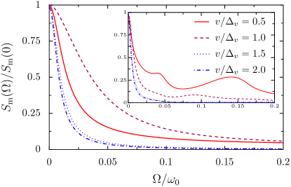
Figure 10: (Color online) Frequency dependence of the mechanical noise for various values of the bias voltage. In the figure, $\delta=-1$, $v_{\mathrm{g}}=v_{\mathrm{g}}^{\mathrm{min}}$, $\tilde{T}=\Delta_{v}/10$, $\tilde{\alpha}=10^{-6}$, $\gamma_{\mathrm{e}}=10^{-2}$, and $\omega_{0}/\Gamma=0$. (Inset) Same as the main figure for $\delta=0$.

VI Nonequilibrium fluctuations

We now investigate the mechanical noise in the presence of the current-induced fluctuations and dissipation, Eqs. (9) and (10).

Our numerical results for the current and the zero-frequency noise are shown in Figs. 11(a) and 11(b), respectively, when the nanobeam is at the Euler instability (the insets in Fig. 11 consider the case $\delta=-1$). As one can see from Fig. 11, the effect of an increasing adiabaticity parameter $\omega_{0}/\Gamma$, which controls the strength of the current-induced fluctuations (9) and dissipation (10), is qualitatively similar to the effect of an increasing temperature (cf. Fig. 8). Indeed, the overall noise level is reduced and the maximum of the noise is shifted towards larger bias voltages for increasing $\omega_{0}/\Gamma$ [see Fig. 11(b)]. Moreover, the current blockade gets less pronounced for increasing $\omega_{0}/\Gamma$ [see Fig. 11(a)].

The results of Fig. 11 can be qualitatively understood by defining an effective temperature weick11_PRB ; weick11b_PRB

$$\tilde{T}_{\mathrm{eff}}=\frac{\langle d\rangle/2+\gamma_{\mathrm{e}}\tilde{T}}{\langle\gamma\rangle+\gamma_{\mathrm{e}}}$$ (26)

in analogy with the fluctuation-dissipation theorem. zwanzig Here, $\langle d\rangle$ and $\langle\gamma\rangle$ are the averages over phase-space of the current-induced fluctuations and dissipation, Eqs. (9) and (10), respectively. As shown in Ref. weick11_PRB, , the effective temperature (26) is approximately given by $\tilde{T}_{\mathrm{eff}}\simeq\tilde{T}+\frac{\omega_{0}/\Gamma}{4\gamma_{\mathrm{e}}}\Theta(v-\Delta_{v})$, with $\Theta(z)$ the Heaviside step function. This explains why both the current and the zero-frequency noise are quite insensitive to the ratio $\omega_{0}/\Gamma$ for $v<\Delta_{v}$ and are similar to the case $\omega_{0}/\Gamma=0$, i.e., the fully adiabatic limit. On the contrary, for $v>\Delta_{v}$, the effective temperature increases with increasing $\omega_{0}/\Gamma$, explaining the similarity of the behavior of the current and noise in Figs. 11 and 8.

We conclude this section by noticing that we have numerically checked that the frequency dependence of the noise power spectrum also follows a $1/f^{2}$ behavior when one takes into account current-induced fluctuations, similar to Fig. 10. This confirms that the noise is dominated by a telegraph noise at low-enough temperatures even in presence of nonequilibrium fluctuations.

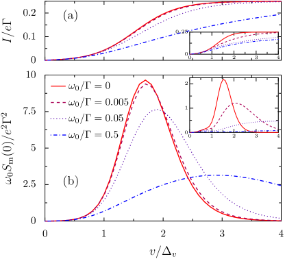
Figure 11: (Color online) (a) Current and (b) zero-frequency noise as a function of bias voltage for increasing values of the adiabaticity parameter $\omega_{0}/\Gamma$. In the figure, $\delta=0$, $v_{\mathrm{g}}=v_{\mathrm{g}}^{\mathrm{min}}$, $\gamma_{\mathrm{e}}=10^{-2}$, $\tilde{T}/\Delta_{v}=0.1$ and $\tilde{\alpha}=10^{-6}$. (Inset) Same as the main figure with $\delta=-1$.

VII Conclusion

We have investigated the current noise in nanoelectromechanical systems close to a continuous mechanical instability. Specifically, we have considered the paradigmatic Euler buckling instability in suspended single-electron transistors which are capacitively coupled to a gate electrode. We have predicted a drastic enhancement of the current noise when the nanobeam supporting the quantum dot is brought to the Euler instability, resulting in very large Fano factors that are well above the Poisson limit. This exponential enhancement at the buckling instability is directly related to the (algebraic) enhancement of the current blockade predicted in Ref. weick11_PRB, . We developed a rather detailed picture of the underlying physics in terms of a telegraph-noise model. While such large Fano factors may make observation of the low-bias current blockade more challenging, the large noise levels predicted in this work would serve also as a clear experimental signature of the interplay between electronic and mechanical degrees of freedom in NEMS (e.g., carbon nanotubes onac06_PRL ) close to continuous mechanical instabilities.

Appendix A Shot noise

In this appendix, we briefly comment on how the shot noise properties of the setup considered in this paper (see Fig. 1) are influenced by the coupling (4) between the charge on the quantum dot and the mechanical degree of freedom.

Within the adiabatic approach presented in Sec. II, the shot noise reads

$$S_{\mathrm{sh}}(\Omega)=\int\mathrm{d}x\mathrm{d}p\;\mathcal{P}_{\mathrm{st}}(x,p)\mathcal{S}_{\mathrm{sh}}(\Omega,x),$$ (27)

where $\mathcal{S}_{\mathrm{sh}}(\Omega,x)$ is the quasistationary shot noise for fixed position $x$. Its zero-frequency limit ($\Omega\ll\Gamma$) blant00_PhysRep reads in the sequential-tunneling regime ($\hbar\Gamma\ll k_{\mathrm{B}}T$)

$$\mathcal{S}_{\mathrm{sh}}(0,x)=\frac{e^{2}\Gamma}{4}\left[f_{\mathrm{L}}(x)+f_{\mathrm{R}}(x)\right]\left[2-f_{\mathrm{L}}(x)-f_{\mathrm{R}}(x)\right]$$ (28)

where $f_{\mathrm{L/R}}(x)$ are the Fermi factors defined in Eq. (8).

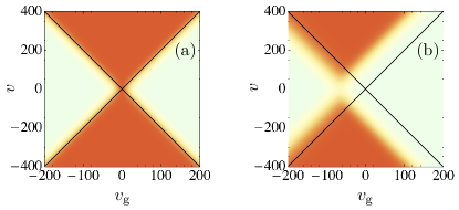
Figure 12: (Color online) Zero-frequency shot noise as a function of bias $v$ and gate voltage $v_{\mathrm{g}}$ (a) for vanishing compression force $F=0$ and (b) at the Euler buckling instability where $F=F_{\mathrm{c}}$. The parameters used in the figure are $\tilde{T}=10$, $\tilde{\alpha}=10^{-6}$, $\omega_{0}/\Gamma=10^{-2}$, and $\gamma_{\mathrm{e}}=1/Q=10^{-2}$. Color scale: white and red (light gray) regions correspond to $S_{\mathrm{sh}}(0)=0$ and $e^{2}\Gamma/4$, respectively.

In the strictly adiabatic limit $\omega_{0}/\Gamma\rightarrow 0$, the current-induced fluctuation and damping coefficients are both vanishing [see Eqs. (9) and (10)], such that the stationary probability distribution function corresponding to the Fokker-Planck equation (11) is a Boltzmann distribution at temperature $\tilde{T}$. Assuming zero temperature, the (zero-frequency) shot noise (27) reduces to $S_{\mathrm{sh}}(0)=\mathcal{S}_{\mathrm{sh}}(0,x_{\mathrm{m}})$, with $x_{\mathrm{m}}$ the global minimum of the effective potential (15). weick11_PRB Thus, the shot noise observes the same behavior as the mean-field current discussed in Ref. weick11_PRB, : In the $v$-$v_{\mathrm{g}}$ plane, the shot noise has the same structure as the Coulomb diamonds delimited by slopes $v\sim\pm 2v_{\mathrm{g}}$, the apex of these diamonds being given by Eqs. (16) and (17). The zero-frequency shot noise thus takes the value $S_{\mathrm{sh}}(0)=e^{2}\Gamma/4=e|I|$ in the conducting regions of the $v$-$v_{\mathrm{g}}$ plane, with a corresponding Fano factor $F_{\mathrm{sh}}=S_{\mathrm{sh}}(0)/2e|I|$ of $1/2$, typical for a single-level quantum dot symmetrically coupled to source and drain leads in the sequential-tunneling regime. blant00_PhysRep The behavior of the mean-field zero-frequency shot noise as a function of the reduced compression force $\delta$ can thus readily be deduced from the behavior of the mean-field current shown in Fig. 4 of Ref. weick11_PRB, (see also Fig. 2 in Ref. weick11b_PRB, ).

Including thermal as well as current-induced fluctuations by solving for the stationary solution of the Fokker-Planck equation (11) numerically and computing the shot noise with the help of Eq. (27) leads to qualitatively the same effects as for the average current. This is exemplified in Fig. 12, where fluctuations lead to a softening of the borders in the $v$-$v_{\mathrm{g}}$ plane delimiting the regions with a finite shot noise $S_{\mathrm{sh}}\simeq e^{2}\Gamma/4$.

Appendix B Transition rates

The transition rates $\Gamma_{\mathrm{in}}$ and $\Gamma_{\mathrm{out}}$ entering our approximate expressions for the average current (21) and the noise power spectrum (22) can be calculated using Kramers reaction rate theory. krame40_Physica ; hangg90_RMP ; zwanzig In the weak damping regime, which is the experimentally relevant one for carbon nanotube-based resonators that can present very high quality factors, steel09_Science ; lassa09_Science the escape rate from the minimum located at $x_{i}$ is given by

$$k_{x_{i}}=\gamma_{\mathrm{e}}\frac{\omega_{0}\sqrt{v_{\mathrm{eff}}^{\prime\prime}(x_{i})}}{2\pi\tilde{T}}S_{0}(v_{\mathrm{b},i})\exp{\left(-\frac{v_{\mathrm{b},i}}{\tilde{T}}\right)},$$ (29)

where $S_{0}(v_{\mathrm{b},i})$ is the abbreviated action at the barrier top, whose energy, seen from $x_{i}$, is denoted by $v_{\mathrm{b},i}$. Notice that Eq. (29) is valid as long as $\tilde{T}\ll v_{\mathrm{b},i}$ and in the weak damping regime, i.e., $\gamma_{\mathrm{e}}S_{0}(v_{\mathrm{b},i})\ll\tilde{T}$. hangg90_RMP With Eq. (29), and taking into account the probability that the system thermalizes in the well it jumps to, hangg90_RMP we find for the transition rates

$$\Gamma_{\mathrm{in}} =\gamma_{\mathrm{e}}\omega_{0}\frac{\Delta_{v}}{4\tilde{T}}h\left(\frac{v}{2\Delta_{v}}\right)\exp{\left(-\frac{\Delta_{v}}{4\tilde{T}}\left[1-\frac{v}{2\Delta_{v}}\right]^{2}\right)},$$ (30a)

$$\Gamma_{\mathrm{out}} =\gamma_{\mathrm{e}}\omega_{0}\frac{\Delta_{v}}{2\tilde{T}}h\left(\frac{v}{2\Delta_{v}}\right)\exp{\left(-\frac{\Delta_{v}}{4\tilde{T}}\left[\frac{v}{2\Delta_{v}}\right]^{2}\right)},$$ (30b)

with

$$h(z)=\frac{z^{2}(1-z)^{2}}{z^{2}+2(1-z)^{2}}.$$ (31)

References

- (1) H. G. Craighead, Science 290, 1532 (2000).
- (2) K. L. Ekinci and M. L. Roukes, Rev. Sci. Instrum. 76, 061101 (2005).
- (3) M. Poot and H. S. J. van der Zant, Phys. Rep. 511, 273 (2012).
- (4) F. Pistolesi and S. Labarthe, Phys. Rev. B 76, 165317 (2007).
- (5) F. Pistolesi, Y. M. Blanter, and I. Martin, Phys. Rev. B 78, 085127 (2008).
- (6) J. Koch and F. von Oppen, Phys. Rev. Lett. 94, 206804 (2005).
- (7) J. Koch, F. von Oppen, and A. V. Andreev, Phys. Rev. B 74, 205438 (2006).
- (8) R. Leturcq, C. Stampfer, K. Inderbitzin, L. Durrer, C. Hierold, E. Mariani, M. G. Schultz, F. von Oppen, and K. Ensslin, Nature Phys. 5, 327 (2009).
- (9) G. A. Steele, A. K. Hüttel, B. Witkamp, M. Poot, H. B. Meerwaldt, L. P. Kouwenhoven, and H. S. J. van der Zant, Science 325, 1103 (2009).
- (10) B. Lassagne, Y. Tarakanov, J. Kinaret, D. Garcia-Sanchez, and A. Bachtold, Science 325, 1107 (2009).
- (11) G. Weick, F. von Oppen, and F. Pistolesi, Phys. Rev. B 83, 035420 (2011).
- (12) G. Weick and D. M.-A. Meyer, Phys. Rev. B 84, 125454 (2011).
- (13) L. D. Landau and E. M. Lifshitz, Theory of Elasticity (Pergamon, Oxford, 1970).
- (14) T. Novotný, A. Donarini, C. Flindt, and A.-P. Jauho, Phys. Rev. Lett. 92, 248302 (2004).
- (15) F. Pistolesi, Phys. Rev. B 69, 245409 (2004).
- (16) Y. M. Blanter, O. Usmani, and Y. V. Nazarov, Phys. Rev. Lett. 93, 136802 (2004); 94, 049904(E) (2005).
- (17) A. D. Armour, Phys. Rev. B 70, 165315 (2004).
- (18) C. Flindt, T. Novotný, and A.-P. Jauho, Europhys. Lett. 69, 475 (2005).
- (19) A. Donarini, T. Novotný, and A.-P. Jauho, New. J. Phys. 7, 237 (2005).
- (20) O. Usmani, Y. M. Blanter, and Y. V. Nazarov, Phys. Rev. B 75, 195312 (2007).
- (21) D. Mozyrsky, M. B. Hastings, and I. Martin, Phys. Rev. B 73, 035104 (2006).
- (22) R. Hussein, A. Metelmann, P. Zedler, and T. Brandes, Phys. Rev. B 82, 165406 (2010).
- (23) A. Nocera, C. A. Perroni, V. Marigliano Ramaglia, and V. Cataudella, Phys. Rev. B 83, 115420 (2011).
- (24) N. Bode, S. Viola Kusminskiy, R. Egger, and F. von Oppen, Phys. Rev. Lett. 107, 036804 (2011).
- (25) N. Bode, S. Viola Kusminskiy, R. Egger, and F. von Oppen, Beilstein J. Nanotechnol. 3, 144 (2012).
- (26) G. Weick, F. Pistolesi, E. Mariani, and F. von Oppen, Phys. Rev. B 81, 121409(R) (2010).
- (27) S. M. Carr, W. E. Lawrence, and M. N. Wybourne, Phys. Rev. B 64, 220101(R) (2001).
- (28) P. Werner and W. Zwerger, Europhys. Lett. 65, 158 (2004).
- (29) V. Peano and M. Thorwart, New J. Phys. 8, 21 (2006).
- (30) S. Savel’ev, X. Hu, and F. Nori, New J. Phys. 8, 105 (2006).
- (31) S. Sapmaz, Y. M. Blanter, L. Gurevich, and H. S. J. van der Zant, Phys. Rev. B 67, 235414 (2003).
- (32) R. Zwanzig, Nonequilibrium Statistical Mechanics (Oxford University Press, Oxford, 2001).
- (33) Far above the Euler instability (), the effective potential has, close to , approximately the same form as for , cf. Fig. 2(c).
- (34) Y. M. Blanter and M. Büttiker, Phys. Rep. 336, 1 (2000).
- (35) For a derivation of Eq. (IV), see also C. Flindt, T. Novotný, and A.-P. Jauho, Physica E 29, 411 (2005).
- (36) The stationary solution of the Fokker-Planck equation (11) is obtained by discretizing phase-space over a finite grid using vanishing boundary conditions and taking advantage of the normalization condition .
- (37) P. Kloeden and E. Platen, Numerical Solution of Stochastic Differential Equations (Springer, Berlin, 1999).
- (38) Note that, in the somewhat different context of the quantum shuttle, large Fano factors have been predicted in Refs. flind05_EPL, and donar05_NJP, in the so-called “coexistence regime”, which were interpreted in terms of telegraph noise.
- (39) S. Machlup, J. Appl. Phys. 25, 341 (1954).
- (40) H. A. Kramers, Physica 7, 284 (1940).
- (41) P. Hänggi, P. Talkner, and M. Borkovec, Rev. Mod. Phys. 62, 251 (1990).
- (42) The apparent divergence of this result for and is unphysical as these bias voltages are out of the range of validity of the transition rates (30) entering Eq. (22) (cf. the weak friction limit).
- (43) As we have checked, for the largest values of used in the inset in Fig. 9, the weak-friction limit used in Appendix B of Kramers reaction rate theory is no longer strictly valid, such that the scaling is only approximate.
- (44) These features cannot be explained by our telegraph-noise model presented above. This might be due, e.g., to the asymmetry of the effective potential at [see Fig. 2(f)] which is not incorporated in our analytical model, the latter being in principle only valid far below the instability.
- (45) E. Onac, F. Balestro, B. Trauzettel, C. F. J. Lodewijk, and L. P. Kouwenhoven, Phys. Rev. Lett. 96, 026803 (2006).