Nanoflare Evidence from Analysis of the X-Ray Variability of an Active Region Observed with Hinode/XRT

Abstract

The heating of the solar corona is one of the big questions in astrophysics. Rapid pulses called nanoflares are among the best candidate mechanisms. The analysis of the time variability of coronal X-ray emission is potentially a very useful tool to detect impulsive events. We analyze the small-scale variability of a solar active region in a high cadence Hinode/XRT observation. The dataset allows us to detect very small deviations of emission fluctuations from the distribution expected for a constant rate. We discuss the deviations in the light of the pulsed-heating scenario.

¹Dipartimento di Scienze Fisiche ed Astronomiche, Università degli studi di Palermo, Via Archirafi 36, 90123, Palermo, Italy

²INAF Osservatorio Astronomico di Palermo, Piazza del Parlamento 1, 90134 Palermo, Italy

³National Astronomical Observatory of Japan, 2-21-1 Osawa, Mitaka, Tokyo, 181-8588, Japan

⁴NASA Goddard Space Flight Center, Greenbelt, MD 20771, USA

1 Introduction

The investigation of the heating mechanisms of the confined coronal plasma is still under intense debate. It is widely believed that the energy source for coronal heating is the magnetic energy stored in the solar corona. An unsolved problem is how this magnetic energy is converted into thermal energy of the confined coronal plasma. As Parker proposed in 1988, rapid pulses called nanoflares are among the best candidate mechanisms of magnetic energy release. Nowadays a challenging problem is to obtain evidence that such nanoflares are really at work. If small energy discharges (nanoflares) contribute in some way to coronal heating, they could be too small and frequent to be resolved as independent events. In this case, we would need to search for indirect evidence.

The idea of this work is that, if the solar corona emission is sustained by repeated nanoflares, locally the X-ray emission may not be entirely constant but may show variations around the mean intensity. So nanoflares may leave their signature on the light curves. Many authors (Shimizu & Tsuneta 1997; Vekstein & Katsukawa 2000; Katsukawa & Tsuneta 2001; Katsukawa 2003; Sakamoto et al. 2008) pointed out that a detailed analysis of intensity fluctuations of the coronal X-ray emission could give us information on these smallest flares. Following this hint we use this approach for the first time on Hinode data, searching, with statistical analysis, for small but systematic variability in noisy background light curves and their link to coronal heating models.

2 Instruments and Data

The Japanese Hinode satellite was launched in 2006 (Kosugi et al. 2007). One of the instruments it carries is the X-Ray Telescope (XRT), a high resolution grazing incidence telescope (Golub et al. 2007; Kano et al. 2008) that images the Sun through nine X-ray filters, using two filter wheels.

In our work we analyze the active region (AR) 10923, observed when it was located close to the disk center on November 14, 2006. The data set consists of $303$ images of $256\times 256$ pixels, taken in the Al_poly filter with an average cadence of about 6 s, for a total coverage of the observation of about $26$ minutes.

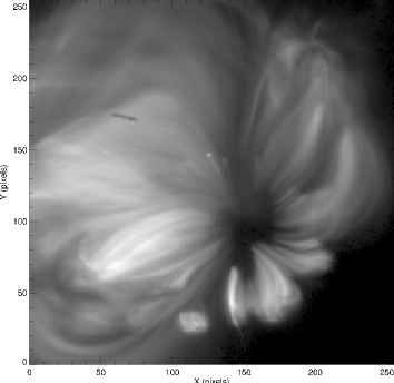
Figure 1.: Left: Average intensity map of the analyzed field of view ($256\times 256$ pixels), taken by Hinode/XRT on November 14, 2006, through the Al_poly filter. Right: Example of pixel light curve. The $y$-axis shows intensity in DN s^-1, the $x$-axis is time in s.

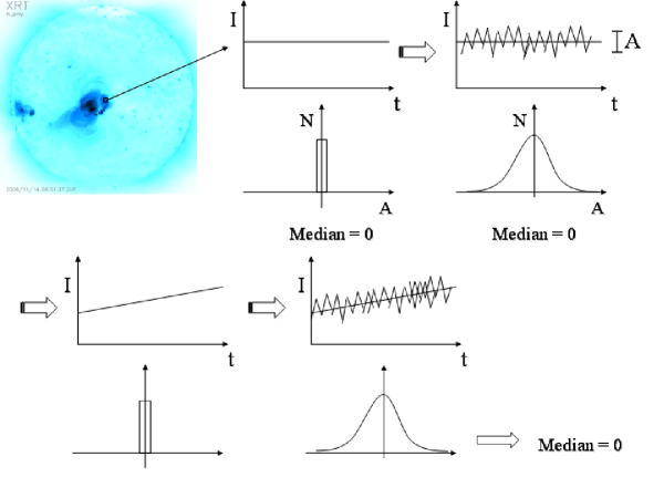
Figure 2.: Schematic concept of this work. Consider the light curve of a valid pixel. If the count rate is constant, the histogram of fluctuations is trivial. If we add the expected photon noise and the count rate is high we expect a broad Gaussian distribution of the fluctuations. We expect the same distribution if the count rate is linearly changing.

3 Data Analysis

In this work we analyze the intensity fluctuations of a high cadence XRT observation, searching for signal on top of statistical fluctuations, and its link to coronal heating model. Figure 2 is a flow chart which describes the concept of our analysis. Let us consider the light curve of a pixel in the AR and let us build the histogram of the amplitude of the fluctuations with respect to the average emission trend. If the count rate is strictly constant, the histogram of fluctuations is trivial. However, fluctuations are intrinsic to the finite photon counting. If we add the expected photon noise and the count rate is high, we expect an almost Gaussian distribution of the fluctuations, symmetric around zero, i.e., we expect an equal amount of positive and negative fluctuations. We expect the same distribution if the count rate is linearly and moderately changing instead of being constant. Even for a large curve with a constant rate we expect a broad distribution of fluctuations due to photon noise. If the count rate is high the distribution is approximately Gaussian. We expect exactly the same distributions also if the count rate is linearly changing instead of being constant, as sketched in Figure 2.

Along this line, for each pixel we create the distribution of intensity fluctuations of the light curve. We normalize the amplitude of the fluctuations to the photon noise $\sigma_{\rm p}$, expected from determining the original photons impacting on the detector from the measured readout. The conversion from DN to photon counts is through the conversion factor $K^{(2)}_{i}$ for the $i$-th filter-band:

$$\sigma_{\rm p}=\sqrt{K^{(2)}_{i}(T)I_{0}},$$ (1)

where $T$ is the electron temperature and $I_{0}$ is the measured DN.

The conversion factor is obtained as:

$$K^{(2)}_{i}=\frac{\int{[(hc/\lambda)/(57\times 3.65{\rm eV})]\,P(\lambda,T)\,\eta_{i}(\lambda)\,{\rm d}\lambda}}{\int{P(\lambda,T)\,\eta_{i}(\lambda)\,{\rm d}\lambda}},$$ (2)

where $P(\lambda,T)$ is the emissivity as a function of wavelength $\lambda$ and electron temperature $T$, and $\eta_{i}(\lambda)$ is the telescope effective area. For the moment, we assume a temperature $\log T=6.3$ (Kano & Tsuneta 1995; Narukage et al. 2011).

Figure 3.: Top: Distribution of the fluctuations of a pixel light curve, with respect to the linear fit to the light curve (solid line) in comparison with a symmetric Gaussian-like distribution (dashed line). Bottom: Residuals of the fluctuations with respect to the Gaussian curve.

Since we are interested in low amplitude systematic variations, we first remove pixels with low signals and those showing all kinds of high or slow amplitude systematic variations, such as:

• Pixels with spikes due to cosmic rays

• Pixels that show micro-flares or other transient brightenings

• Pixels that show slow variations due, for instance, to local loop drift or loop motion.

At the end of this data screening we are left with about $56\%$ of total pixels. The light curves of all these pixels can be fit with linear regression. An an example of our analysis, in Fig. 3 we show the result for one pixel (1,1).

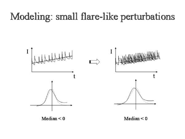
Figure 4.: Schematic concept of expectations from light curves perturbed by trains of small flare-like events. Although the mean emission would not change, the distribution of the fluctuations would become asymmetric, with a negative median even in the presence of significant photon noise.

3.1 Results

For each pixel we build the histogram of the X-ray intensity fluctuations with respect to the linear fit line. Figure 3 shows a sample distribution for one pixel compared to a symmetric Gaussian distribution. By inspecting the figure, we realize that there is a slight excess of the number of negative fluctuations over the number of positive ones. This excess makes the histogram slightly asymmetric toward the left side of the distribution. The excess is present but not very significant on most of the single pixel signal over the noise (as we can see in Figure 3).

From preliminary analysis, the excess becomes more significant when we apply the analysis to selected subregions localized in different part of the active region and even more when we sum over the whole region.

4 Conclusions

In summary, histograms of light curve fluctuations measured at high cadence show asymmetric distributions with median lower than zero. Asymmetries seem to appear at all scales from single pixels, sub-regions, to the whole active region at high confidence level. We propose that the asymmetry of the distributions of the fluctuations could be compatible with random sequences of small fast rise and slow decay pulses. This is typical of flare-like evolution (Reale 2010). Figure 4 sketches the concept of this scenario: the presence of trains of small flare-like events would make the distributions of fluctuations asymmetric in the observed direction. The median would be negative because the light curve will spend more time below than above the average trend, i.e., the mean for a constant light curve. Preliminary modeling using Monte Carlo simulations appears to support this scenario. In our opinion, if confirmed, these results would support a widespread storm-of-nanoflares scenario. We emphasize that this analysis requires high-cadence XRT observations. Improved diagnostics would be obtained if at least a few images were available in different filter bands.

Acknowledgments

Hinode is a Japanese mission developed and launched by ISAS/JAXA, with NAOJ as domestic partner and NASA and STFC (UK) as international partners. It is operated by these agencies in cooperation with ESA and NSC (Norway). ST, FR, and MM acknowledge support from Italian Ministero dell’Università e Ricerca and Agenzia Spaziale Italiana (ASI), contract I/023/09/0.

References

- Golub et al. (2007) Golub, L., Deluca, E., Austin, G., Bookbinder, J., Caldwell, D., Cheimets, P., Cirtain, J., Cosmo, M., Reid, P., Sette, A., Weber, M., Sakao, T., Kano, R., Shibasaki, K., Hara, H., Tsuneta, S., Kumagai, K., Tamura, T., Shimojo, M., McCracken, J., Carpenter, J., Haight, H., Siler, R., Wright, E., Tucker, J., Rutledge, H., Barbera, M., Peres, G., & Varisco, S. 2007, Solar Phys., 243, 63
- Kano et al. (2008) Kano, R., Sakao, T., Hara, H., Tsuneta, S., Matsuzaki, K., Kumagai, K., Shimojo, M., Minesugi, K., Shibasaki, K., Deluca, E. E., Golub, L., Bookbinder, J., Caldwell, D., Cheimets, P., Cirtain, J., Dennis, E., Kent, T., & Weber, M. 2008, Solar Phys., 249, 263
- Kano & Tsuneta (1995) Kano, R., & Tsuneta, S. 1995, ApJ, 454, 934
- Katsukawa (2003) Katsukawa, Y. 2003, PASJ, 55, 1025
- Katsukawa & Tsuneta (2001) Katsukawa, Y., & Tsuneta, S. 2001, ApJ, 557, 343
- Kosugi et al. (2007) Kosugi, T., Matsuzaki, K., Sakao, T., Shimizu, T., Sone, Y., Tachikawa, S., Hashimoto, T., Minesugi, K., Ohnishi, A., Yamada, T., Tsuneta, S., Hara, H., Ichimoto, K., Suematsu, Y., Shimojo, M., Watanabe, T., Shimada, S., Davis, J. M., Hill, L. D., Owens, J. K., Title, A. M., Culhane, J. L., Harra, L. K., Doschek, G. A., & Golub, L. 2007, Solar Phys., 243, 3
- Narukage et al. (2011) Narukage, N., Sakao, T., Kano, R., Hara, H., Shimojo, M., Bando, T., Urayama, F., Deluca, E., Golub, L., Weber, M., Grigis, P., Cirtain, J., & Tsuneta, S. 2011, Solar Phys., 269, 169
- Parker (1988) Parker, E. N. 1988, ApJ, 330, 474
- Reale (2010) Reale, F. 2010, Living Reviews in Solar Physics, 7, 5
- Sakamoto et al. (2008) Sakamoto, Y., Tsuneta, S., & Vekstein, G. 2008, ApJ, 689, 1421
- Shimizu & Tsuneta (1997) Shimizu, T., & Tsuneta, S. 1997, ApJ, 486, 1045
- Vekstein & Katsukawa (2000) Vekstein, G., & Katsukawa, Y. 2000, ApJ, 541, 1096