The Melnikov method and subharmonic orbits in a piecewise smooth system

Abstract

In this work we consider a two-dimensional piecewise smooth system, defined in two domains separated by the switching manifold $x=0$. We assume that there exists a piecewise-defined continuous Hamiltonian that is a first integral of the system. We also suppose that the system possesses an invisible fold-fold at the origin and two heteroclinic orbits connecting two hyperbolic critical points on either side of $x=0$. Finally, we assume that the region closed by these heteroclinic connections is fully covered by periodic orbits surrounding the origin, whose periods monotonically increase as they approach the heteroclinic connection.
When considering a non-autonomous ($T$-periodic) Hamiltonian perturbation of amplitude $\varepsilon$, using an impact map, we rigorously prove that, for every $n$ and $m$ relatively prime and $\varepsilon>0$ small enough, there exists a $nT$-periodic orbit impacting $2m$ times with the switching manifold at every period if a modified subharmonic Melnikov function possesses a simple zero. We also prove that, if the orbits are discontinuous when they cross $x=0$, then all these orbits exist if the relative size of $\varepsilon>0$ with respect to the magnitude of this jump is large enough.
We also obtain similar conditions for the splitting of the heteroclinic connections.

Keywords: subharmonic orbits, heteroclinic connections, non-smooth impact systems, Melnikov method.

1 Introduction

The Melnikov method provides tools to determine the persistence of periodic orbits and homoclinic/heteroclinic connections for planar regular systems under non-autonomous periodic perturbations [GH83]. This persistence is guaranteed by the existence of simple zeros of a certain function, the subharmonic Melnikov function and the Melnikov function, respectively. In this work we extend these classical results to a class of piecewise smooth differential equations generalizing a mechanical impact model. In such systems, the perturbation typically models an external forcing and, hence, affects a second order differential equation. However, in this work, we allow for a general periodic Hamiltonian perturbation, potentially influencing both velocity and acceleration. Note that no symmetry is assumed in either the perturbed or unperturbed system.

The unperturbed system is defined in two domains separated by a switching manifold where the impacts occur, and possesses one hyperbolic critical point on either side of it. We distinguish between two situations regarding the unperturbed system. In the first one, which we call conservative, two heteroclinic trajectories connect both hyperbolic points, and surround a region completely covered by periodic orbits including the origin. In the second one, we introduce an energy dissipation at the impacts, which is modeled by an algebraic condition that forces the solutions to undergo a discontinuity every time they cross the switching manifold. Then, the origin becomes a global attractor and none of these objects can exist for the unperturbed system.

For a smooth system, the classical Melnikov method considers fixed (or periodic) points of the time $T$ stroboscopic map, where $T$ is the period of the perturbation. However, for our class of system, such a map becomes unwieldy because one has to check the number of times that the flow crosses the switching manifold, which is a priori unknown and can even be arbitrarily large. Instead, using the switching manifold as a Poincaré section and adding time as variable, we consider the first return Poincaré map, the so-called impact map. This map is smooth and hence we can use classical perturbation theory to rigorously prove sufficient conditions for the existence of periodic orbits. In the conservative case, these conditions turn out to be same ones given by the classical Melnikov method, so extending it to a class of piecewise smooth systems (Theorem 1). In addition, we rigorously prove that the simple zeros of the subharmonic Melnikov function can guarantee the existence of periodic orbits when the trajectories are forced to be discontinuous due to the loss of energy at impact (Theorem 2).
In addition, the impact map could also be used to prove the existence of invariant KAM tori in the system. After writing the system in action-angle variables, these ideas were applied in [KKY97] to a different system to prove the existence of such tori.

To prove the existence of heteroclinic connections for the perturbed case, it is sufficient to look for the intersection with the switching manifold of the stable and unstable manifolds [BK91], [Hog92]. In this way, we rigorously extend the classical Melnikov method for heteroclinic connections to a class of piecewise smooth systems. When the loss of energy is considered, we prove that the zeros of the Melnikov function guarantee the existence of transversal heteroclinic intersections. Both results are given in Theorem 3.

This paper is organized as follows. In §2 we describe the class of system that we consider, state some notation and introduce tools needed for this work. In §3, we prove the existence of periodic orbits distinguishing between the conservative and dissipative cases. §4 is devoted to heteroclinic connections. Finally, in §5, we use the example of the rocking block to illustrate the results obtained regarding the periodic orbits, and compare with the work of [Hog89].

2 System description

2.1 General system definition

We divide the plane into two sets,

$$S^{+}=\left\{(x,y)\in\mathbb{R}^{2}\,|\,x>0\right\}$$

$$S^{-}=\left\{(x,y)\in\mathbb{R}^{2}\,|\,x<0\right\}$$

separated by the switching manifold

$$\Sigma=\Sigma^{+}\cup\Sigma^{-}\cup(0,0)$$ (2.1)

where

$$\Sigma^{+} =\Big{\{}(x,y)\in\mathbb{R}^{2}\,|\,x>0\Big{\}}$$

$$\Sigma^{-} =\Big{\{}(x,y)\in\mathbb{R}^{2}\,|\,x<0\Big{\}}.$$

We consider the piecewise smooth system

$$\left(\begin{array}[]{c}\dot{x}\\ \dot{y}\end{array}\right)=\left\{\begin{aligned} &\mathcal{X}_{0}^{+}(x,y)+\varepsilon\mathcal{X}_{1}^{+}(x,y,t)&&\text{if }(x,y)\in S^{+}\\ &\mathcal{X}_{0}^{-}(x,y)+\varepsilon\mathcal{X}_{1}^{-}(x,y,t)&&\text{if }(x,y)\in S^{-}\end{aligned}\right.$$ (2.2)

We assume $\mathcal{X}_{0}^{\pm}\in C^{\infty}(\mathbb{R}^{2})$ and $\mathcal{X}_{1}^{\pm}(x,y,t)\in C^{\infty}(\mathbb{R}^{3})$, although this can be relaxed to less regularity in $S^{\pm}$ and $S^{\pm}\times\mathbb{R}$, respectively.
System (2.2) is a Hamiltonian system associated with a $C^{0}$ piecewise smooth Hamiltonian of the form

$$H_{\varepsilon}(x,y,t)=H_{0}(x,y)+\varepsilon H_{1}(x,y,t).$$ (2.3)

The unperturbed $C^{0}(\mathbb{R}^{2})$ Hamiltonian $H_{0}$ is a classical Hamiltonian given by

$$H_{0}(x,y):=\frac{y^{2}}{2}+V(x):=\left\{\begin{aligned} &H_{0}^{+}(x,y):=\frac{y^{2}}{2}+V^{+}(x)&&\text{if }(x,y)\in S^{+}\cup\Sigma\\ &H_{0}^{-}(x,y):=\frac{y^{2}}{2}+V^{-}(x)&&\text{if }(x,y)\in S^{-}\end{aligned}\right.$$ (2.4)

with $V^{\pm}\in C^{\infty}(\mathbb{R}^{2})$ satisfying $V^{+}(0)=V^{-}(0)$.
Similarly, the non-autonomous $T$-periodic $C^{0}(\mathbb{R}^{3})$ perturbation, $\varepsilon H_{1}$, is given by

$$H_{1}(x,y,t):=\left\{\begin{aligned} &H_{1}^{+}(x,y,t)&&\text{if }(x,y)\in S^{+}\cup\Sigma^{+}\\ &H_{1}^{-}(x,y,t)&&\text{if }(x,y)\in S^{-}\end{aligned}\right.$$

fulfilling $H_{1}^{+}(0,y,t)=H_{1}^{-}(0,y,t)$ $\forall(y,t)\in\mathbb{R}^{2}$.
Then, the relation between (2.2) and (2.3) is given by

$$\mathcal{X}_{0}^{+}+\varepsilon\mathcal{X}_{1}^{+} =J\nabla(H_{0}^{+}+\varepsilon H_{1}^{+})$$ (2.5)

$$\mathcal{X}_{0}^{-}+\varepsilon\mathcal{X}_{1}^{-} =J\nabla(H_{0}^{-}+\varepsilon H_{1}^{-}),$$

where $J$ is the usual symplectic matrix

$$J=\left(\begin{array}[]{cc}0&1\\ -1&0\end{array}\right).$$

We assume that the phase portrait of the unperturbed system (2.2) ($\varepsilon=0$) is topologically equivalent to the one shown in Fig. 1, which we make precise in the following hypotheses.

1. There exist two hyperbolic critical points $z^{+}\equiv(x^{+},y^{+})\in S^{+}$ and $z^{-}\equiv(x^{-},y^{-})\in S^{-}$ of saddle type belonging to the energy level

   $$\Big{\{}(x,y)\,|\,H_{0}(x,y)=c_{1}>0\Big{\}}.$$ (2.6)

2. The origin is an invisible fold-fold of centre type [GST11], such that $H_{0}(0,0)=0$.

3. There exist two heteroclinic orbits given by $W^{u}(z^{-})=W^{s}(z^{+})$ and$W^{u}(z^{+})=W^{s}(z^{-})$ surrounding the origin and contained in the energy level (2.6).

4. The region between both heteroclinic orbits is fully covered by periodic orbits surrounding the origin given by

   $$\Lambda_{c}=\Big{\{}(x,y)\in\mathbb{R}^{2}\,|\,H_{0}(x,y)=c\Big{\}}$$ (2.7)

   with $0<c<c_{1}$, and $\Lambda_{c}$ intersects $\Sigma$ transversally exactly twice.

5. The period of $\Lambda_{c}$ is a regular function of $c$ with strictly positive derivative for $0<c<c_{1}$.

Note that, as the unperturbed Hamiltonian $H_{0}$ is $C^{\infty}$ in $S^{+}$ and $S^{-}$, the fact that the heteroclinic orbits are in the energy level $H_{0}(x,y)=c_{1}$ follows automatically from hypothesis C.1. However, we include it explicitly for clarity.

We wish to determine which of these objects and characteristics persist and which are destroyed when the small non-autonomous $T$-periodic perturbation $\varepsilon H_{1}$ is considered. Of interest is the splitting of the separatrices and the persistence of periodic orbits. In the smooth case, these answers are given completely by the classical Melnikov method [GH83]. Hence, it is natural to check whether these classical tools are still valid for the piecewise smooth system presented above and if any changes to the method are necessary.
Another interesting question that can be addressed with a similar approach is the existence of $2$-dimensional invariant tori of system (2.2) (see [KKY97, Kun00]).

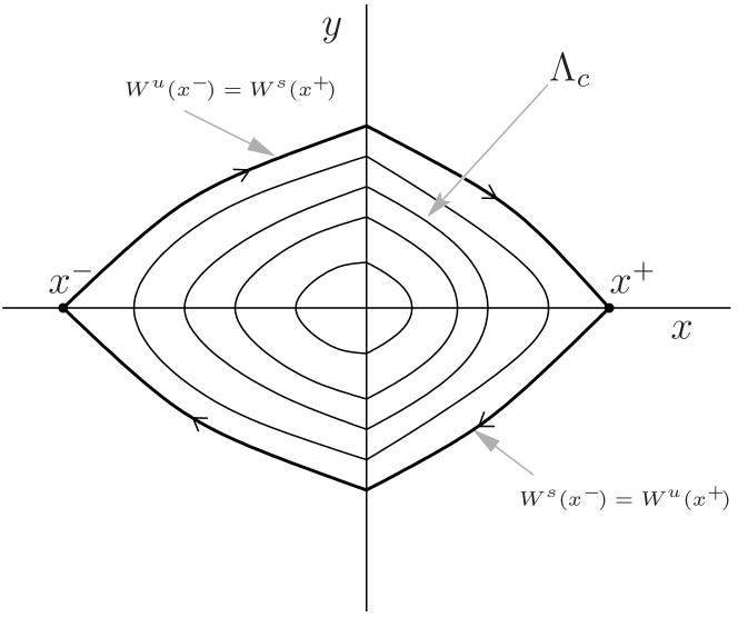
Figure 1: Phase portrait for the unperturbed system (2.2).

2.2 Poincaré impact map

To study system (2.2) we will proceed as in [Hog89] using the Poincaré impact map. We consider the extended phase space $\mathbb{R}^{2}\times\mathbb{R}$ adding time as a system variable and equation $\dot{t}=1$ to Eq. (2.2). As the perturbation is periodic, this time variable is usually defined in $\mathbb{T}=\mathbb{R}/T$; however, it will be more useful for us to consider $\mathbb{R}$ instead. We want to study the motion in the region surrounded by the heteroclinic orbit, so we consider in this extended phase-space the Poincaré section

$$\tilde{\Sigma}^{+}=\left\{(0,y,t)\in\mathbb{R}^{2}\times\mathbb{R}\,|\,0<y<\sqrt{2c_{1}}\right\}.$$ (2.8)

To simplify the notation, as the first coordinate in $\tilde{\Sigma}^{+}$ is always $0$, we will omit its repetition whenever this does not lead to confusion. The domain of the Poincaré map is not $\tilde{\Sigma}^{+}$ but a suitable open set $U$, that depends on $\varepsilon$ and, for $\varepsilon=0$, does not contain the heteroclinic connection.

We now define the Poincaré impact map

$$P_{\varepsilon}:U\subset\tilde{\Sigma}^{+}\longrightarrow\tilde{\Sigma}^{+},$$

as follows (see Fig. 2). First, using the section

$$\tilde{\Sigma}^{-}=\left\{(0,y,t)\in\mathbb{R}^{2}\times\mathbb{R}\,|\,-\sqrt{2c_{1}}<y<0\right\},$$ (2.9)

with $(0,y_{0},t_{0})\in U^{+}\subset\tilde{\Sigma}^{+}$, we define the map

$$P^{+}_{\varepsilon}:U^{+}\subset\tilde{\Sigma}^{+}\longrightarrow\tilde{\Sigma}^{-},$$

as

$$P^{+}_{\varepsilon}(y_{0},t_{0})=\left(\Pi_{y}\left(\phi^{+}\left(t_{1};t_{0},0,y_{0},\varepsilon\right)\right),t_{1}\right)$$ (2.10)

where $\phi^{+}(t;t_{0},x,y,\varepsilon)$ is the flow associated with system (2.2) restricted to $S^{+}$, and $t_{1}>t_{0}$ is the smallest value of $t$ satisfying the condition

$$\Pi_{x}\left(\phi^{+}\big{(}t_{1};t_{0},0,y_{0},\varepsilon\big{)}\right)=0.$$ (2.11)

Similarly, we consider

$$P^{-}_{\varepsilon}:U^{-}\subset\tilde{\Sigma}^{-}\longrightarrow\tilde{\Sigma}^{+}$$

for $(0,y_{1},t_{1})\in U^{-}\subset\tilde{\Sigma}^{-}$ defined by

$$P^{-}_{\varepsilon}(y_{1},t_{1})=\left(\Pi_{y}\left(\phi^{-}\left(t_{2};t_{1},0,y_{1},\varepsilon\right)\right),t_{2}\right)$$ (2.12)

where $\phi^{-}(t;t_{1},x,y,\varepsilon)$ is the flow associated with (2.2) restricted to $S^{-}$, and $t_{2}>t_{1}$ is the smallest value of $t$ satisfying the condition

$$\Pi_{x}\left(\phi^{-}\big{(}t_{2};t_{1},0,y_{1},\varepsilon\big{)}\right)=0.$$ (2.13)

Then the Poincaré impact map is defined as the composition

$$\begin{array}[]{cccc}P_{\varepsilon}:&U\subset\tilde{\Sigma}^{+}&\longrightarrow&\tilde{\Sigma}^{+}\\ &{\text{\footnotesize($y_{0},t_{0})$}}&\longmapsto&\text{\footnotesize$P_{\varepsilon}^{-}\!\!\circ\!P_{\varepsilon}^{+}\!(y_{0},t_{0})$}\\ \end{array}$$ (2.14)

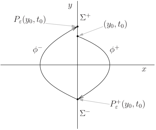
Figure 2: Poincaré impact map (2.14) represented schematically.

Notice that, as assumed in C.4, for the unperturbed flow all initial conditions in $\Sigma^{+}$ lead to periodic orbits surrounding the origin. Hence, we can give a closed expression for $P_{0}$, the Poincaré impact map when $\varepsilon=0$. Let

$$\alpha^{\pm}(\pm y)=\pm 2\mspace{-30.0mu}\mathop{\int}_{0}^{(V^{\pm})^{-1}(h)}\mspace{-30.0mu}\frac{1}{\sqrt{2(h-V^{\pm}(x))}}dx,\quad h=H_{0}(0,\pm y)=\frac{y^{2}}{2}$$ (2.15)

be the time needed by an orbit of the unperturbed system with initial condition $(0,\pm y)\in\Sigma^{\pm}$ to reach $\Sigma^{\mp}$. In the unperturbed case, the orbit with initial condition $(0,y)\in\Sigma^{+}$ has period

$$\alpha(y)=\alpha^{+}(y)+\alpha^{-}(-y).$$ (2.16)

Then the Poincaré impact map when $\varepsilon=0$ is defined in the whole $\tilde{\Sigma}^{+}$, and can be written as

$$P_{0}(y_{0},t_{0})=(y_{0},t_{0}+\alpha(y_{0})).$$ (2.17)

Thus, if $\varepsilon$ is small enough, the perturbed trajectories starting at $\tilde{\Sigma}^{+}$ cross $\tilde{\Sigma}^{+}$ again. The Poincaré impact map is well defined, and is as smooth as the flow restricted to $S^{+}$ and $S^{-}$.
Note that in the symmetric case, $V^{+}(x)=V^{-}(-x)$, $\alpha^{+}(y)=\alpha^{-}(-y)$ is half the period of the unperturbed periodic orbit with initial condition $(0,y)\in\Sigma^{+}$.

2.3 Coefficient of restitution

As the name of the previous map suggests, it is typically used to deal with systems with impacts, as is the case of the mechanical example of section 5. In order to include the loss of energy at the impact, one considers a coefficient of restitution, $r\in(0,1]$, that reduces the velocity, $y$, at every impact. More precisely, if a trajectory crosses $\Sigma$ transversally at some point $(0,y_{B})$ at $t=t_{B}$, then the state is replaced by $(0,ry_{B})$ at a later time $t_{A}$ to proceed with the evolution of the system. In other words, the system slides along $\Sigma$ from $(0,y_{B})$ to $(0,ry_{B})$ during time $t_{A}-t_{B}$ and

$$y(t_{A})=ry(t_{B}).$$ (2.18)

For the rest of this article we will assume that the loss of energy is produced instantaneously and hence $t_{A}=t_{B}$. Thus, there is no sliding along $\Sigma$ and the trajectory jumps from $(0,y_{B})$ to $(0,ry_{B})$.

Clearly, when such a condition is introduced to a system of the type (2.2), the unperturbed system ($\varepsilon=0$) is no longer conservative, the origin becomes a global attractor and none of the conditions C.1–C.5 hold. In particular, the orbits with initial conditions on the unstable manifolds $W^{u}(z^{-})$ and $W^{u}(z^{+})$ tend to the origin and can not intersect the stable manifolds $W^{s}(z^{+})$ and $W^{s}(z^{-})$, respectively (see Fig. 3).

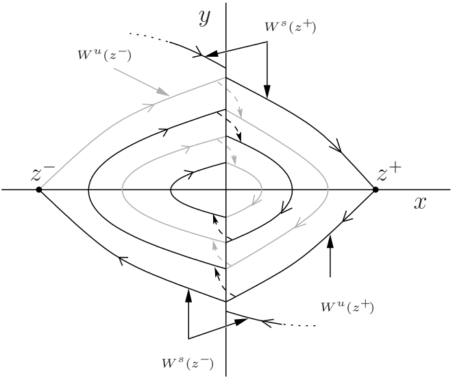
Figure 3: Stable and unstable manifolds of system (2.2) for $r<1$ and $\varepsilon=0$.

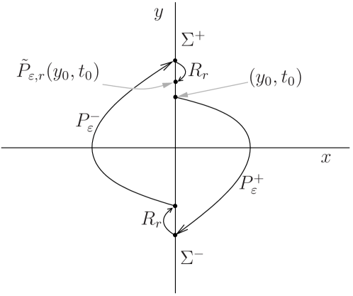
Figure 4: Impact map for $r<1$ and $\varepsilon>0$.

Although periodic orbits surrounding the origin are not possible for the unperturbed case if $r<1$, they may exist if $\varepsilon>0$. However, roughly speaking, as these orbits will have to overcome the loss of energy, the magnitude of the forcing will not be allowed to be arbitrarily small. We will make a precise statement of this fact in §3.2 (see also [Hog89]).

To study the existence of periodic orbits we will use again the impact map, which can also be defined for $r<1$ as (see Fig. 4)

$$\tilde{P}_{\varepsilon,r}(y_{0},t_{0}):=R_{r}\circ P_{\varepsilon}^{-}\circ R_{r}\circ P_{\varepsilon}^{+}(y_{0},t_{0})$$ (2.19)

where

$$R_{r}(y_{0},t_{0})=(ry_{0},t_{0}).$$

Note that $\tilde{P}_{\varepsilon,r}$ is as smooth as the flow restricted to $S^{\pm}$, since it is the composition of smooth maps.

Using Eqs. (2.15) and (2.16), the impact map, $\tilde{P}_{\varepsilon,r}$, for $\varepsilon=0$ and $r<1$ can be written as

$$\tilde{P}_{0,r}(y_{0},t_{0})=\left(r^{2}y_{0},t_{0}+\alpha^{+}\left(y_{0}\right)+\alpha^{-}(-ry_{0})\right).$$ (2.20)

Note that, for any $\varepsilon>0$,

$$\tilde{P}_{\varepsilon,1}(y_{0},t_{0})=P_{\varepsilon}(y_{0},t_{0}).$$

2.4 Some formal definitions and notation

Up to now, we have considered separately the solutions of system (2.2) in $S^{+}$ and $S^{-}$until they reach the switching manifold $\Sigma$. Given an initial condition $(x_{0},y_{0},t_{0})$, one can extend the definition of a solution, $\phi(t;t_{0},x_{0},y_{0},\varepsilon,r)$, of system (2.2),(2.18) for all $t\geq t_{0}$ by properly concatenating $\phi^{+}$ or $\phi^{-}$ whenever the flow crosses $\Sigma$ transversally. Depending on the sign of $x_{0}$, one applies either $\phi^{+}(t;t_{0},x_{0},y_{0},\varepsilon)$ or $\phi^{-}(t;t_{0},x_{0},y_{0},\varepsilon)$ until the trajectory reaches $\Sigma$, and then one applies (2.18). If $x_{0}=0$, one proceeds similarly depending on the sign of $y_{0}$. This is because $\dot{x}=y+O(\varepsilon)$ is always an equation of the flow and the orbits twist clockwise.

In this work, we will mainly use solutions with initial conditions $(0,y_{0},t_{0})\in\tilde{\Sigma}^{+}$. In that case, we define the sequence of impacts $(0,y_{\varepsilon,r}^{i},t_{\varepsilon,r}^{i})$ (see Fig. 5), if they exist, as

$$(y^{i}_{\varepsilon,r},t^{i}_{\varepsilon,r})=\left\{\begin{array}[]{ll}R_{r}\circ P_{\varepsilon}^{-}(y^{i-1}_{\varepsilon,r},t^{i-1}_{\varepsilon,r})&\text{if }y^{i-1}_{\varepsilon,r}<0\\ R_{r}\circ P_{\varepsilon}^{+}(y^{i-1}_{\varepsilon,r},t^{i-1}_{\varepsilon,r})&\text{if }y^{i-1}_{\varepsilon,r}>0\end{array}\right.,$$ (2.21)

with $(y^{0}_{\varepsilon,r},t^{0}_{\varepsilon,r})=(y_{0},t_{0})$ and $P_{\varepsilon}^{\pm}$ defined in (2.10) and (2.12). Notice that the sequence (2.21) will be finite if the flow reaches $\Sigma$ a finite number of times only.
For the unperturbed case, for any point $\left(0,y_{0},t_{0}\right)\in\tilde{\Sigma}^{+}$, the sequence (2.21) becomes

$$(y^{i}_{0,r},t^{i}_{0,r}):=\left\{\begin{array}[]{ll}\left(r^{i}y_{0},t_{0,r}^{i-1}+\alpha^{-}\left(-r^{i-1}y_{0}\right)\right)&\text{if }i\geq 2\text{ even}\\ \left(-r^{i}y_{0},t_{0,r}^{i-1}+\alpha^{+}\left(r^{i-1}y_{0}\right)\right)&\text{if }i\geq 1\text{ odd}\end{array}\right.,$$ (2.22)

where $\alpha^{\pm}$ are defined in Eq. (2.15).

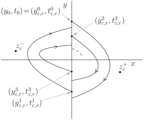
Figure 5: Sequence of impacts for $r<1$ and $\varepsilon>0$.

Once the impacts $(y_{\varepsilon,r}^{i},t_{\varepsilon,r}^{i})$ are defined, the solution of the non-autonomous system (2.2),(2.18) with initial condition $(0,y_{0},t_{0})\in\tilde{\Sigma}^{+}$ is given as

$$\phi(t;t_{0},0,y_{0},\varepsilon,r):=\left\{\begin{array}[]{ll}\phi^{+}(t;t_{\varepsilon,r}^{2i},0,y_{\varepsilon,r}^{2i},\varepsilon)&\text{if }t_{\varepsilon,r}^{2i}\leq t<t^{2i+1}_{\varepsilon,r}\\ \\ \phi^{-}(t;t_{\varepsilon,r}^{2i+1},0,y_{\varepsilon,r}^{2i+1},\varepsilon)&\text{if }t_{\varepsilon,r}^{2i+1}\leq t<t_{\varepsilon,r}^{2i+2}\end{array}\right.,\;i\geq 0.$$ (2.23)

Note that in the case when the number of impacts is finite, we take the last interval of time to be infinitely long.

In the rest of the paper we will generally distinguish between the conservative ($r=1$) and dissipative ($r<1$) cases. We will omit the parameter $r$ in the flow $\phi$ whenever we refer to $r=1$.
Note that we have only defined the solution of the system for an initial condition $(0,y_{0},t_{0})\in\tilde{\Sigma}^{+}$. Given $(0,y_{0},t_{0})\in\tilde{\Sigma}^{-}$, one defines similarly this solution by just properly shifting the subscripts of $t_{\varepsilon}^{i}$ in (2.23). In addition, it is possible to extend precisely this definition to an arbitrarily initial condition $(x_{0},y_{0},t_{0})$.

As is usual when dealing with Hamiltonian systems, we will use the unperturbed Hamiltonian to measure the distance between states. In addition, as we are dealing with a perturbation problem, we will frequently use expansions in powers of $\varepsilon$. In this case, the integral of the Poisson brackets of the Hamiltonians $H_{1}$ and $H_{0}$ typically provides a compact expression for the linear terms in $\varepsilon$. Given $m\geq 1$, $(0,y_{0},t_{0})\in\tilde{\Sigma}^{+}$ and its impact sequence $(0,y^{i}_{\varepsilon,r},t_{\varepsilon,r}^{i})$, $0\leq i\leq 2m$, for the non-smooth system (2.2),(2.18) when $r\leq 1$, we introduce

$$\int_{t_{0}}^{t_{\varepsilon,r}^{2m}}\left\{H_{0},H_{1}\right\} \left(\phi\left(t;t_{0},0,y_{0},\varepsilon,r\right),t\right)dt$$ (2.24)

$$:=\sum_{i=0}^{m-1}\Bigg{(}\int_{t_{\varepsilon,r}^{2i}}^{t_{\varepsilon,r}^{2i+1}}\left\{H_{0}^{+},H_{1}^{+}\right\}\left(\phi^{+}(t;t_{\varepsilon,r}^{2i},0,y_{\varepsilon,r}^{2i},\varepsilon),t\right)dt$$

$$+\int_{t_{\varepsilon,r}^{2i+1}}^{t^{2i+2}_{\varepsilon,r}}\left\{H_{0}^{-},H_{1}^{-}\right\}\left(\phi^{-}(t;t_{\varepsilon,r}^{2i+1},0,y_{\varepsilon,r}^{2i+1},\varepsilon),t\right)dt\Bigg{)}$$

where $\left\{Q\left(x,y\right),R\left(x,y\right)\right\}=\frac{\partial Q}{\partial x}\frac{\partial R}{\partial y}-\frac{\partial Q}{\partial y}\frac{\partial R}{\partial x}$ is the usual Poisson bracket of the Hamiltonians $Q$ and $R$.

The next Lemma provides an expression for $H_{0}\left(\phi\left(t^{2m}_{\varepsilon,r};t_{0},0,y_{0},\varepsilon,r\right)\right)$ which we will use below.

Lemma 1.

Let $m\geq 1$ and $(0,y_{0},t_{0})\in\tilde{\Sigma}^{+}$, and let $(0,y^{i}_{\varepsilon,r},t^{i}_{\varepsilon,r})$, $i=0,\dots,2m$, be its associated impact sequence as defined in (2.21). Then,

$$H_{0}(0,y_{\varepsilon,r}^{2m}) -H_{0}\left(0,y_{0}\right)=r^{2}\Bigg{[}\varepsilon\int_{t_{0}}^{t_{\varepsilon,r}^{2m}}\left\{H_{0},H_{1}\right\}\left(\phi\left(t;t_{0},0,y_{0},\varepsilon,r\right),t\right)dt$$ (2.25)

$$+\sum_{i=0}^{2m-1}\left(H_{0}\left(0,y^{i}_{\varepsilon,r}\right)-H_{0}\left(0,\frac{y^{i}_{\varepsilon,r}}{r}\right)\right)\Bigg{]}.$$

Proof.

The proof of this Lemma comes from a straightforward application of the fundamental theorem of calculus to the smooth functions $H_{0}^{\pm}\left(\phi^{\pm}\left(t;t_{0},0,\pm y_{0},\varepsilon\right)\right)$, using the fact that

$$H_{0}(0,y_{\varepsilon,r}^{2m}) =H_{0}\left(r\phi\left(t_{\varepsilon,r}^{2m};t_{0},0,y_{0},\varepsilon,r\right)\right)$$

$$=r^{2}H_{0}\left(\phi\left(t_{\varepsilon,r}^{2m};t_{0},0,y_{0},\varepsilon,r\right)\right),$$

taking into account the intermediate gaps induced by the impact condition (2.18) and using the fact that

$$\frac{d}{dt}H_{0}^{\pm}\left(\phi^{\pm}\left(t;t^{*},x^{*},y^{*},\varepsilon\right)\right)=\varepsilon\left\{H_{0}^{\pm},H_{1}^{\pm}\right\}\left(\phi^{\pm}\left(t;t^{*},x^{*},y^{*},\varepsilon\right)\right)$$

for any $(x^{*},y^{*})\in S^{\pm}\cup\Sigma^{\pm}$ and $t\geq t^{*}$ such that $\phi^{\pm}\left(t;t^{*},x^{*},y^{*},\varepsilon\right)\in S^{\pm}$. ∎

The following Lemma gives us an expression for the expansion in powers of $\varepsilon$ of $H_{0}(0,y_{\varepsilon,r}^{2m})-H_{0}\left(0,y_{0}\right)$ which we will use in §3.

Lemma 2.

Let $m\geq 1$ and $(0,y_{0},t_{0})\in\tilde{\Sigma}^{+}$, and let $(0,y^{i}_{\varepsilon,r},t^{i}_{\varepsilon,r})$, $i=0,\dots,2m$, be its associated impact sequence as defined in (2.21). Then, if $\varepsilon\simeq 0$, the Taylor expansion of expression (2.25) becomes

$$H_{0}(0,y_{\varepsilon,r}^{2m})-H_{0}\left(0,y_{0}\right) =\frac{y_{0}^{2}}{2}(r^{4m}-1)+\varepsilon G^{m}(y_{0},t_{0})$$ (2.26)

$$+O(\varepsilon^{2})+O(\varepsilon\left(r-1\right))$$

where

$$G^{m}(y_{0},t_{0})=\int_{0}^{m\alpha(y_{0})}\left\{H_{0},H_{1}\right\}\left(\phi\left(t;0,0,y_{0},0\right),t+t_{0}\right)dt$$ (2.27)

and $\alpha(y_{0})$ is given in (2.16).

Proof.

The independent term of the expansion is found by noting that, if $\varepsilon=0$, from expression (2.22), one has $H_{0}(0,y^{i}_{0,r})=H_{0}(0,\frac{y^{i+1}_{0,r}}{r})$. Hence all the terms in the sum of Eq. (2.25) cancel each other except for the first and the last one. This, in combination with the fact that $H_{0}(0,y)=\frac{y^{2}}{2}$, gives the first term in Eq. (2.26). For the linear term in $\varepsilon$, one first obtains

$$r^{2}\Bigg{[}\int_{t_{0}}^{t_{\varepsilon,r}^{2m}}\left\{H_{0},H_{1}\right\}\left(\phi\left(t;t_{0},0,y_{0},0,r\right),t\right)dt$$

$$+(r^{2}-1)\sum_{i=1}^{2m-1}\left(\frac{d}{d\varepsilon}\left(H_{0}\left(\left(y_{\varepsilon,r}^{i},t_{\varepsilon,r}^{i}\right)\right)\right)_{|\varepsilon=0}\right)\Bigg{]}.$$

Then, by applying $m$ times Eq. (2.20), one has that $t_{\varepsilon,1}^{2m}=t_{0}+m\alpha(y_{0})+O(\varepsilon)$. Thus, by expanding this for $r$ near $1$ and $\varepsilon$ near $0$ and noting that the unperturbed flow is autonomous and hence $\phi(t;t_{0},0,y_{0},0)=\phi(t-t_{0};0,0,y_{0},0)$, one gets expression (2.27). ∎

Remark 1.

If in Eq. (2.27) we take $\alpha(y_{0})=\frac{nT}{m}$, then we recover the classical Melnikov function for the subharmonic orbits [GH83] with the modified integral (2.24).

3 Existence of subharmonic orbits

3.1 Conservative case, $r=1$: Melnikov method for subharmonic orbits

Let us consider system (2.2) neglecting the loss of energy at impact ($r=1$ in Eq. (2.18)). According to C.1–C.5, for $\varepsilon=0$, this system possesses a continuum of periodic orbits, $\Lambda_{c}$ in Eq. (2.7), surrounding the origin. Our main goal in this section is to investigate the persistence of these orbits when the (periodic) non-autonomous perturbation is considered ($\varepsilon>0$). The classical Melnikov method for subharmonic orbits, which here, in principle, does not apply, provides sufficient conditions for the persistence of periodic orbits for a smooth system with an equivalent, smooth, unperturbed phase portrait.

The period of the orbits $\Lambda_{c}$ tends to infinity as they approach the heteroclinic orbit. More precisely, if $q_{c}(t)$ is the periodic orbit satisfying $q_{c}(0)=(0,y_{0})$ with $H_{0}(0,y_{0})=c$, its period $\alpha(y_{0})$ tends to infinity as $c\to c_{1}$ (see formula (2.16)). As we are interested in finding periodic orbits for $0<\varepsilon\ll 1$, we will use the unperturbed periodic solutions as $\varepsilon$-close approximations to them. In general, such perturbation results are valid only for finite time and therefore, from now on, we will restrict ourselves to a set of the form

$$\tilde{\Sigma}^{+}_{\tilde{c}}=\left\{(0,y,t)\in\tilde{\Sigma}^{+}\,|\,0\leq y\leq\tilde{c}\right\},$$ (3.1)

for a fixed $\tilde{c}$ satisfying $0\leq\tilde{c}<\sqrt{2c_{1}}$. Note that, if $(0,y_{0},t_{0})\in\tilde{\Sigma}_{\tilde{c}}^{+}$ then $\alpha(y_{0})$ is uniformly bounded ($\alpha(y_{0})<\alpha(\tilde{c})$). However, following [GH83], it is also possible to extend the method for all the periodic orbits up to the heteroclinic connection.

To look for periodic orbits we will use the impact map defined in (2.14). In terms of this map, a point in $U\subset\tilde{\Sigma}^{+}$ will lead to a periodic orbit of period $nT$ if it is a solution of the equation

$$P^{m}_{\varepsilon}(y_{0},t_{0})=(y_{0},t_{0}+nT),$$ (3.2)

for some $m$. We take $m$ to be the smallest integer such that (3.2) is satisfied. In that case, $\phi\left(t;t_{0},0,y_{0},\varepsilon\right)$ will be a periodic orbit of period $nT$, which crosses the switching manifold $\Sigma$ exactly $2m$ times. We will call this an $(n,m)$-periodic orbit. Then for $(n,m)$-periodic orbits with $\varepsilon>0$ we have the following result analogous to the smooth case

Theorem 1.

Consider a system as defined in (2.2) satisfying C.1–C.5, and let $\alpha(y_{0})$ be the function defined in (2.15)-(2.16). Assume that the point $(0,\bar{y}_{0},\bar{t}_{0})\in\tilde{\Sigma}_{\tilde{c}}^{+}$ satisfies

1. $\alpha(\bar{y}_{0})=\frac{n}{m}T$, with $n,m\in\mathbb{Z}$ relatively prime

2. $\bar{t}_{0}\in[0,T]$ is a simple zero of

   $$M^{n,m}(t_{0})=\int_{0}^{nT}\left\{H_{0},H_{1}\right\}(q_{c}(t),t+t_{0})dt,\;c=H_{0}(0,\bar{y}_{0}),$$ (3.3)

where $q_{c}(t)=\phi\left(t;0,0,\bar{y}_{0}\right)$ is the periodic orbit such that $\alpha(\bar{y}_{0})=\frac{nT}{m}$.
Then, there exists $\varepsilon_{0}$ such that, for every $0<\varepsilon<\varepsilon_{0}$, one can find $y_{0}^{*}$ and $t_{0}^{*}$ such that $\phi(t;t_{0}^{*},0,y_{0}^{*},\varepsilon)$ is an $(n,m)$-periodic orbit.

Proof.

The proof of the result comes from a straightforward application of the implicit function theorem to equation (3.2). Let us fix $n$ and $m$ relatively prime. We replace equation (3.2) by

$$\left(\begin{array}[]{c}H_{0}\left(0,\Pi_{y_{0}}(P_{\varepsilon}^{m}(y_{0},t_{0}))\right)\\ \Pi_{t_{0}}\left(P^{m}_{\varepsilon}(y_{0},t_{0})\right)\end{array}\right)-\left(\begin{array}[]{c}H_{0}(0,y_{0})\\ t_{0}+nT\end{array}\right)=\left(\begin{array}[]{c}0\\ 0\end{array}\right).$$ (3.4)

That is, we use the Hamitlonian $H_{0}$ to measure the distance between the points $\left(0,\Pi_{y_{0}}\left(P^{m}_{\varepsilon}\left(y_{0},t_{0}\right)\right)\right)$ and $\left(0,y_{0}\right)$.
Using the second equation in (3.4) we have

$$\Pi_{y_{0}}\left(P_{\varepsilon}^{m}\left(y_{0},t_{0}\right)\right) =\Pi_{y}\left(\phi(t_{0}+nT;t_{0},0,y_{0},\varepsilon)\right)$$

$$0 =\Pi_{x}\left(\phi\left(t_{0}+nT;t_{0},0,y_{0},\varepsilon\right)\right).$$

This allows us to rewrite Eq. (3.4) as

$$\left(\begin{array}[]{c}H_{0}(\phi(t_{0}+nT;t_{0},0,y_{0},\varepsilon))-H_{0}(0,y_{0})\\ \Pi_{t_{0}}\left(P_{\varepsilon}^{m}\left(y_{0},t_{0}\right)\right)-nT-t_{0}\end{array}\right)=\left(\begin{array}[]{c}0\\ 0\end{array}\right).$$ (3.5)

We expand Eq. (3.5) in powers of $\varepsilon$. Using Eq. (2.17), the second component of (3.5) becomes

$$\Pi_{t_{0}}\left(P^{m}_{\varepsilon}\left(y_{0},t_{0}\right)\right)-t_{0}-nT=m\alpha(y_{0})-nT+O(\varepsilon)=0,$$ (3.6)

where $\alpha(y_{0})$ is the period of the periodic orbit $q_{c}(t)$, $c=H_{0}(0,y_{0})$, given in Eq. (2.16).
On the other hand, using Lemma 2 and noting that

$$\Pi_{y_{0}}\left(P_{\varepsilon}^{m}\left(y_{0},t_{0}\right)\right)=y_{\varepsilon,1}^{2m},$$

the first equation in (3.5) can be written as

$$H_{0}(0,\Pi_{y_{0}} (P_{\varepsilon}^{m}(y_{0},t_{0})))-H_{0}(0,y_{0})$$

$$=\varepsilon\int_{0}^{m\alpha(y_{0})}\left\{H_{0},H_{1}\right\}(\phi(t;0,0,y_{0},0),t+t_{0})dt+O(\varepsilon^{2})$$

$$=\varepsilon G^{m}(y_{0},t_{0})+O(\varepsilon^{2}).$$

where $G^{m}(y_{0},t_{0})$ is given in (2.27). Hence, Eq. (3.5) finally becomes

$$F_{n,m}(y_{0},t_{0},\varepsilon):=\left(\begin{array}[]{c}G^{m}(y_{0},t_{0})+O(\varepsilon)\\ m\alpha(y_{0})-nT+O(\varepsilon)\\ \end{array}\right)=\left(\begin{array}[]{c}0\\ 0\end{array}\right),$$ (3.7)

where the order in $\varepsilon$ of the first component has been reduced and, thus, the implicit function theorem can be applied to Eq. (3.7). Therefore, one needs

1. $F_{n,m}(\bar{y}_{0},\bar{t}_{0},0)=(0,0)^{T}$

2. $\det(D_{y_{0},t_{0}}F(\bar{y}_{0},\bar{t}_{0},0))\neq 0$, where $D_{y_{0},t_{0}}\equiv D$ is the Jacobian with respect to the variables $y_{0}$ and $t_{0}$.

The first condition is satisfied by noting in Eq. (3.7) that $\bar{y}_{0}$ has to be such that $\alpha(\bar{y}_{0})=\frac{nT}{m}$ and $\bar{t}_{0}$ a zero of the subharmonic Melnikov function

$$M^{n,m}(t_{0}):=G^{m}(\bar{y}_{0},t_{0})=\int_{0}^{nT}\left\{H_{0},H_{1}\right\}(q_{c}(t),t+t_{0})dt,$$

where $q_{c}(t)$, $c=H_{0}(0,\bar{y}_{0})$, is the unperturbed periodic orbit of period $\frac{nT}{m}$ such that $q_{c}(0)=(0,y_{0})$, and therefore $q_{c}(t)=\phi\left(t;0,0,\bar{y}_{0},0\right)$.
In addition, for $\varepsilon=0$, $DF_{n,m}$ is given by

$$DF_{n,m}(y_{0},t_{0},0)=\left(\begin{array}[]{cc}\frac{\partial G^{m}}{\partial y_{0}}&\frac{\partial G^{m}}{\partial t_{0}}\\ m\alpha^{\prime}(y_{0})&0\end{array}\right).$$

By C.5, $\alpha^{\prime}(y_{0})\neq 0$, and the second condition is satisfied if $\bar{t}_{0}$ is a simple zero of the subharmonic Melnikov function, $M^{n,m}(t_{0})$, which completes hypothesis H.2.
Finally, applying the implicit function theorem to (3.7) at $(y_{0},t_{0},\varepsilon)=(\bar{y}_{0},\bar{t}_{0},0)$, there exists $\varepsilon_{0}>0$ such that, if $0<\varepsilon<\varepsilon_{0}$, then there exist unique $y_{0}^{*}(\varepsilon)$ and $t_{0}^{*}(\varepsilon)$ solutions of the equation (3.4), which have the form

$$y_{0}^{*}=\bar{y}_{0}+O(\varepsilon)$$

$$t_{0}^{*}=\bar{t}_{0}+O(\varepsilon).$$

Hence, the orbit $\phi\left(t;t^{*}_{0},0,y^{*}_{0},\varepsilon\right)$ is an $(n,m)$-periodic orbit, as it has period $nT$ and impacts $2m$ times with the switching manifold $\Sigma$ in every period. ∎

Remark 2.

The upper bound $\varepsilon_{0}$ given in the theorem depends on $n$ and $m$. However, for every fixed $m$, it is possible to obtain $\varepsilon_{0}(m)$, such that for $\varepsilon<\varepsilon_{0}(m)$, we can apply the theorem for all $n$ such that $\alpha^{-1}(\frac{nT}{m})\in\tilde{\Sigma}_{\tilde{c}}^{+}$. This is because the approximation of the perturbed flow by the unperturbed periodic orbit is performed $m$ times beyond the period of the unperturbed periodic orbit.

Remark 3.

The proof of the result provides us with a constructive method to find the initial condition for $nT$-periodic orbits for $\varepsilon>0$.

1. Given $n$ and $m$, find $\bar{y}_{0}$ such that $\alpha(\bar{y}_{0})=\frac{n}{m}T$ using Eq. (2.16).

2. Find $\bar{t}_{0}$ such that $M^{n,m}(t_{0})$ has a simple zero at $t_{0}=\bar{t}_{0}$.

3. Use $(\bar{y}_{0},\bar{t}_{0})$ as seed to solve Eq. (3.4) numerically.

Lemma 3.

The subharmonic Melnikov function (3.3) is either identically zero or generically possesses at least one simple zero.

Proof.

The proof comes from the fact that $M^{n,m}(t_{0})$ has average

$$<M^{n,m}(t_{0})>=\frac{1}{T}\int_{0}^{T}M^{n,m}(t_{0})dt_{0}$$

equal to zero.

$$<M^{n,m}(t_{0})> =\frac{1}{T}\int_{0}^{T}\int_{0}^{nT}\left\{H_{0},H_{1}\right\}\left(q_{c}(t),t+t_{0}\right)dtdt_{0}$$

$$=\frac{1}{T}\int_{0}^{nT}\int_{0}^{T}\left\{H_{0},H_{1}\right\}\left(q_{c}(t),t+t_{0}\right)dt_{0}dt$$

$$=\int_{0}^{nT}\left\{H_{0},<H_{1}>\right\}(q_{c}(t))dt.$$

Recalling that $\alpha(y_{0})=\frac{nT}{m}$ (see (2.15)-(2.16)) and letting

$$q_{c}^{+}(t)=\phi^{+}(t;0,0,y_{0},0)$$

$$q_{c}^{-}(t)=\phi^{-}(t;\alpha^{+}(y_{0}),0,-y_{0},0),$$

$<M^{n,m}(t_{0})>$ can be written as

$$m\left(\int_{0}^{\alpha^{+}(y_{0})}\left\{H_{0}^{+},<H_{1}^{+}>\right\}\left(q_{c}^{+}(t)\right)dt+\int_{\alpha^{+}(y_{0})}^{\frac{nT}{m}}\left\{H_{0}^{-},<H_{1}^{-}>\right\}\left(q_{c}^{-}(t)\right)dt\right)$$

$$=-m\left(\int_{0}^{\alpha^{+}(y_{0})}\frac{d}{dt}\left(<H_{1}^{+}>\left(q_{c}^{+}(t)\right)\right)dt+\int_{\alpha^{+}(y_{0})}^{\frac{nT}{m}}\frac{d}{dt}\left(<H_{1}^{-}>\left(q_{c}^{-}(t)\right)\right)dt\right)$$

$$=-m\Bigg{(}<H_{1}^{+}>\left(q_{c}^{+}(\alpha^{+}(y_{0}))\right)-<H_{1}^{+}>\left(q_{c}^{+}(0)\right)$$

$$+<H_{1}^{-}>\left(q_{c}^{-}({\textstyle\frac{nT}{m}})\right)-<H_{1}^{-}>\left(q_{c}^{-}\left(\alpha^{+}(y_{0})\right)\right)\Bigg{)}=0.$$

∎

Note that, if $M^{n,m}(t_{0})\equiv 0$ then a second order analysis is required to study the existence of periodic orbits.

3.2 Dissipative case, $r<1$

We now focus on the situation when the coefficient of restitution $r$ introduced in §2.3 is considered. As already mentioned, for $\varepsilon=0$ the origin is a global attractor and hence none of the periodic orbits studied in the previous section exists if the amplitude of the perturbation is small enough. However, as was shown in [Hog89] for the rocking block model, for $\varepsilon$ large enough an infinite number periodic orbits surrounding the origin can exist. This was studied analytically and numerically for the rocking block model under symmetry assumptions for the particular case $m=1$. Here, our goal is to relate the periodic orbits existing for the dissipative case to those which exist for $r=1$ in the general system (2.2),(2.18). As will be shown below, all the periodic orbits given by Theorem 1 can also exist for the dissipative case, when $r<1$ is small enough compared with $\varepsilon>0$. In other words, we generalise in this section the result presented for the conservative case.

As in §3.1, in order to obtain the initial conditions of a $(n,m)$-periodic orbit for $r<1$, one has to solve the equation

$$\tilde{P}^{m}_{\varepsilon,r}(y_{0},t_{0})=(y_{0},t_{0}+nT),$$ (3.8)

where $\tilde{P}_{\varepsilon,r}$, is defined in Eq. (2.19). The next result states that, under certain conditions regarding $r$ and $\varepsilon$, Eq. (3.8) can be solved.

Theorem 2.

Consider system (2.2),(2.18). Let $(0,\bar{y}_{0},\bar{t}_{0})\in\tilde{\Sigma}^{+}$ be such that $\alpha(\bar{y}_{0})=\frac{nT}{m}$, with $n$ and $m$ relatively prime, and $\bar{t}_{0}$ a simple zero of the subharmonic Melnikov function (3.3). There exists $\rho$ such that, given $\tilde{\varepsilon},\tilde{r}>0$ satisfying $0<\frac{\tilde{r}}{\tilde{\varepsilon}}<\rho$, there exists $\delta_{0}$ such that, if $\varepsilon=\tilde{\varepsilon}\delta$ and $r=1-\tilde{r}\delta$, then $\forall\,0<\delta<\delta_{0}$ there exists $(y_{0}^{*},t_{0}^{*})$ which is a solution of Eq. (3.8). Moreover, $y_{0}^{*}=\bar{y}_{0}+O(\delta)$, $t_{0}^{*}=\bar{t}_{0}+O(\delta)+O(\tilde{r}/\tilde{\varepsilon})$ and the solution $(y_{0}^{*},t_{0}^{*})$ tends to the one given in Theorem 1 as $r\to 1^{-}$.

Proof.

As in the conservative case, we use the unperturbed Hamiltonian to measure the distance between points in $\Sigma$. Then, Eq. (3.8) can be rewritten as

$$\left(\begin{array}[]{c}H_{0}\left(0,\Pi_{y_{0}}(\tilde{P}_{\varepsilon}^{m}(y_{0},t_{0}))\right)\\ \Pi_{t_{0}}\left(\tilde{P}^{m}_{\varepsilon}(y_{0},t_{0})\right)\end{array}\right)-\left(\begin{array}[]{c}H_{0}(0,y_{0})\\ t_{0}+nT\end{array}\right)=\left(\begin{array}[]{c}0\\ 0\end{array}\right).$$ (3.9)

As in Theorem 1, we proceed by expanding this equation in powers of $\varepsilon$ and $r-1$ using (2.26) and (2.27) obtaining

$$\left(\begin{array}[]{c}\frac{y_{0}^{2}}{2}(r^{4m}-1)+\varepsilon G^{m}(y_{0},t_{0})+O(\varepsilon^{2})+O(\varepsilon(r-1))\\ \displaystyle\sum_{i=0}^{m-1}\alpha^{+}(r^{2i}y_{0})+\sum_{i=0}^{m-1}\alpha^{-}\left(-r^{2i+1}y_{0}\right)+O(\varepsilon)-nT\end{array}\right)=\left(\begin{array}[]{c}0\\ 0\end{array}\right).$$ (3.10)

Note that, for $r=1$, Eq. (3.10) becomes Eq. (3.5).

We are interested in studying Eq. (3.10) when $1-r$ and $\varepsilon$ are both small. Therefore, for $\tilde{\varepsilon}>0$ and $\tilde{r}>0$ we set

$$\varepsilon=\tilde{\varepsilon}\delta,\;r=1-\tilde{r}\delta,$$ (3.11)

where $\delta>0$ is a small parameter. Then Eq. (3.10) becomes

$$\tilde{F} {}_{n,m}(y_{0},t_{0},\delta):=$$

$$\left(\begin{array}[]{c}-2m\tilde{r}y_{0}^{2}+\tilde{\varepsilon}G^{m}(y_{0},t_{0})+O(\delta)\\ \displaystyle m\alpha(y_{0})+O(\delta)-nT\end{array}\right)=\left(\begin{array}[]{c}0\\ 0\end{array}\right).$$ (3.16)

We now need to apply the implicit function theorem to (3.16).
The first step is to solve Eq. (3.16) for $\delta=0$. The second equation gives $\alpha(\bar{y}_{0})=\frac{nT}{m}$, as in Theorem 1. To solve the first equation, we define

$$f^{n,m}(t_{0})=-2m\tilde{r}\bar{y}_{0}^{2}+\tilde{\varepsilon}M^{n,m}(t_{0}),$$ (3.17)

and $\widehat{t}_{0}$ will be given by a zero of $f^{n,m}(t_{0})$. Assume now that $\bar{t}_{0}$ is a simple zero of $M^{n,m}(t_{0})$. As $M^{n,m}(t_{0})$ is a smooth periodic function, it possesses at least one local maximum. Let $t_{M}$ be the closest value to $\bar{t}_{0}$ where $M^{n,m}(t_{0})$ possesses a local maximum, and assume $\left(M^{n,m}\right)^{\prime}(t_{0})\neq 0$ for all $t_{0}$ between $\bar{t}_{0}$ and $t_{M}$. If $\left(M^{n,m}\right)^{\prime}(t_{0})$ vanishes between $\bar{t}_{0}$ and $t_{M}$, we then take $t_{M}$ to be the closest value to $\bar{t}_{0}$ such that $\left(M^{n,m}\right)^{\prime}(t_{0})=0$ to ensure that $\left(M^{n,m}\right)^{\prime}(t_{0})\neq 0$ between $\bar{t}_{0}$ and $t_{M}$. We then define $\rho:=\frac{M^{n,m}(t_{M})}{2m\bar{y}_{0}^{2}}$. Then, if

$$0<\frac{\tilde{r}}{\tilde{\varepsilon}}<\rho,$$ (3.18)

there exists $\widehat{t}_{0}$ $\frac{\tilde{r}}{\tilde{\varepsilon}}$-close to $\bar{t}_{0}$ where $f^{n,m}(t_{0})$ has a simple zero. Since $\alpha^{\prime}(\bar{y}_{0})>0$, a similar calculation to the one in Theorem 1 shows that

$$\det\left(D\tilde{F}_{y_{0},t_{0}}\left(\bar{y}_{0},\widehat{t}_{0},0\right)\right)\neq 0,$$

and hence we can apply the implicit function theorem near $(y_{0},t_{0},\delta)=(\bar{y}_{0},\widehat{t}_{0},0)$ to show that there exists $\delta_{0}$ such that, if $0<\delta<\delta_{0}$, then there exists

$$(y_{0}^{*},t_{0}^{*})=(\bar{y}_{0},\widehat{t}_{0})+O(\delta)=\left(\bar{y}_{0},\bar{t}_{0}\right)+O(\delta)+O(\tilde{r}/\tilde{\varepsilon})$$

which is a solution of Eq. (3.8).
This solution tends to the one given by Theorem 1 when $\tilde{r}\to 0^{+}$ . This is a natural consequence of that fact that Eq. (3.8) tends to the Equation (3.2) as $r\to 1^{-}$. ∎

Remark 4.

In order to determine $\rho$, we have imposed $t_{M}$ to be the local maximum of the Melnikov function closest to its simple zero, $\bar{t}_{0}$. Instead, one could also use the absolute maximum so increasing the range given in Eq. (3.18). However, in this case, the values where $\left(M^{n,m}_{1}\right)^{\prime}(t_{0})=0$ have to be avoided to ensure that the desired zero of $f^{n,m}(t_{0})$ is simple.

Remark 5.

Arguing as in Remark 2, for every $m$ fixed, the constant $\delta_{0}(m)$ can be taken such that if $\delta<\delta_{0}(m)$, there exist periodic orbits for all $n$ such that $\alpha(\frac{nT}{m})^{-1}\in\tilde{\Sigma}$.

4 Intersection of the separatrices

We now focus our attention on the invariant manifolds of the saddle points of system (2.2),(2.18) when $\varepsilon>0$. As explained in §2, for $\varepsilon=0$, there exist two heteroclinic orbits connecting the critical points $z^{\pm}$ if $r=1$ (see Fig. 1) whereas, if $r<1$, the unstable manifolds $W^{u}(z^{\pm})$ spiral discontinuously from $z^{\pm}$ to the origin and $W^{s}(z^{\pm})$ becomes unbounded (see Fig. 3). As we will show, in both cases, heteroclinic orbits may exist for the perturbed system.

For a smooth system with Hamiltonian $K_{0}(x,y)+\varepsilon K_{1}(x,y,t)$, the persistence of homoclinic or heteroclinic connections is achieved by the well known Melnikov method which states that if the Melnikov function

$$M(t_{0})=\int_{-\infty}^{+\infty}\left\{K_{0},K_{1}\right\}\left(\phi\left(t;t_{0},z_{0},0\right),t+t_{0}\right)dt,$$

with $z_{0}=(x_{0},y_{0})\in W^{u}(z^{-})=W^{s}(z^{+})$, has a simple zero, then the stable and unstable manifolds intersect for $\varepsilon>0$ small enough (see [GH83]).
In this section we will modify the classical Melnikov method and we will rigorously prove that it is still valid for a piecewise smooth system of the form (2.2), even if $r\leq 1$.
There exist in the literature several works where this tool has been used in particular non-smooth examples, [Hog92, BK91]. Theorem 3 generalises the result stated in [BK91] where the Melnikov method is shown to work, although the proof there is not complete.
The homoclinic version of a piecewise-defined system with a different topology was studied in [Kun00], [Kuk07] and [BF08]. However, the tools developed there do not apply for a system of the type (2.2).

We begin by discussing the persistence of objects for $\varepsilon>0$ and $r\leq 1$. It is clear that by separately extending the systems $\mathcal{X}_{0}^{\pm}+\varepsilon\mathcal{X}_{1}^{\pm}$ to $\mathbb{R}^{2}\times\mathbb{T}$, where $\mathbb{T}=\mathbb{R}/T$, we get two smooth systems for which the classical perturbation theory holds. It follows then that, as $z^{\pm}$ are hyperbolic fixed points, for $\varepsilon>0$ small enough there exist two hyperbolic $T$-periodic orbits, $\Lambda^{\pm}_{\varepsilon}\equiv\{z_{\varepsilon}^{\pm}(\tau);\tau\in[0,T]\}$, with two-dimensional stable and unstable manifolds $W^{s,u}(\Lambda^{\pm}_{\varepsilon})$.

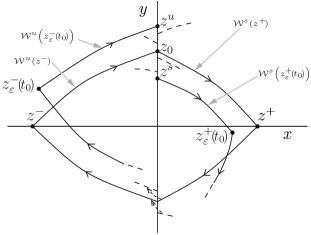
Figure 6: Section of the unperturbed and perturbed invariant manifolds for $t=t_{0}$.

As the system is non-autonomous, we fix the Poincaré section

$$\Theta_{t_{0}}=\left\{(x,y,t_{0}),\,(x,y)\in\mathbb{R}^{2}\right\},$$

and consider the time $T$ stroboscopic map

$$\Pi_{t_{0}}:\Theta_{t_{0}}\longrightarrow\Theta_{t_{0}+T},$$

where

$$\Pi_{t_{0}}(z)=\phi(t_{0}+T;t_{0},z,\varepsilon,r)$$

and $\phi$ is defined §2.4.
This map has $z^{\pm}_{\varepsilon}(t_{0})$ as hyperbolic fixed points with one dimensional stable and unstable manifolds $W^{s,u}(z^{\pm}_{\varepsilon}(t_{0}))$ (see Fig. 3). Proceeding as in [BK91], we fix the section $\Sigma$ defined in (2.1) and study its intersection with the stable and unstable curves $W^{u}(z_{\varepsilon}^{-}(t_{0}))$ and $W^{s}(z_{\varepsilon}^{+}(t_{0}))$. In the unperturbed conservative case ($\varepsilon=0$ and $r=1$), $W^{u}(z^{-})$ and $W^{s}(z^{+})$ intersect transversally $\Sigma$ in a point $z_{0}$. The perturbed manifolds, $W^{u}(z_{\varepsilon}^{-}(t_{0})$) and $W^{s}(z_{\varepsilon}^{+}(t_{0})$), intersect $\Sigma$ at points $z^{u}(t_{0})$ and $z^{s}(t_{0})$ respectively, $\varepsilon$-close to $z_{0}$ (see Fig. 6). Recalling the effect of the coefficient of restitution (2.18) explained in §2.3, both invariant manifolds will intersect if, for some $t_{0}$, one has $rz^{u}(t_{0})=z^{s}(t_{0})$, $r\leq 1$. As in [BK91] and [Hog92], we use the unperturbed Hamiltonian $H_{0}(x,y)$ to measure the distance $\Delta(t_{0},\varepsilon,r)$ between $z^{u}$ and $z^{s}$

$$\Delta(t_{0},\varepsilon,r)=H_{0}(rz^{u}(t_{0}))-H_{0}(z^{s}(t_{0}))=r^{2}H_{0}(z^{u}(t_{0}))-H_{0}(z^{s}(t_{0})).$$ (4.1)

We then have the following result.

Theorem 3.

Consider system (2.2),(2.18), and let $z_{0}=W^{s}(z^{+})\cap\Sigma$. Define the Melnikov function

$$M(t_{0})=\int_{-\infty}^{+\infty}\mspace{-10.0mu}\left\{H_{0},H_{1}\right\}\left(\phi\left(t;t_{0},z_{0},0\right),t\right)dt,$$ (4.2)

where

$$\phi(t;t_{0},z_{0},0)=\left\{\begin{array}[]{ll}\phi^{-}(t;t_{0},z_{0},0)&\text{if }t\leq t_{0}\\ \phi^{+}(t;t_{0},z_{0},0)&\text{if }t>t_{0}\end{array}\right..$$ (4.3)

is the piecewise smooth heteroclinic orbit that exists for $r=1$ and $\varepsilon=0$. Assume that $M(t_{0})$ possesses a simple zero at $\bar{t}_{0}$. Then the following holds.

1. If $r=1$, there exists $\varepsilon_{0}>0$ such that, for every $0<\varepsilon<\varepsilon_{0}$, one can find a simple zero $t_{0}^{*}=\bar{t}_{0}+O(\varepsilon)$ of the function $\Delta(t_{0},\varepsilon,1)$. Hence, the curves $W^{u}(z_{\varepsilon}^{-}(t_{0}^{*}))$ and $W^{s}(z_{\varepsilon}^{+}(t_{0}^{*}))$ intersect transversally at some point, $z_{h}\in\Sigma$, $\varepsilon$-close to $z_{0}\in\Sigma$ and

   $$\left\{\phi(t;t_{0}^{*},z_{h},\varepsilon),\,t\in\mathbb{R}\right\},$$

   is a heteroclinic orbit between the periodic orbits $\Lambda^{-}_{\varepsilon}$ and $\Lambda^{+}_{\varepsilon}$.

2. If $r<1$, there exists $\rho$ such that, given $\tilde{\varepsilon},\tilde{r}>0$ satisfying $0<\frac{\tilde{r}}{\tilde{\varepsilon}}<\rho$, one can find $\delta_{0}$ such that, if $\varepsilon=\tilde{\varepsilon}\delta$ and $r=1-\tilde{r}\delta$, then, for $0<\delta<\delta_{0}$, there exists a simple zero of the function $\Delta(t_{0},\tilde{\varepsilon}\delta,1-\tilde{r}\delta)$ of the form $t_{0}^{*}=\bar{t}_{0}+O(\frac{\tilde{r}}{\tilde{\varepsilon}})+O(\delta)$. Hence, the curves $W^{u}(z_{\varepsilon}^{-}(t_{0}^{*}))$ and $W^{s}(z_{\varepsilon}^{+}(t_{0}^{*}))$ intersect $\Sigma$ transversally at two points, $z_{h}^{\pm}\in\Sigma$, satisfying $z_{h}^{+}=z_{0}+O(\delta)$ and $z_{h}^{-}=z_{h}^{+}/r$, such that

   $$\left\{\phi(t;t_{0}^{*},z_{h}^{+},\tilde{\varepsilon}\delta,1-\tilde{r}\delta),\,t\in\mathbb{R}\right\}$$

   is a heteroclinic orbit between the periodic orbits $\Lambda^{-}_{\varepsilon}$ and $\Lambda^{+}_{\varepsilon}$.

Remark 6.

Note that, for $r=1$, we recover the classical result given by the Melnikov method for heteroclinic orbits extended to the non-smooth system (2.2).

Proof.

Applying the fundamental theorem of calculus to the functions

$$s\longmapsto H_{0}^{{+\!/\!-}}\left(\phi^{+\!/\!-}\left(s;t_{0},z^{s/u},\varepsilon\right)\right),$$

we obtain

$$H_{0}^{+\!/\!-}\left(z^{s/u}\right)=H_{0}^{\pm}(\phi\left(T^{s/u};t_{0},z^{s/u},\varepsilon\right)+\int_{T^{s/u}}^{t_{0}}\frac{d}{ds}H_{0}^{+\!/\!-}\left(\phi^{+\!/\!-}\left(s;t_{0},z^{s/u},\varepsilon\right)ds\right),$$

and then make $T^{s/u}={+\!/\!-}\infty$. However, the limits

$$\lim_{t\to{+\!/\!-}\infty}\phi^{+\!/\!-}(t;t_{0},z^{s/u},\varepsilon)$$

do not exist because the flow at the respective stable/unstable manifolds tends to the periodic orbit $\Lambda^{\pm}_{\varepsilon}$. To avoid this limit, we proceed as follows.
Given $t_{0}$, we define

$$f_{-}(s) =H_{0}^{-}\left(\phi^{-}\left(s;t_{0},z^{u},\varepsilon\right)\right)-H_{0}^{-}\left(\phi^{-}\left(s;t_{0},z^{-}_{\varepsilon}(t_{0}),\varepsilon\right)\right),\,s\leq t_{0}$$ (4.4)

$$f_{+}(s) =H_{0}^{+}\left(\phi^{+}\left(s;t_{0},z^{s},\varepsilon\right)\right)-H_{0}^{-}\left(\phi^{+}\left(s;t_{0},z^{+}_{\varepsilon}(t_{0}),\varepsilon\right)\right),\,s\geq t_{0},$$

which are well defined smooth functions because the flow is restricted to the stable and unstable invariant manifolds or to the hyperbolic periodic orbit and never crosses the switching manifold $\Sigma$.
Then, we write Eq. (4.1) as

$$\Delta(t_{0},\varepsilon,r)=r^{2}f_{-}(t_{0})-f_{+}(t_{0})+r^{2}H_{0}^{-}\left(z^{-}_{\varepsilon}\left(t_{0}\right)\right)-H_{0}^{+}\left(z^{+}_{\varepsilon}\left(t_{0}\right)\right).$$ (4.5)

Noting that

$$H_{0}^{\pm}(z_{\varepsilon}^{\pm}(t_{0}))=\underbrace{H_{0}^{\pm}(z^{\pm})}_{c_{1}}+\varepsilon\underbrace{DH_{0}^{\pm}(z^{\pm})}_{\stackrel{{\scriptstyle\shortparallel}}{{0}}}\frac{\partial z_{\varepsilon}^{\pm}(t_{0})}{\partial\varepsilon}{|_{\varepsilon=0}}+O(\varepsilon^{2}),$$ (4.6)

Eq. (4.5) becomes

$$\Delta(t_{0},\varepsilon,r)=r^{2}f_{-}(t_{0})-f_{+}(t_{0})+(r^{2}-1)c_{1}+O(\varepsilon^{2})$$ (4.7)

We apply the fundamental theorem of calculus to the functions (4.4) to compute

$$f_{-}(t_{0}) =f_{-}(T^{u})+\int_{T^{u}}^{t_{0}}f^{\prime}_{-}(s)ds=$$ (4.8)

$$f_{-}(T^{u})+\varepsilon\int_{T^{u}}^{t_{0}}\Big{(}\left\{H_{0}^{-},H_{1}^{-}\right\}\left(\phi^{-}\left(s;t_{0},z^{u},\varepsilon\right),s\right)$$

$$-\left\{H_{0}^{-},H_{1}^{-}\right\}\left(\phi^{-}\left(s;t_{0},z^{-}_{\varepsilon}\left(t_{0}\right),\varepsilon\right),s\right)\Big{)}ds$$

$$f_{+}(t_{0}) =f_{+}(T^{s})-\int^{T^{s}}_{t_{0}}f^{\prime}_{+}(s)ds=$$

$$f_{+}(T^{s})-\varepsilon\int^{T^{s}}_{t_{0}}\Big{(}\left\{H_{0}^{+},H_{1}^{+}\right\}\left(\phi^{+}\left(s;t_{0},z^{s},\varepsilon\right),s\right)$$

$$-\left\{H_{0}^{+},H_{1}^{+}\right\}\left(\phi^{+}\left(s;t_{0},z^{+}_{\varepsilon}\left(t_{0}\right),\varepsilon\right),s\right)\Big{)}ds.$$

Due to the hyperbolicity of the periodic orbits $\Lambda^{\pm}_{\varepsilon}$, the flow on $W^{s/u}(\Lambda_{\varepsilon}^{+\!/\!-})$ converges exponentially to them (forwards or backwards in time). That is, there exist positive constants $C$, $\lambda$ and $s_{0}$ such that

$$\Big{|}\phi^{+}\left(s;t_{0},z^{s},\varepsilon\right)-\phi^{+}\left(s;t_{0},z^{+}_{\varepsilon}(t_{0}),\varepsilon\right)\Big{|}<Ce^{-\lambda s},\;\forall s>s_{0},$$

and similarly for $\phi^{-}$. This allows one to make $T^{s/u}\to{+\!/\!-}\infty$ in Eqs. (4.8), since

$$\lim_{s\to\pm\infty}f_{\pm}(s)=0$$

and, moreover, the improper integrals converge in the limit.
Now, expanding the expressions in (4.8) in powers of $\varepsilon$, we find

$$f_{-}(t_{0})=\varepsilon\int_{-\infty}^{t_{0}}\left\{H_{0}^{-},H_{1}^{-}\right\}\left(\phi^{-}\left(s;t_{0},z_{0},0\right),s\right)ds+O(\varepsilon^{2})$$ (4.9)

$$f_{+}(t_{0})=-\varepsilon\int^{\infty}_{t_{0}}\left\{H_{0}^{+},H_{1}^{+}\right\}\left(\phi^{+}\left(s;t_{0},z_{0},0\right),s\right)ds+O(\varepsilon^{2}),$$

where we have used property (4.6) to include the second terms in the integrals into the higher order terms. Finally, substituting Eq. (4.9) into Eq. (4.7), we obtain

$$\Delta(t_{0},\varepsilon,r)=(r^{2}-1)c_{1}+\varepsilon M(t_{0})+O(\varepsilon^{2})+O(\varepsilon\left(r-1\right)),$$ (4.10)

where $M(t_{0})$ is defined in Eq. (4.2).

We now distinguish between the cases $r=1$ and $r<1$. If $r=1$, we recover the classical expression for the distance between the perturbed invariant manifolds. By applying the implicit function theorem, it is easy to show that, if $M(t_{0})$ has a simple zero at $\bar{t}_{0}$, then $\Delta(t_{0},\varepsilon,1)$ has a simple zero at $t_{0}^{*}=\bar{t}_{0}+O(\varepsilon)$. Thus, the curves $W^{u}(z_{\varepsilon}^{-}(t_{0}^{*}))$ and $W^{s}(z_{\varepsilon}^{+}(t_{0}^{*}))$ intersect $\Sigma$ transversally at some point, $z_{h}=z^{u}(t_{0}^{*})=z^{s}(t_{0}^{*})\in\Sigma$, $\varepsilon$-close to $z_{0}\in\Sigma$. Therefore,

$$\left\{\phi(t;t_{0}^{*},z_{h},\varepsilon),\,t\in\mathbb{R}\right\},$$

is a heteroclinic orbit between the periodic orbits $\Lambda^{-}_{\varepsilon}$ and $\Lambda^{+}_{\varepsilon}$.

If $r<1$, we define $\varepsilon=\tilde{\varepsilon}\delta$ and $r=1-\tilde{r}\delta$, and Eq. (4.10) becomes

$$\frac{\Delta(t_{0},\tilde{\varepsilon}\delta,1-\tilde{r}\delta)}{\delta}=-2\tilde{r}c_{1}+\tilde{\varepsilon}M(t_{0})+O(\delta).$$ (4.11)

Then we argue as in Theorem 2. As $M(t_{0})$ is a smooth periodic function, it possesses at least one local maximum. Let $t_{M}$ be the closest value to $\bar{t}_{0}$ where $M(t_{0})$ possesses a local maximum, and assume $M^{\prime}(t_{0})\neq 0$ for all $t_{0}$ between $\bar{t}_{0}$ and $t_{M}$. If $M^{\prime}(t_{0})$ vanishes between $\bar{t}_{0}$ and $t_{M}$, we then take $t_{M}$ to be the closest value to $\bar{t}_{0}$ such that $M^{\prime}(t_{0})=0$ to ensure that $M^{\prime}(t_{0})\neq 0$ between $\bar{t}_{0}$ and $t_{M}$. We then define $\rho:=\frac{M(t_{M})}{2c_{1}}$. Then, if

$$0<\frac{\tilde{r}}{\tilde{\varepsilon}}<\rho,$$

there exists $\widehat{t}_{0}$ $\frac{\tilde{r}}{\tilde{\varepsilon}}$-close to $\bar{t}_{0}$ such that

$$-2\tilde{r}c_{1}+M(\widehat{t}_{0})=0$$

and $M^{\prime}(\widehat{t}_{0})\neq 0$. Hence, we can apply the implicit function theorem to Eq. (4.11) near the point $(t_{0},\delta)=(\widehat{t}_{0},0)$ to conclude that there exists $\delta_{0}$ such that, if $0<\delta<\delta_{0}$, then one can find

$$t_{0}^{*}=\widehat{t}_{0}+O(\delta)=\bar{t}_{0}+O(\delta)+O(\tilde{r}/\tilde{\varepsilon})$$

which is a simple solution of Eq. (4.11).
Hence, arguing similarly as for $r=1$, there exist two points $z_{h}^{+}=z^{s}(t_{0}^{*})=z_{0}+O(\delta)$ and $z_{h}^{-}=z^{u}(t_{0}^{*})=z_{0}/r+O(\delta)r$ such that $z_{h}^{+}=rz_{h}^{-}$ and

$$\left\{\phi(t;t_{0}^{*},z_{h}^{+},\tilde{\varepsilon}\delta,1-\tilde{r}\delta),\,t\in\mathbb{R}\right\}$$

where

$$\phi\left(t;t_{0}^{*},z_{h}^{+},\varepsilon,r\right)=\left\{\begin{aligned} &\phi^{-}\left(t;t_{0},t_{0}^{*},z_{h}^{+}/r,\varepsilon\right)&&\text{if }t\leq t_{0}^{*}\\ &\phi^{+}\left(t;t_{0},t_{0}^{*},z_{h}^{+},\varepsilon\right)&&\text{if }t\geq t_{0}^{*}\end{aligned}\right.$$

is a heteroclinic orbit between the periodic orbits $\Lambda^{-}_{\varepsilon}$ and $\Lambda^{+}_{\varepsilon}$. ∎

5 Example: the rocking block

5.1 System equations

In order to illustrate the results shown in the previous sections, we consider the mechanical system shown in Fig. 7, which consists of a rocking block under a horizontal periodic forcing given by

$$a_{H}(t)=\varepsilon\alpha g\cos\left(\Omega t+\theta\right).$$ (5.1)

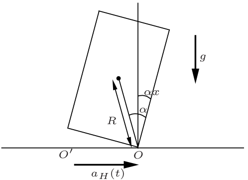
Figure 7: Rocking block

This system was first studied in [Hou63]. The equations that govern its behaviour are well known (see for example [YCP80, SK84]), and are given by

$$\alpha\ddot{x}+\text{sign}(x)\sin(\alpha(1 -\text{sign}\left(x\right)x))=$$

$$-\alpha\varepsilon\cos\left(\alpha\left(1-\text{sign}\left(x\right)x\right)\right)\cos\left(\omega t\right)$$ (5.2)

$$\dot{x}(t^{+}_{A})=r\dot{x}(t^{-}_{A})\hskip 14.22636pt(x=0)$$ (5.3)

where the last equation, (5.3), simulates the loss of energy of the block at every impact with the ground, as described in §2.3. In addition, the function

$$\text{sign}(x)=\left\{\begin{aligned} 1&&\text{if }x>0\\ -1&&\text{if }x<0\end{aligned}\right.$$ (5.4)

distinguishes between the two modes of movement: rocking about the point $O$ when the angle is positive ($x>0$) or rocking about $O^{\prime}$ when the angle $x$ is negative. Obviously, this makes the system piecewise smooth and so it can be written in the form of Eq. (2.2). Moreover, conditions C.1–C.5  are satisfied and, hence, the results shown in previous sections can be applied. However, as our purpose here is to illustrate them, we will consider the linearized version of Eq. (5.2) instead, which will permit us to perform explicit analytical computations. This linearization is achieved by assuming $\alpha\ll 1$, namely that the block is slender [Hog89]. Thus, the system that we will consider, written in the form of Eq. (2.2), is

$$\left.\begin{aligned} \dot{x}=&y\\ \dot{y}=&x-1-\varepsilon\cos\left(\omega t\right)\end{aligned}\right\} \text{ if }x>0$$ (5.5)

$$\left.\begin{aligned} \dot{x}=&y\\ \dot{y}=&x+1-\varepsilon\cos\left(\omega t\right)\end{aligned}\right\} \text{ if }x<0$$ (5.6)

$$y(t^{+}_{A})=ry(t^{-}_{A}) \hskip 14.22636pt(x=0),$$ (5.7)

where the perturbation becomes a smooth function due to the linearization.
If $r=1$, system (5.5)-(5.6) can be written in the form (2.5) using the Hamiltonian function

$$H_{\varepsilon}(x,y,t)=H_{0}(x,y)+\varepsilon H_{1}(x,t),$$ (5.8)

where

$$H_{0}(x,y)=\left\{\begin{aligned} \frac{y^{2}}{2}-\frac{x^{2}}{2}+x,&\text{ if }x>0\\ \frac{y^{2}}{2}-\frac{x^{2}}{2}-x,&\text{ if }x<0\end{aligned}\right.$$ (5.9)

and

$$H_{1}(x,t)=x\cos\left(\omega t\right)$$ (5.10)

is $T$-periodic, with $T=2\pi/\omega$ and is a $C^{\infty}$ function.
In addition, when $\varepsilon=0$, conditions C.1–C.5 are fulfilled, and the phase portrait for the system (5.5)-(5.6) is equivalent to the one shown in Fig. 1. That is, it possesses an invisible fold-fold of centre type at the origin and two saddle points at $(1,0)$ and $(-1,0)$ connected by two heteroclinic orbits. Furthermore, the origin is surrounded by a continuum of periodic orbits whose periods monotonically increase as they approach to the heteroclinic connections. Using Eqs. (2.15) and (2.16), the symmetries of the Hamiltonian (5.9) and assuming $y_{0}>0$, these periods are given by

$$\alpha(y_{0}) =4\int_{0}^{1-\sqrt{1-y_{0}^{2}}}\frac{1}{\sqrt{y_{0}^{2}+x^{2}-2x}}dx=$$

$$=2\ln\left(\frac{1+y_{0}}{1-y_{0}}\right),$$ (5.11)

and hence $\alpha^{\prime}(y_{0})>0$.

5.2 Existence of periodic orbits

We first study the persistence of $(n,m)$-periodic orbits for $r=1$ in Eq. (5.7) by applying Theorem 1. The subharmonic Melnikov function (3.3) becomes

$$M^{n,m}(t_{0})=-\int_{0}^{nT}\Pi_{y}(q_{c}(t))\cos(\omega\left(t+t_{0}\right))dt,$$ (5.12)

where $q_{c}(t)$ is the periodic orbit of the unperturbed version of system (5.5)-(5.6) with Hamiltonian $c=\frac{\bar{y}_{0}^{2}}{2}$ satisfying $q_{c}(0)=(0,\bar{y}_{0})$ and

$$\bar{y}_{0}=\alpha^{-1}\left(\frac{nT}{m}\right)=\frac{e^{\frac{nT}{2m}}-1}{e^{\frac{nT}{2m}}+1}.$$ (5.13)

We now want to obtain an explicit expression for Eq. (5.12). Thus we first note that the solution of system (5.5)-(5.6) with initial condition $(x_{0},y_{0})$ at $t=t_{0}$ is given by

$$x^{\pm}(t) =C_{1}^{\pm}e^{t}+C_{2}^{\pm}e^{-t}\pm 1$$ (5.14)

$$y^{\pm}(t) =C_{1}^{\pm}e^{t}-C_{2}^{\pm}e^{-t},$$ (5.15)

where

$$C_{1}^{\pm}=\frac{x_{0}+y_{0}\mp 1}{2}e^{-t_{0}},\;C_{2}^{\pm}=\frac{x_{0}-y_{0}\mp 1}{2}e^{t_{0}}.$$ (5.16)

As explained in §2.4, the superscript $+$ is applied if $x_{0}>0$ or $x_{0}=0$ and $y_{0}>0$, and the $-$ otherwise.
Assuming $x_{0}=0$ and $y_{0}=\bar{y}_{0}>0$, an expression for $\Pi_{y}(q_{c}(t))$ becomes

$$\Pi_{y}(q_{c}(t))=\left\{\begin{aligned} C_{1}e^{t}-C_{2}e^{-t},&&&\text{ if }0\leq t\leq\frac{nT}{2m}\\ -C_{1}e^{t-\frac{nT}{2m}}+C_{2}e^{-t+\frac{nT}{2m}},&&&\text{ if }\frac{nT}{2m}\leq t\leq\frac{nT}{m},\end{aligned}\right.$$ (5.17)

where

$$C_{1}=\frac{\bar{y}_{0}-1}{2},\;C_{2}=\frac{-\bar{y}_{0}-1}{2}.$$ (5.18)

Thus, Eq. (5.12) becomes

$$M^{n,m}(t_{0})=-\sum_{j=0}^{m-1}\Bigg{(}\int_{0}^{\frac{nT}{2m}}\left(C_{1}e^{t}-C_{2}e^{-t}\right)\cos\left(\omega\left(t+t_{0}+j\frac{nT}{m}\right)\right)dt$$

$$+\int_{\frac{nT}{2m}}^{\frac{nT}{m}}\left(-C_{1}e^{t-\frac{nT}{2m}}+C_{2}e^{-t+\frac{nT}{2m}}\right)\cos\left(\omega\left(t+t_{0}+j\frac{nT}{m}\right)\right)dt\Bigg{)}$$

and, after some computations, we have

$$M^{n,m}(t_{0})=\left\{\begin{aligned} -\frac{4}{\omega^{2}+1}\cos\left(\omega t_{0}\right),&&&\text{ if }m=1\\ 0,&&&\text{ if }m>1.\end{aligned}\right.$$ (5.19)

As $M^{n,1}(t_{0})$ has two simple zeros, $\bar{t}_{0}^{1}=\frac{T}{4}$ and $\bar{t}_{0}^{2}=\frac{3T}{4}$, by Theorem 1, if $\varepsilon>0$ is small enough, the non-autonomous system (5.5)-(5.6) possesses two subharmonic $(n,1)$-periodic orbits. In addition, the initial conditions of these periodic orbits are $\varepsilon$-close to

$$(0,\bar{y}_{0},\bar{t}_{0}^{1})=(0,\frac{e^{\frac{nT}{2}}-1}{e^{\frac{nT}{2}}+1},\frac{T}{4})$$ (5.20)

and

$$(0,\bar{y}_{0},\bar{t}_{0}^{2})=(0,\frac{e^{\frac{nT}{2}}-1}{e^{\frac{nT}{2}}+1},\frac{3T}{4}),$$ (5.21)

respectively.
Proceeding as in Remark 3, one can solve numerically Eq. (3.2) with $m=1$ and find the initial conditions for such a periodic orbit. In Fig. 8 we show the result of that for $n=5$. Each periodic orbit is obtained by using the points given in Eqs. (5.20) and (5.21) to initiate the Newton method. Then, tracking the obtained solution, $\varepsilon$ has been increased up to $\varepsilon=1.6565\cdot 10^{-2}$.

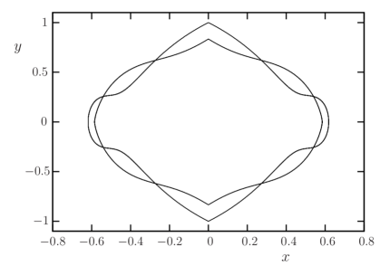
Figure 8: Periodic orbits for $n=5$ and $m=1$, $\omega=5$ and $\varepsilon=1.6565\cdot 10^{-2}$. Their initial conditions are $\varepsilon$-close to the points given in Eqs. (5.20) and (5.21).

Regarding the existence of $(n,m)$-periodic orbits with $m>1$ (ultrasubharmonic orbits), as the subharmonic Melnikov function is identically zero nothing can be said using the first order analysis that we have shown in this work.
However, if instead (5.10) one considers the perturbation

$$H_{1}(x,t)=x\left(\cos\left(\omega t\right)+\cos\left(k\omega t\right)\right),$$

then, it can be seen that the corresponding Melnikov function possesses simple zeros for $m=k$ and $n$ relatively prime odd integers. Thus, periodic orbits impacting $m>1$ times with the switching manifold can exist if higher harmonics of the perturbation are considered.

Let us now introduce the energy dissipation described in §3.2 and consider the whole system (5.5)-(5.7) with $r<1$ using the Hamiltonian perturbation (5.8). From Theorem 2, simple zeros of the Melnikov function (5.19) also guarantee the existence of $(n,1)$-periodic orbits when $1-r$ is small enough with respect to $\varepsilon$. More precisely, taking

$$\varepsilon=\tilde{\varepsilon}\delta,\;r=1-\tilde{r}\delta,$$ (5.22)

condition (3.18) becomes

$$0<\frac{\tilde{r}}{\tilde{\varepsilon}}<\frac{1}{2}\left(\frac{e^{\frac{nT}{2}}+1}{e^{\frac{nT}{2}}-1}\right)^{2}M^{n,1}(t_{M}):=\rho,$$ (5.23)

where $M^{n,1}(t_{M})=M^{n,1}(\frac{T}{2})=\frac{4}{\omega^{2}+1}$ is the maximum value of the Melnikov function (5.19). Then there exists an $(n,1)$-periodic orbit if $\delta>0$ is small enough. The initial condition of the periodic orbit is located in a $\delta$-neighbourhood of the point $(x_{0},y_{0},t_{0})=(0,\bar{y}_{0},\widehat{t}_{0})$, where $\bar{y}_{0}$ is defined in Eq. (5.13), such that

$$\alpha(\bar{y}_{0})=nT$$

and $\widehat{t}_{0}$ is given by the simple zeros of Eq. (3.17), which becomes

$$-2\tilde{r}\bar{y}_{0}^{2}+\tilde{\varepsilon}M^{n,1}(t_{0})=0.$$ (5.24)

Hence we find

$$\widehat{t}_{0}^{i}=\frac{1}{\omega}\arccos\left(-\frac{\omega^{2}+1}{2}\left(\frac{e^{\frac{nT}{2}}-1}{e^{\frac{nT}{2}}+1}\right)^{2}\frac{\tilde{r}}{\tilde{\varepsilon}}\right)+(i-1)\frac{T}{2},\;i=1,2.$$ (5.25)

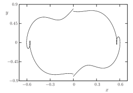
(a) $\delta=1.04$

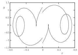
(b) $\delta=4.125$

Figure 9: $(5,1)$-periodic orbits for $\omega=5$ and $\frac{\tilde{r}}{\tilde{\varepsilon}}=0.07$. Tracking the obtained solution, the perturbation parameter $\delta$ has been increased up to its maximum value. Initial conditions close to $(\bar{y}_{0},\widehat{t}_{0}^{1})$ and $(\bar{y}_{0},\widehat{t}_{0}^{2})$ have been used in (a) and (b), respectively.

As before, we set $n=5$ and $\omega=5$. Then expression (5.23) becomes

$$0<\frac{\tilde{r}}{\tilde{\varepsilon}}<0.0914.$$ (5.26)

Hence, for any fixed ratio $\frac{\tilde{r}}{\tilde{\varepsilon}}$ satisfying (5.26) there exist two points, $(\bar{y}_{0},\widehat{t}_{0}^{i})$, $i=1,2$, such that, if $\delta$ is small enough, Eq. (3.10) possesses a solution $\delta$-close to them. Such a solution is an initial condition for an $(n,1)$-periodic orbit of system (5.5)-(5.7), with $r=1-\tilde{r}\delta$ and $\varepsilon=\tilde{\varepsilon}\delta$.

In Fig. 9 some of these orbits are shown for one value of the ratio satisfying (5.26). Two different periodic orbits are shown, which are the ones whose initial conditions are $\delta$-close to the values $(\bar{y}_{0},\widehat{t}_{0}^{1})$ and $(\bar{y}_{0},\widehat{t}_{0}^{2})$. In both cases, $\delta$ tracks the solution, up to the value from which solutions of Eq. (5.23) can no longer be found. These are the values used in the simulations shown in Fig. 9. Above the limiting value of the ratio given in (5.26), no $(5,1)$-periodic orbits were found for $\omega=5$.

5.3 Existence curves

We now use Theorem 2 to derive existence curves for the $(n,1)$-periodic orbits ($n$ odd) and compare them with the ones obtained in [Hog89]. Unlike in [Hog89], we obtain these curves in the $r$-$\varepsilon$ plane through the variation of $\delta$.
The limiting condition provided by Theorem 2 is given in Eq. (5.23). Thus, for a given $r$ close to $1$ ($\tilde{r}\delta$ close to 0), it is natural to arbitrarily fix $\tilde{r}$ and minimize $\varepsilon$ by maximizing the ratio in (5.23), setting $\frac{\tilde{r}}{\tilde{\varepsilon}}=\rho$. However, the upper boundary of $\delta$, $\delta_{0}$, provided by Theorem 2 tends to zero as $\frac{\tilde{r}}{\tilde{\varepsilon}}\to\rho$, as it is derived from the implicit function theorem. Thus, it is not possible to uniformally bound $\delta$ for all the ratios between $0$ and $\rho$. Hence, the condition $\frac{\tilde{r}}{\tilde{\varepsilon}}=\rho$ can not be used to derive a limiting relation between $r$ and $\varepsilon$. Instead, we proceed as follows.
We first fix $n$ odd and $\omega>0$. Then, for every ratio $0<\frac{\tilde{r}}{\tilde{\varepsilon}}<\rho$, we increase $\delta$ from $0$ to $\delta_{0}$ by numerically tracking the obtained solution using as initial seed one of the values provided in Eq. (5.20) or (5.21). This results in a curve in the $r$-$\varepsilon$ plane parametrized by the ratio $\frac{\tilde{r}}{\tilde{\varepsilon}}$.
Regarding the results obtained in [Hog89], such a curve was obtained analytically and for global conditions, and has the expression

$$\varepsilon_{\text{min}}(R)=\frac{\left(1+\omega^{2}\right)R\left(1-\cosh\left(\frac{nT}{2}\right)\right)}{\sqrt{\omega^{2}\sinh^{2}\left(\frac{nT}{2}\right)R^{2}+\left(2-R\right)^{2}\left(1+\cosh\left(\frac{nT}{2}\right)\right)^{2}}},$$ (5.27)

where $R=1-r$.
As our result is only locally valid, in order to compare both results we have to check whether both curves are tangent at $\varepsilon=0$. From (5.27) we easily obtain

$$\varepsilon_{\text{min}}^{\prime}(0)=-\frac{1+\omega^{2}}{2}\left(\frac{e^{\frac{nT}{2}}-1}{e^{\frac{nT}{2}}+1}\right)^{2}=-\frac{1}{\rho},$$

which, by the inverse function theorem, tells us that both curves are tangent at $\varepsilon=0$.

In Fig. 10, we show an example for $n=5$ and $\omega=5$ using initial conditions near (5.20). As can be seen, the curve provides, for every value of $r$, both the maximum and minimum values of $\varepsilon$ for which a $(5,1)$-periodic orbit exists. The lower boundary derived in [Hog89], $\left(\varepsilon_{\text{min}}(\cdot)\right)\!^{-1}\!(\varepsilon)$ is also shown. As demonstrated above, both curves are tangent at $\varepsilon=0$, with slope equal to $\rho$. Note that the lower boundary does not coincide with the line $1-r=\rho\varepsilon$, although their difference tends to zero as $r\to 1$. This confirms that one can not derive the minimum value of $\varepsilon$ from condition (5.23) for every fixed $r$.

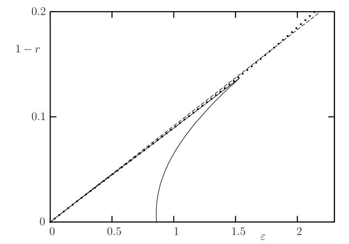
Figure 10: Existence curves of a $(5,1)$-periodic orbit for $\omega=5$. Expression derived from Theorem 2 (black line), expression for $\varepsilon_{\text{min}}$ derived from [Hog89] (dotted curve) and line $1-r=\rho\varepsilon$ (dashed).

References

- [BF08] Flaviano Battelli and Michal Fečkan. Homoclinic trajectories in discontinuous systems. Journal of Dynamics and Differential Equations, 20:337–376, 2008. 10.1007/s10884-007-9087-9.
- [BK91] B. Bruhn and B. P. Koch. Heteroclinic bifurcations and invariant manifolds in rocking block dynamics. Z. Naturforsch., 46a:481–490, 1991.
- [GH83] J. Guckenheimer and P. J. Holmes. Nonlinear Oscillations, Dynamical Systems and Bifurcations of Vector Fields. Applied Mathematical Sciences. Springer, 4 edition, 1983.
- [GST11] M. Guardia, T. M. Seara, and M. A. Teixeira. Generic bifurcations of low codimension of planar Filippov Systems. Journal of Differential Equations, 250:1967–2023, 2011.
- [Hog89] S. J. Hogan. On the dynamiccs of rigid block motion under harmonic forcing. Proc. Royal Society of London A, 425:441–476, 1989.
- [Hog92] S. J. Hogan. Heteroclinic bifurcations in damped rigid block motion. Proc. Royal Society of London A, 439:155–162, 1992.
- [Hou63] G.W. Housner. The behaviour of inverted pendulum structures during earthquakes. Bull. seism. Soc. Am., 53:403–417, 1963.
- [KKY97] M. Kunze, T. Küpper, and J. You. On the application of KAM theory to discontinuous dynamical systems. Journal of Differential Equations, 139:1–21, 1997.
- [Kuk07] P. Kukučka. Melnikov method for discontinuous planar systems. Nonlinear Analysis, 66:2698–2719, 2007.
- [Kun00] M. Kunze. Non-Smooth Dynamical Systems. Springer-Verlag, 2000.
- [SK84] P. D. Spanos and A.-S. Koh. Rocking of rigid blocks due to harmonic shaking. J. eng. Mech. Div. Am. Soc. Civ. Engrs., 110:1627–1642, 1984.
- [YCP80] C.-S. Yim, A. K. Chopra, and J. Penzien. Rocking response of rigid blocks to earthquakes. Earthquake Engng. struct. Dyn., 8:565–587, 1980.