New initial condition of the new agegraphic dark energy model

Abstract

The initial condition $\Omega_{\rm de}(z_{\rm ini})=n^{2}(1+z_{\rm ini})^{-2}/4$ at $z_{\rm ini}=2000$ widely used to solve the differential equation of the density of the new agegraphic dark energy (NADE) $\Omega_{\rm de}$, makes the NADE model be a single-parameter dark-energy cosmological model. However, we find that this initial condition is only applicable in a flat universe with only dark energy and pressureless matter. In fact, in order to obtain more information from current observational data, such as cosmic microwave background (CMB) and baryon acoustic oscillations (BAO), we need to consider the contribution of radiation. For this situation, the initial condition mentioned above becomes invalid. To overcome this shortage, we investigate the evolution of dark energy in the matter-dominated and radiation-dominated epochs, and obtain a new initial condition $\Omega_{\rm de}(z_{\rm ini})=\frac{n^{2}(1+z_{\rm ini})^{-2}}{4}\left(1+\sqrt{F(z_{\rm ini})}\right)^{2}$ at $z_{\rm ini}=2000$, where $F(z)\equiv\frac{\Omega_{r0}(1+z)}{\Omega_{m0}+\Omega_{r0}(1+z)}$ with $\Omega_{r0}$ and $\Omega_{m0}$ being the current density parameters of radiation and pressureless matter, respectively. This revised initial condition is applicable for the differential equation of $\Omega_{\rm de}$ obtained in the standard Friedmann-Robertson-Walker (FRW) universe with dark energy, pressureless matter, radiation, and even spatial curvature, and can still keep the NADE model being a single-parameter model. With the revised initial condition and the observational data of type Ia supernova (SNIa), CMB and BAO, we finally constrain the NADE model. The results show that the single free parameter $n$ of the NADE model can be constrained tightly.

I Introduction

The accelerated expansion of current universe, first observed in 1998 [1], implies that our universe is being dominated by an exotic component with negative pressure dubbed dark energy. To understand its nature, we should first ascertain its dynamic evolution. For many dark energy models, it is believed that the models are favored by observations if they can fit the data well with less free parameters, since the less parameters may be constrained tightly. To our knowledge, in dark-energy cosmology, there exist three rare dark energy models, namely, the Lambda Cold Dark Matter ($\Lambda$CDM) [2], the Dvali-Gabadadze-Porrati (DGP) braneworld [3], and the new agegraphic dark energy (NADE) [4] models, which contain only one free model parameter. Among these three models, the NADE model is a special one, because unlike the other two models whose single-parameter feature is obvious, the NADE model is due to its special analytic feature in the matter-dominated epoch [5]. To see it clearly, we first briefly review the NADE model.

The dark energy density $\rho_{\rm de}$ in the NADE model, constructed in light of the Károlyházy relation [6] and corresponding energy fluctuations of space-time, has the form [4]

$$\rho_{\rm de}=\frac{3n^{2}M_{\rm Pl}^{2}}{\eta^{2}},$$ (1)

where $n$ is a numerical parameter, $M_{\rm Pl}$ is the reduced Planck mass. The $\eta$ is the conformal age of the universe

$$\eta\equiv\int_{0}^{t}\frac{dt^{\prime}}{a}=\int_{0}^{a}\frac{da^{\prime}}{Ha^{\prime 2}},$$ (2)

where $a$ is the scale factor of the universe, and $H\equiv\dot{a}/a$ is the Hubble parameter. Here the overdot denotes the derivative with respect to the cosmic time $t$. In a flat universe containing dark energy and pressureless matter, the Friedmann equation can be written as $\Omega_{\rm de}+\Omega_{m}=1$, where $\Omega_{\rm de}$ and $\Omega_{m}$ are defined as the ratio of the densities of dark energy $\rho_{\rm de}$ and matter $\rho_{m}$ to the critical density $\rho_{\rm crit}\equiv{3M_{\rm Pl}^{2}H^{2}}$, respectively. From the Friedmann equation, Eqs. (1) and (2), and the energy conservation equation $\dot{\rho}_{m}+3H\rho_{m}=0$, we can derive a differential equation of $\Omega_{\rm de}(z)$ [4]

$$\frac{d\Omega_{\rm de}}{dz}=-\frac{\Omega_{\rm de}}{1+z}\left(1-\Omega_{\rm de}\right)\left[3-\frac{2\left(1+z\right)}{n}\sqrt{\Omega_{\rm de}}\right],$$ (3)

where $z=a^{-1}-1$ is redshift. Furthermore, combining Eqs. (1) and (2) with the energy conservation equation $\dot{\rho}_{\rm de}+3H(1+w)\rho_{\rm de}=0$, we can easily find that the equation-of-state parameter (EOS) of NADE is given by [4]

$$w=-1+\frac{2}{3n}\frac{\sqrt{\Omega_{\rm de}}}{a}.$$ (4)

At the first glance, one might consider that NADE is a two-parameter model, since besides parameter $n$ the model has another free parameter $\Omega_{m0}$ coming from the natural initial condition $\Omega_{\rm de0}=1-\Omega_{m0}$ in solving Eq. (3) (note that the subscript “0” denotes the present value of the corresponding quantity, hereafter). However, as shown in Ref. [5], the NADE model is actually a single-parameter model in practice, thanks to its special analytic feature $\Omega_{\rm de}=n^{2}a^{2}/4$ in the matter-dominated epoch. To obtain this relation, we can consider the matter-dominated epoch, in which $H^{2}\propto\rho_{m}\propto{a^{-3}}$. From Eqs. (1) and (2), we obtain $\rho_{\rm de}\propto{a^{-1}}$. Then, from the energy conservation equation $\dot{\rho}_{\rm de}+3H(1+w)\rho_{\rm de}=0$, we have $w=-2/3$. Comparing $w=-2/3$ with Eq. (4), we find that $\Omega_{\rm de}=n^{2}a^{2}/4=n^{2}(1+z)^{-2}/4$. Note that this relation is also one of the analytic solutions of

$$\frac{d\Omega_{\rm de}}{dz}=\frac{-\Omega_{\rm de}}{1+z}\left[3-\frac{2(1+z)}{n}\sqrt{\Omega_{\rm de}}\right],$$ (5)

which is the reduced form of Eq. (3), since $1-\Omega_{\rm de}\simeq 1$ in the matter-dominated epoch. Thus, once the value of $n$ is given, Eq. (3) can be numerically solved by using $\Omega_{\rm de}(z_{\rm ini})=n^{2}(1+z_{\rm ini})^{-2}/4$ at any $z_{\rm ini}$ deep into the matter-dominated epoch ($z_{\rm ini}=2000$ is chosen in Ref. [5]).

By using the initial condition $\Omega_{\rm de}(z_{\rm ini})=n^{2}(1+z_{\rm ini})^{-2}/4$ at $z_{\rm ini}=2000$ and the observational data, Wei and Cai [5] firstly constrained the single-parameter NADE model. After their work, this initial condition was widely used in the literature; see, e.g., Refs. [7, 8, 9]. All results showed that the only free parameter $n$ could be constrained tightly and the NADE model could fit the observational data well.

However, the fly in the ointment is that the initial condition $\Omega_{\rm de}(z_{\rm ini})=n^{2}(1+z_{\rm ini})^{-2}/4$ at $z_{\rm ini}=2000$ is obtained by considering a flat universe containing only dark energy and pressureless matter. So, a natural question we may ask is whether this initial condition is applicable when we consider the contribution from radiation. Before we answer this question, let us first see why we need this discussion.

We all know that the cosmic microwave background (CMB) and large-scale structure (LSS) observations play an essential role in testing the cosmological model and constraining its basic parameters. Generally, we might need to use the full data of CMB (CMB temperature and polarization power spectra) and LSS (matter power spectrum) to perform a global fitting. However, such a fitting consumes a large amount of time and power. As an alternative, two methods are widely utilized: (i) using the shift parameter $R$ from CMB [10, 11] and distance parameter $A$ of the BAO measurement [12], (ii) employing the distance prior including $R$, $l_{A}$ and $z_{*}$ from CMB [13] and $r_{s}(z_{d})/D_{V}(z)$ from BAO measurement of Sloan Digital Sky Survey (SDSS) [14]. Here $r_{s}(z)$ is the comoving sound horizon whose fitting formula is given by

$$r_{s}(z)=\frac{1}{\sqrt{3}}\int_{0}^{1/(1+z)}\frac{da}{a^{2}H(a)\sqrt{1+(3\Omega_{b0}/4\Omega_{\gamma 0})a}},$$ (6)

where the present photon density parameter $\Omega_{\gamma 0}=2.469\times 10^{-5}h^{-2}$ (for $T_{\rm cmb}=2.725$ K) with $h$ the Hubble constant $H_{0}$ in units of 100 km s^-1 Mpc^-1, and $\Omega_{b0}$ is the present baryon density parameter. For the other quantities mentioned in the method (ii), we will illustrate them in detail in Sec. III. There is no doubt that the method (ii) encodes more information of the CMB and LSS data. Note that the distance prior ($R$, $l_{A}$, $z_{*}$), as shown in Ref. [13], is applicable only when the model in question is based on the standard Friedmann-Robertson-Walker (FRW) universe with pressureless matter, radiation, dark energy, and spatial curvature. Since the integral in Eq. (6) involves the early radiation-dominated epoch, we need to consider the contribution of radiation when utilizing $r_{s}(z_{d})/D_{V}(z)$ of the BAO measurement. To sum up, in order to use the method (ii), we need to consider the contribution of radiation besides the pressureless matter and dark energy.

In the following, we will show that the initial condition $\Omega_{\rm de}(z_{\rm ini})=n^{2}(1+z_{\rm ini})^{-2}/4$ at $z_{\rm ini}=2000$ needs to be amended to accommodate method (ii) in using the CMB and BAO data. Then, with the revised initial condition and the current observational data including type Ia supernovae (SNIa), CMB and BAO, we will constrain the NADE model in a flat universe with dark energy, matter, and radiation.

II New initial condition

In a flat universe with dark energy, matter, and radiation, the Friedmann equation reads

$$\Omega_{\rm de}+\Omega_{m}+\Omega_{r}=1,$$ (7)

where $\Omega_{r}$ is the ratio of the energy density of radiation $\rho_{r}$ to the critical density $\rho_{\rm crit}$. Using Eqs. (1), (2), and (7), and combining the energy conservation equations $\dot{\rho}_{m}+3H\rho_{m}=0$ and $\dot{\rho}_{r}+4H\rho_{r}=0$, we can easily derive the differential equation of $\Omega_{\rm de}(z)$,

$$\frac{d\Omega_{\rm de}}{dz}=\frac{-\Omega_{\rm de}}{1+z}\left(1-\Omega_{\rm de}\right)\left[3+F(z)-\frac{2(1+z)}{n}\sqrt{\Omega_{\rm de}}\right],$$ (8)

where $F(z)\equiv\frac{\Omega_{r0}(1+z)}{\Omega_{m0}+\Omega_{r0}(1+z)}$.

To solve Eq. (8), of course, we may use the initial condition $\Omega_{\rm de0}=1-\Omega_{m0}-\Omega_{r0}$. However, such a treatment will add an extra parameter $\Omega_{m0}$ to the NADE model, as mentioned above (note that one usually fixes $\Omega_{r0}=\Omega_{\gamma 0}(1+0.2271N_{\rm eff})$, and the standard value 3.04 of the effective number of neutrino species $N_{\rm eff}$ is required [13]). Moreover, it has been shown in Ref. [9] that such a two-parameter NADE model cannot be constrained well by observational data (e.g., $137.702<n<337.974$ at the $1\sigma$ level). On the other hand, if we expect that $\Omega_{\rm de}(z_{\rm ini})=n^{2}(1+z_{\rm ini})^{-2}/4$ at $z_{\rm ini}=2000$ is able to be used as the initial condition in solving Eq. (8), we must require it at least to satisfy the equation

$$\frac{d\Omega_{\rm de}}{dz}=\frac{-\Omega_{\rm de}}{1+z}\left[3+F(z)-\frac{2(1+z)}{n}\sqrt{\Omega_{\rm de}}\right],$$ (9)

which is the reduced form of Eq. (8). Here $1-\Omega_{\rm de}\simeq 1$ in the matter-dominated epoch is used. Comparing Eq. (9) with Eq. (5), we can find that the above condition depends on $F(z)\ll 1$ in the matter-dominated epoch, since $\Omega_{\rm de}=n^{2}(1+z)^{-2}/4$ satisfies Eq. (5) accurately. However, from the definition $F(z)\equiv\frac{\Omega_{r0}(1+z)}{\Omega_{m0}+\Omega_{r0}(1+z)}$, it may have a visible value because of $z\gg 1$ in the matter-dominated epoch, even though $\Omega_{r0}\ll\Omega_{m0}$. In fact, we can check that $F(2000)=0.3850$ if we choose $\Omega_{m0}=0.1334\times{h^{-2}}$ according to the recent WMAP observations [13]. Thus the existence of the non-ignorable $F(z)$ indicates that we need to find a new initial condition to solve Eq. (8).

Fortunately, it is not that hard to obtain the new initial condition applicable for Eq. (8). Let us consider an epoch when the density of dark energy can be ignored; but we do not need to distinguish the matter-dominated or the radiation-dominated epoch; then we have $H^{2}\propto\Omega_{m0}a^{-3}+\Omega_{r0}a^{-4}$. From the definition of the conformal age of the universe, we have $\eta\propto\sqrt{\Omega_{m0}a+\Omega_{r0}}-\sqrt{\Omega_{r0}}.$ Then, from Eq. (1), we can obtain

$$\rho_{\rm de}\propto\left(\sqrt{\Omega_{m0}a+\Omega_{r0}}-\sqrt{\Omega_{r0}}\right)^{-2}.$$ (10)

Combining Eq. (10) with the energy conservation equation $\dot{\rho}_{\rm de}+3H(1+w)\rho_{\rm de}=0$, we can obtain the EOS of dark energy at this epoch,

$$w=-\frac{2}{3}+\frac{1}{3}\sqrt{\frac{\Omega_{r0}}{\Omega_{m0}a+\Omega_{r0}}}.$$ (11)

Then, comparing Eq. (11) with Eq. (4), we can easily obtain

$$\Omega_{\rm de}=\frac{n^{2}(1+z)^{-2}}{4}\left(1+\sqrt{F(z)}\right)^{2}.$$ (12)

Furthermore, one can also check that Eq. (12) is an analytic solution of Eq. (9). As the evolution of $\Omega_{\rm de}$ satisfies Eq. (12) both in the matter-dominated and the radiation-dominated epochs, we can use Eq. (12) at any $z_{\rm ini}$ in these two epochs as the initial condition to solve Eq. (8) numerically. In our work, we follow Ref. [5] and still choose $z_{\rm ini}=2000$. Then, a new initial condition $\Omega_{\rm de}(z_{\rm ini})=\frac{n^{2}(1+z_{\rm ini})^{-2}}{4}\left(1+\sqrt{F(z_{\rm ini})}\right)^{2}$ at $z_{\rm ini}=2000$ is available for the NADE model in a flat universe with dark energy, pressureless matter, and radiation. In fact, this new initial condition is also valid in a non-flat universe, since the spatial curvature $\Omega_{k}$ is much smaller than $\Omega_{m}$ or $\Omega_{r}$ at $z=2000$. It is interesting to make a comparison between the new initial condition and the old one $\Omega_{\rm de}(z_{\rm ini})=n^{2}(1+z_{\rm ini})^{-2}/4$ at $z_{\rm ini}=2000$. Obviously, their difference comes from the term $\left(1+\sqrt{F(z_{\rm ini})}\right)^{2}$ whose value is 2.626 at $z_{\rm ini}=2000$, which means that the density of dark energy at $z=2000$ given by the new initial condition is about 2.6 times larger than that given by the original initial condition.

Up to now, we have discussed the new initial condition theoretically. Next, we test the new initial condition by using the observational data to constrain the NADE model with the new initial condition. To achieve this, we will use a Markov chain Monte-Carlo (MCMC) method. However, before doing this, we still need to overcome a technical difficulty. It is well known that we need to give initial free parameters to launch the MCMC. For our work, as our purpose of finding the new initial condition is to keep the single-parameter feature of the NADE model, we only give an initial value of the single free parameter $n$. Here, the difficulty is how to numerically solve Eq. (8) using the new initial condition $\Omega_{\rm de}(z_{\rm ini})=\frac{n^{2}(1+z_{\rm ini})^{-2}}{4}\left(1+\sqrt{F(z_{\rm ini})}\right)^{2}$ at $z_{\rm ini}=2000$, as we only know the initial value of $n$ but have no idea about $\Omega_{m0}$ (the value of $\Omega_{r0}$ is fixed as mentioned above). Note that both Eq. (8) and the new initial condition explicitly contain parameter $\Omega_{m0}$.

For this problem, actually we have many methods. Here, we introduce two methods. The first one is treating the non-independent parameter $\Omega_{m0}$ as a variable. Thus, Eq. (8) becomes a partial differential equation,

$$\frac{\partial\ln\Omega_{\rm de}}{\partial{z}}=\frac{\Omega_{\rm de}-1}{1+z}\left[3+\frac{\Omega_{r0}(1+z)}{\Omega_{m0}+\Omega_{r0}(1+z)}-\frac{2(1+z)}{n}\sqrt{\Omega_{\rm de}}\right],$$ (13)

where $\Omega_{\rm de}=\Omega_{\rm de}(z,~{}\Omega_{m0})$ is a function of the two variables $z$ and $\Omega_{m0}$. Thus, giving a value of $n$ and a range of $\Omega_{m0}$, we can numerically solve the partial differential equation (13) by using the new initial condition $\Omega_{\rm de}(z_{\rm ini},~{}\Omega_{m0})=\frac{n^{2}(1+z_{\rm ini})^{-2}}{4}\left(1+\sqrt{F(z_{\rm ini},~{}\Omega_{m0})}\right)^{2}$ at $z_{\rm ini}=2000$. Then, with the result of $\Omega_{\rm de}(z,~{}\Omega_{m0})$, we can obtain the value of $\Omega_{m0}$ by numerically finding the root of the equation $\Omega_{\rm de}(0,~{}\Omega_{m0})=1-\Omega_{m0}-\Omega_{r0}$. Substituting $\Omega_{m0}$ back into $\Omega_{\rm de}(z,~{}\Omega_{m0})$, we can obtain the evolution of $\Omega_{\rm de}(z)$.

We can also use a numerical iterative method, namely, generating a sequence $\{\Omega_{m0}^{(i)}\}$ by the iterative formula $\Omega_{m0}^{(l+1)}=1-\Omega_{\rm de}(0)|_{\Omega_{m0}^{(l)}}-\Omega_{r0}$. Here, $\Omega_{\rm de}(z)|_{\Omega_{m0}^{(l)}}$ is the numerical solution of Eq. (8) with $\Omega_{m0}=\Omega_{m0}^{(l)}$. Thus, for the current value of $\Omega_{m0}^{(l)}$, a new value $\Omega_{m0}^{(l+1)}$ can be obtained from the iterative formula. We can choose the initial value $\Omega_{m0}^{(0)}=0.27$ and set a termination condition for the iteration, such as $\left|\Omega_{m0}^{(l+1)}-\Omega_{m0}^{(l)}\right|\leq{\epsilon}$ with $\epsilon$ a small quantity. Our practice shows that its convergence speed is very fast, and generally, the number of the iteration is less than 5 for $\epsilon=10^{-6}$.

Using the two methods mentioned above, we find the evolution of $\Omega_{\rm de}(z)$ for a given value of the single free parameter $n$. Then, the dimensionless Hubble expansion rate is given by

$$E(z)\equiv{H(z)\over H_{0}}=\left[\frac{\Omega_{m0}(1+z)^{3}+\Omega_{r0}(1+z)^{4}}{1-\Omega_{\rm de}(z)}\right]^{1/2}.$$ (14)

III Observational data and results

In this section, we constrain the NADE model with the new initial condition by using the data from Union2 SNIa (557 data) [15] and observations of CMB from 7-year WMAP [13] and BAO from SDSS DR7 [14].

The data of the 557 Union2 SNIa are compiled in Ref. [15]. The theoretical distance modulus is defined as

$$\mu_{\rm th}(z_{i})\equiv 5\log_{10}D_{L}(z_{i})+\mu_{0},$$ (15)

where $\mu_{0}\equiv 42.38-5\log_{10}h$ and the Hubble-free luminosity distance is

$$D_{L}(z)=(1+z)\int_{0}^{z}\frac{dz^{\prime}}{E(z^{\prime},{\bm{\theta}})},$$ (16)

with ${\bm{\theta}}$ denoting the model parameters. Correspondingly, the $\chi^{2}$ function for the 557 Union2 SNIa data is given by

$$\chi^{2}_{\rm SN}({\bm{\theta}})=\sum\limits_{i=1}^{557}\frac{\left[\mu_{\rm obs}(z_{i})-\mu_{\rm th}(z_{i})\right]^{2}}{\sigma^{2}(z_{i})},$$ (17)

where $\sigma$ is the corresponding $1\sigma$ error of distance modulus for each supernova. The parameter $\mu_{0}$ is a nuisance parameter and we can expand Eq. (17) as

$$\chi^{2}_{\rm SN}({\bm{\theta}})=A({\bm{\theta}})-2\mu_{0}B({\bm{\theta}})+\mu_{0}^{2}C,$$ (18)

where $A({\bm{\theta}})$, $B({\bm{\theta}})$ and $C$ are defined in Ref. [16]. Evidently, Eq. (18) has a minimum for $\mu_{0}=B/C$ at

$$\tilde{\chi}^{2}_{\rm SN}({\bm{\theta}})=A({\bm{\theta}})-\frac{B({\bm{\theta}})^{2}}{C}.$$ (19)

Since $\chi^{2}_{\rm SN,\,min}=\tilde{\chi}^{2}_{\rm SN,\,min}$, instead of minimizing $\chi_{\rm SN}^{2}$ we will minimize $\tilde{\chi}^{2}_{\rm SN}$ which is independent of the nuisance parameter $\mu_{0}$.

For the observational data of CMB and BAO, we have mentioned in Sec. I that two simple but efficient methods are often used instead of using their full data to perform a global fitting. Method (ii) using distance prior ($R$, $l_{A}$, $z_{*}$) from the CMB and $r_{s}(z_{d})/D_{V}(z)$ at $z=0.2$ and $0.35$ from the BAO contains more information of CMB and BAO observations but requires considering the contribution from the radiation. Since our new initial condition is mainly designed for this requirement, we will adopt the method (ii) in our work.

The “WMAP distance prior” is given by the 7-year WMAP observations [13]. This includes the “acoustic scale” $l_{A}$, the “shift parameter” $R$, and the redshift of the decoupling epoch of photons $z_{*}$. The acoustic scale $l_{A}$ describes the distance ratio $D_{A}(z_{*})/r_{s}(z_{*})$, defined as

$$l_{A}\equiv(1+z_{*}){\pi D_{A}(z_{*})\over r_{s}(z_{*})},$$ (20)

where a factor of $(1+z_{*})$ arises because $D_{A}(z_{*})$ is the proper angular diameter distance, whereas $r_{s}(z_{*})$ is the comoving sound horizon at $z_{*}$ and its fitting formula is given by Eq. (6). We fix $\Omega_{b0}=0.02246\times h^{-2}$, which is given by the 7-year WMAP observations [13]. We use the fitting function of $z_{*}$ proposed by Hu and Sugiyama [17]

$$z_{*}=1048[1+0.00124(\Omega_{b0}h^{2})^{-0.738}][1+g_{1}(\Omega_{m0}h^{2})^{g_{2}}],$$ (21)

where

$$g_{1}=\frac{0.0783(\Omega_{b0}h^{2})^{-0.238}}{1+39.5(\Omega_{b0}h^{2})^{0.763}},\quad g_{2}=\frac{0.560}{1+21.1(\Omega_{b0}h^{2})^{1.81}}.$$ (22)

The shift parameter $R$ is responsible for the distance ratio $D_{A}(z_{*})/H^{-1}(z_{*})$, given by [18]

$$R(z_{*})\equiv\sqrt{\Omega_{m0}H_{0}^{2}}(1+z_{*})D_{A}(z_{*}).$$ (23)

Following Ref. [13], we use the prescription for using the WMAP distance prior. Thus, the $\chi^{2}$ function for the CMB data is

$$\chi_{\rm CMB}^{2}=(x^{\rm th}_{i}-x^{\rm obs}_{i})(C_{\rm CMB}^{-1})_{ij}(x^{\rm th}_{j}-x^{\rm obs}_{j}),$$ (24)

where $x_{i}=(l_{A},R,z_{*})$ is a vector, and $(C_{\rm CMB}^{-1})_{ij}$ is the inverse covariance matrix. The 7-year WMAP observations [13] give the maximum likelihood values: $l_{A}(z_{*})=302.09$, $R(z_{*})=1.725$, and $z_{*}=1091.3$. The inverse covariance matrix is also given in Ref. [13]

$$(C_{\rm CMB}^{-1})=\left(\begin{array}[]{ccc}2.305&29.698&-1.333\\ 29.698&6825.27&-113.180\\ -1.333&-113.180&3.414\\ \end{array}\right).$$ (28)

We use the BAO data from SDSS DR7 [14]. The distance ratio ($d_{z}$) at $z=0.2$ and $z=0.35$ are

$$d_{0.2}=\frac{r_{s}(z_{d})}{D_{V}(0.2)},~{}~{}d_{0.35}=\frac{r_{s}(z_{d})}{D_{V}(0.35)},$$ (29)

where $r_{s}(z_{d})$ is the comoving sound horizon at the baryon drag epoch [19], and

$$D_{V}(z)=\left[\left(\int_{0}^{z}\frac{dz^{\prime}}{H(z^{\prime})}\right)^{2}\frac{z}{H(z)}\right]^{1/3}$$ (30)

encodes the visual distortion of a spherical object due to the non Euclidianity of a FRW spacetime. The inverse covariance matrix of BAO is

$$(C^{-1}_{\rm BAO}) = \left(\begin{array}[]{ccc}30124&-17227\\ -17227&86977\end{array}\right).$$ (33)

The $\chi^{2}$ function of the BAO data is constructed as

$$\chi_{\rm BAO}^{2}=(d_{i}^{\rm th}-d_{i}^{\rm obs})(C_{\rm BAO}^{-1})_{ij}(d_{j}^{\rm th}-d_{j}^{\rm obs}),$$ (34)

where $d_{i}=(d_{0.2},d_{0.35})$ is a vector, and the BAO data we use are $d_{0.2}=0.1905$ and $d_{0.35}=0.1097$.

Figure 1: The probability contours at $1\sigma$ and $2\sigma$ confidence levels in the $n-h$ plane for the NADE model with the new initial condition.

The best-fitted parameters are obtained by minimizing the sum

$$\chi^{2}=\tilde{\chi}^{2}_{\rm SN}+\chi^{2}_{\rm CMB}+\chi^{2}_{\rm BAO}.$$ (35)

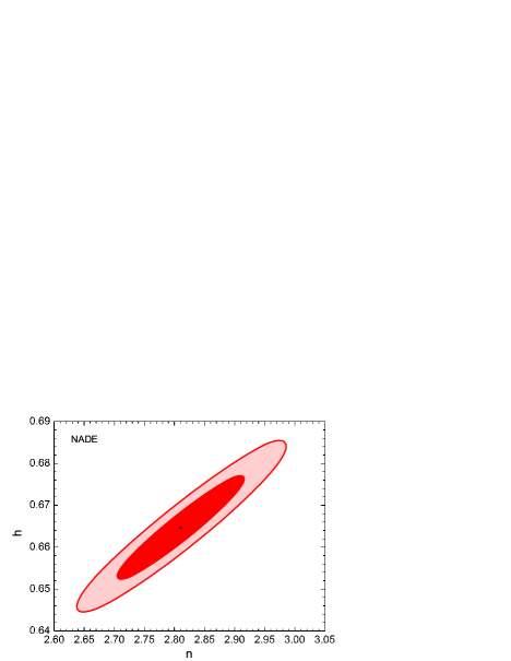
Using the MCMC method, we finally find the best-fit parameters: $n=2.810^{+0.113}_{-0.113}$, $h=0.665^{+0.013}_{-0.013}$ at the $1\sigma$ level, and $n=2.810^{+0.186}_{-0.185}$, $h=0.665^{+0.022}_{-0.021}$ at the $2\sigma$ level. The best fit gives $\chi^{2}_{\rm min}=577.451$ and $\Omega_{m0}=0.268$. In Fig. 1, we plot the contours of $1\sigma$ and $2\sigma$ confidence levels in the $n$–$h$ plane for the NADE model with the new initial condition.

The obtained results show that with the new initial condition, the observational constraints on the single parameter $n$ of NADE model are fairly tight. Next, we would like to compare the results of this work with those of previous works. We choose the work in Ref. [9] to make a comparison. Note that the work in Ref. [9] is also about the observational constraint on the NADE model but based on the old initial condition, and the observational data used in Ref.  [9] also come from the Union2 SNIa, 7-year WMAP and SDSS DR7, but the method of using CMB and BAO observations is different from our present work (method (i) in Ref. [9] while method (ii) in our present work). So, the fitting results in these two works are comparable. The best-fitted $n$ and the corresponding $\Omega_{m0}$ in that work are $2.886$ and $0.265$, respectively. We see that though the values of $n$ in the two works are relatively shifted by a small number, the values of $\Omega_{m0}$ produced by the model are rather similar. For the $95\%$ limits on $n$, the work of Ref. [9] gives $2.723<n<3.055$, and the present work gives $2.625<n<2.996$. To see the influence of the values of $n$ on the model in the two works, we will make a comparison with the quantity $f(z)\equiv\Omega_{\rm de}(z)/\Omega_{m}(z)$. Using the best-fit results obtained in the two works, we find that $f(0)_{\rm new}/f(0)_{\rm old}=0.986$ and $f(2000)_{\rm new}/f(2000)_{\rm old}=4.362$. So, it is clearly seen that though the difference in the early epoch is fairly evident, the results produced in the present time are similar.

IV Conclusions

The NADE model is considered to be a single-parameter model, due to its special analytical feature $\Omega_{\rm de}=n^{2}(1+z)^{-2}/4$ in the matter-dominated epoch. Thus, once the value of the single free parameter $n$ is given, the differential equation of $\Omega_{\rm de}(z)$ can be numerically solved by using the initial condition $\Omega_{\rm de}(z_{\rm ini})=n^{2}(1+z_{\rm ini})^{-2}/4$ at $z_{\rm ini}=2000$. However, this initial condition is only applicable in a flat universe with only dark energy and pressureless matter. That is to say, when we need to consider the contribution from the radiation, this initial condition becomes invalid. On the other hand, some cases indeed need us to consider the contribution of radiation, for instance, when using the CMB and BAO data to constrain dark energy models. We mainly have two methods: (i) using the shift parameter $R$ from the CMB and distance parameter $A$ from the BAO, (ii) employing the distance prior including $R$, $l_{A}$ and $z_{*}$ from the CMB and $r_{s}(z_{d})/D_{V}(z)$ from the BAO. Of course, method (ii) encodes more information of the CMB and the BAO observations. However, method (ii) requires us to consider the contribution from the radiation.

Thus, in order to utilize method (ii) to fit CMB and BAO data, we thoroughly analyzed the NADE model in a flat universe with dark energy, matter, and radiation. Finally, we found a similar analytical solution, $\Omega_{\rm de}=\frac{n^{2}(1+z)^{-2}}{4}\left(1+\sqrt{F(z)}\right)^{2}$ with $F(z)\equiv\frac{\Omega_{r0}(1+z)}{\Omega_{m0}+\Omega_{r0}(1+z)}$, in the early epoch (matter-dominated or radiation-dominated epoch). For the initial $z$, we still chose $z_{\rm ini}=2000$. Hence, we have a new initial condition $\Omega_{\rm de}(z_{\rm ini})=\frac{n^{2}(1+z_{\rm ini})^{-2}}{4}\left(1+\sqrt{F(z_{\rm ini})}\right)^{2}$ at $z_{\rm ini}=2000$. Furthermore, we found that this new initial condition is also applicable in a non-flat universe.

For solving the differential equation of $\Omega_{\rm de}$ before knowing the value of the non-independent parameter $\Omega_{m0}$, we provided two methods. The first method is to consider the non-independent parameter $\Omega_{m0}$ as a variable and use the new initial condition to solve the partial differential equation of $\Omega_{\rm de}$. The second method is a numerical iteration method. Our practice shows that its convergence speed is very fast. With the two methods, we have constrained the NADE model by using the new initial condition and the observational data including the Union2 SNIa, CMB from 7-year WMAP and BAO from SDSS DR7. Our fitting results show that the values of $n$ and $h$ can be constrained tightly: $n=2.810^{+0.113}_{-0.113}$, $h=0.665^{+0.013}_{-0.013}$ at the $1\sigma$ level, and $n=2.810^{+0.186}_{-0.185}$, $h=0.665^{+0.022}_{-0.021}$ at the $2\sigma$ level. The best fit gives $\chi^{2}_{\rm min}=577.451$ and $\Omega_{m0}=0.268$. We believe that our new initial condition will play a crucial rule in constraining the NADE model in the future work.