Localized O6-plane solutions with Romans mass
Fabio Saracco and Alessandro Tomasiello
Dipartimento di Fisica, Università di Milano-Bicocca, I-20126 Milano, Italy
and
INFN, sezione di Milano-Bicocca, I-20126 Milano, Italy
Abstract
Orientifold solutions have an unphysical region around their source; for the O6, the singularity is resolved in M-theory by the Atiyah–Hitchin metric. Massive IIA, however, does not admit an eleven-dimensional lift, and one wonders what happens to the O6 there. In this paper, we find evidence for the existence of localized (unsmeared) O6 solutions in presence of Romans mass, in the context of four-dimensional compactifications. As a first step, we show that for generic supersymmetric compactifications, the Bianchi identity for the RR field follows from constancy of . Using this, we find a procedure to deform any O6–D6 Minkowski compactification at first order in . For a single O6, some of the symmetries of the massless solution are broken, but what is left is still enough to obtain a system of ODEs with as many variables as equations. Numerical analysis indicates that Romans mass makes the unphysical region disappear.
1 Introduction
For a long time, string theory was unsatisfactory in that its definition was only perturbative in the string coupling . Fortunately, the duality revolution of the mid-’90s allowed to understand the strong coupling limit of almost all perturbative definitions of string theory. In particular, the strong-coupling limit of IIA was realized to be eleven-dimensional supergravity.
Actually, there is a fly in the ointment, which is the reason we wrote “almost”. Whenever the so-called Romans mass is present, the duality between IIA and eleven-dimensional supergravity does not work any more. Moreover, since is simply one of the field strengths in the theory, this “massive” version of IIA can be connected to the ordinary, “massless” version by domain walls: the D8-branes.
In [1], it was shown that, for classical solutions of massive IIA, the string coupling is bounded by the curvature in string units. In a sense, this makes the problem more rare: any solution with large is already invalidated by being strongly curved. This makes the need for a non-perturbative completion less pressing.
There do exist, however, solutions for whose existence we have independent arguments, which are less easy to dismiss in spite of being strongly curved. One example is the supergravity solution for the D8-brane itself. In this solution, the string coupling on the brane is a free parameter, and it can be made large. This is not in contradiction with the general argument in [1], because at the same time the solution becomes strongly curved. But in this case we do expect the solution to survive in fully-fledged string theory, because of its open-string interpretation and because it is half-BPS. Similar considerations apply to other configurations such as D4–D8 systems.
For D6-branes and O6-planes, however, the situation is less clear. O6-planes are of particular theoretical interest because of the way they get resolved by M-theory. The metric in the massless theory reads
| (1.1) |
Even if we excise the unphysical “hole” , the metric becomes singular for . Of course, probing the metric at such small distances was unwise to begin with: if is small, is smaller than the string length . If is large, we may try and use M-theory, with the customary formula for the eleven-dimensional lift (and knowing that the dilaton is given by ). The metric is Ricci-flat, but it is still singular at . Quantum effects, however, correct this metric at small to the so-called Atiyah–Hitchin metric [2, 3]. This metric still has a minimum allowed value for the radial variable, but it is now at , and the geometry there is smooth.
So the singularity of the massless O6 solution (1.1) is resolved in M-theory to a smooth hole. What about O6-planes in massive IIA? Solutions of this type have been assumed to exist, especially in the context of flux compactifications. A popular trick in supergravity is to “smear” sources over the internal manifold; namely, to replace the localized source with one which is spread all over space. For an orientifold plane in string theory, this is not really physically allowed, since such sources are supposed to sit on the fixed loci of the orientifold involutions. Nevertheless, smeared solutions are often a good indicator of whether a bona fide background will exist. Using this sleight of hand, quite a few massive O6 solutions have been found. A well-known early example [4, 5]111The localization of smeared sources was analyzed in [6], in different setups from the one we consider here. of moduli stabilization is of this type. Also, the presence of both O6’s and is considered the most promising avenue for producing de Sitter vacua in string theory which are completely classical (as opposed to de Sitter vacua such as [7, 8]); examples with the smearing trick include [9, 10].
It would be interesting, then, to check whether such massive O6-planes really do exist as localized solutions, and if so, what happens to the unphysical hole around their source.
In this paper, we will find evidence for the existence of supersymmetric massive O6-plane solutions. We will mostly consider a spacetime of the form
| (1.2) |
since we have already at least the example [4, 5], which is of this form. The O6 will be filling the four-dimensional spacetime, as well as three of the six directions in . We will also consider the possibility ; however, we do not know of any supersymmetric Minkowski compactification with O6-planes and Romans mass, and for this reason we will give more attention to (1.2).
Actually, although some of our considerations will be more general, as we get more concrete we will focus on what happens close to the O6 source, so that we can forget about the details of the internal topology; in practice, this just means taking . We cannot expect the geometry on this to approach flat space, however, as would be the case if one factorized the metric (1.1) as . This is because neither nor are vacua for the massive theory. So taking just means that we are focusing on what happens close to the O6 source; there is really no such thing as a massive O6 solution ‘in flat space’. Still, one can arrange so that the deviations from flat asymptotics happen at large distances. We are introducing two new length scales: and (since always appears multiplied by in the equations of motion). When both of these scales are large, it is possible to study the features of the geometry closer to the source (order ).
Let us now summarize our results, and give a synopsis of the paper. In section 2, we give a very condensed review of the “generalized complex geometry” approach to supersymmetry, which we will use in the rest of the paper. This formalism divides all possible supersymmetric vacua into three classes, of which only two are relevant here: SU(3) structure, and structure. The massless O6 solution, whose metric we gave in (1.1) and which we review at greater length in section 3, is of the first type; so is the smeared massive O6 solution of [4, 5], which we review in section 4. A very simple argument, however, shows that the localized (that is, unsmeared) massive O6 solution we are looking for should be of structure type.
Hence, in section 5, we apply the generalized complex formalism of section 2 to the structure case. We find handier expressions for the RR fluxes than were available so far; this allows us to show that the Bianchi identity for follows from that of (which simply requires to be constant). This turns out to be very useful later on; in particular, it is crucial for our first-order deformation in section 6. This is a simple procedure to deform any SU(3) structure Minkowski solution into an AdS solution, at first order in
| (1.3) |
(where is the cosmological constant).
Any Minkowski solution obtained as back-reaction of an O6–D6 system on a Calabi–Yau is of SU(3) structure type222In fact, conversely, all known smeared Minkowski solutions can be obtained as O6–D6 systems on Calabi–Yau’s, up to duality.. So we can apply the first-order deformation procedure to any such configuration. To go beyond first-order, however, we need to have more symmetries, and for this reason in section 7 we focus on the neighborhood of an O6 source, in the sense explained earlier.
Actually we find (in section 7.1) that already the first-order solution has a smaller symmetry group than the massless O6 solution. This smaller group is fortunately still large enough to reduce the problem to a system of ODEs. As we show in section 7.3, this turns out to have as many variables as equations (thanks in part to the result in section 5 about the Bianchi identity of ), and is thus expected to admit a solution. We performed both a perturbative and a numerical study. The latter seems to work well enough to infer some properties of the solution.
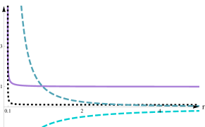
In particular, we find that the unphysical “hole” around the orientifold source gets resolved by the Romans mass; see figure 1. For , , we recover the massless O6 solution (1.1), as we should; raising both these quantities in an appropriate way, the unphysical region disappears, while the string coupling and the curvature stay small.
For the theoretical status of massive IIA, this is a very satisfying outcome. Massless O6 solutions have an unphysical region around their sources, which gets resolved by M-theory; in the massive theory, there is no lift to M-theory, but massive O6 solutions do not have the unphysical region to begin with.
The that surrounds the O6 does not shrink as : it remains of finite size. It is possible, however, to continue the metric analytically with essentially another copy of the same geometry.
2 Supersymmetry
We will begin by reviewing in this section the conditions for unbroken supersymmetry for four-dimensional compactifications, using the language of generalized complex geometry.
2.1 The equations in general
We will consider a spacetime of the warped-product form
| (2.1) |
where is the metric for either Mink4 or AdS4, is the metric on the internal manifold (which is otherwise left arbitrary) and is a function of called warping.
Such a geometry is supersymmetric in type IIA333The conditions for type IIB, that we do not need here, are obtained by . if and only if [11, Sec.7]
-
•
There exists an structure on . Here, are polyforms which are pure spinors for Clifford, and which satisfy
(2.2) for any . We have used the Chevalley–Mukai internal product between internal forms: , .
-
•
There exist a closed three-form , and an even-degree polyform (the sum of all the internal fluxes) such that [12, 13]
(2.3a) in the Minkowski case, and [14] (2.3b) in the AdS case. Here, is the cosmological constant (as we already saw in (1.3)), and . is a delta-like source supported on branes or orientifolds. is an algebraic operator that depends on alone; it is reviewed for example in [13, Sec. 2.1]. In section 2.2 we will give its explicit expression for the cases we are interested in.
Neither the metric , nor the dilaton , nor the spinorial parameters of the supersymmetry transformations, appear directly in (2.3). Moreover, we will soon see that the which does appear is not actually the physical NS three-form. Rather, there is a one-to-one correspondence between solutions of the algebraic conditions (2.2) and the geometric data we just mentioned:
| (2.4) |
In particular, we will call
| (2.5) |
the two-form determined by (2.4). For more details on this correspondence, see [15, 11]. These data are not really needed to solve (2.3). However, for completeness we will give in section 2.2 the explicit formulas for in terms of for the cases that we are interested in.
(2.3) is invariant under the transformation444This property is the main reason we are using the system (2.3) rather than the original form of these equations [12, 11], involving the Hodge star. Those equations can be made invariant under (2.6) only after defining a rather awkward operator.
| (2.6) |
As it turns out, the determined by via (2.4) transforms as under (2.6). The physical NS three-form is the combination
| (2.7) |
which is thus invariant under (2.6). The physical RR field is the one which obeys :
| (2.8) |
2.2 Solving the algebraic constraints
We will now analyze the algebraic part of the supersymmetry equations, (2.2).
There are three cases to consider. Let us call the type of a pure spinor the smallest degree that appears in the sum; in other words, only contains forms of degree type or higher. It turns out that the type of a pure spinor in dimension 6 can be at most 3. There are then three cases:
-
1.
has type 0, and has type 3. This is usually referred to as the “ structure” case, for reasons that will become clear soon.
-
2.
has type 0, and has type 1. This is the most generic case, and for this reason it is sometimes just called “”, or also “intermediate SU(2) structure”.
-
3.
has type 2, and has type 1. This is called “static SU(2) structure” case.
In this paper, we will only need the first two cases.
2.2.1
We will start by giving the solution of the algebraic constraints in (2.2) in the SU(3) structure case. The condition of purity on each separately determines (up to a -transform)
| (2.9) |
with and real functions, a non-degenerate real two-form, and a decomposable three-form (one that can be locally written as wedge of three one-forms) such that is never zero555We are including in the definition of purity.. The constraint (2.2) then reduces easily to
| (2.10) |
These equations define an SU(3) structure, which justifies the name given earlier to case 1.
We will now describe the map (2.4) for this case. The obtained by it is zero:
| (2.11) |
The metric defined by (which, once again, is not needed in the system (2.3)) can be described as follows. , being decomposable, determines an almost complex structure (it is the one such that is a -form). Then we write . The condition (2.10) implies that the defined in this way is symmetric. Finally, the dilaton is given by
| (2.12) |
We also give the form of , which enters (2.3):
| (2.13) |
2.2.2
In this case, one can parameterize the most general solution to (2.2) as [16, 17, 18]
| (2.14a) | ||||
| (2.14b) | ||||
where
| (2.15) |
for some (varying) angle , real function , one-form and two-forms satisfying
| (2.16) |
which mean that define an SU(2) structure.666Actually, from the constraint (2.2), one would get (2.16) wedged with , but one can show [18, Sec. 3.2] that these can be dropped without any loss of generality. These can also be rewritten more symmetrically as
| (2.17a) | |||
| (2.17b) | |||
these equations are reminiscent of the defining relations of the quaternions , which is ultimately because SU(2)Sp(1). Finally, the inequality in (2.2) implies that the top-form should be non-zero everywhere.
We will now detail the map (2.4) for this case. This can be inferred by comparing (2.14) to its derivation in [16, 17, 18] from spinor bilinears. For example, [18, Eq. (3.19)] can be connected to (2.14) by a -transform; from this, we see that the defined by (2.4) is non-zero:
| (2.18) |
The metric can be found by relating the forms , and in (2.14) to the spinor bilinears of an SU(3) structure. In [18] one finds , , where . This tells us that the metric is the direct sum of a two-by-two block , and of a four-by-four block determined by the SU(2) structure , . In other words, we have two orthogonal distributions (namely, subbundles of ): and . The explicit form of the four-by-four block in the metric is , where is an almost complex structure along . This means that squares to -1 along :
| (2.19) |
where is the projector on . We should now compute . This can be done by writing (which can be derived in holomorphic indices). Since only spans four directions, has rank 4; so writing is an abuse of notation. It should be understood as an inverse along the distribution . In practice, it can be computed as a matrix of minors:
| (2.20) |
Putting all together, we have
| (2.21) |
3 O6 solution
In this brief section, we will review how the O6 solution in flat space, whose metric was given in (1.1), solves the system (2.3a).
The internal space is in this case nothing but , with coordinates and (to be thought of respectively as parallel and orthogonal to the O6).
The O6 solution is of -structure type (2.9). For cosmological constant , and hence , the equations in (2.3a) read
| (3.1) | ||||
| (3.2) |
Notice that, in this case, is constant, but otherwise undetermined.
In general, in (3.1) is a delta-like current supported on the sources present. For the O6 solution, it reads
| (3.3) |
an SU(3) structure that solves (3.1) can then be given as
| (3.4) |
with the Green function for the flat Laplacian in :
| (3.5) |
as we already saw in (1.1).888If we had had D6-branes instead of an O6-plane, the function would have read , with . We also have
| (3.6) |
is a constant that we can think of as the value of at infinity.
The SU(3) structure in (3.4) is one possible solution to (3.1), and by itself it only describes four supercharges; there are other solutions, related to the one in (3.4) by flipping some signs, which describe the other supercharges. In this paper, we will focus on (3.4) and ignore the SU(3) structures: for this reason, our massive solutions will have supersymmetry.
Finally, notice that, since the solution stops making sense before we can get to , the equation has to be understood as a Gauss’ law: namely,
| (3.7) |
for any that surrounds the origin, where the O6-plane is located.
4 Smeared O6 with Romans mass
Our aim is to find a O6 solution in the presence of Romans mass. As recalled in the introduction, a solution of this type can be found easily if one “smears” the O6 source; this was done in [4] in the language of effective field theory, and lifted to ten dimensions in [5].
We take a spacetime of the form (1.2): the four-dimensional part has non-zero cosmological constant. This means that , and thus we have to use the version (2.3b) of the supersymmetry conditions. If we also take
| (4.1) |
we get999The first two equations in (2.3b), which are the ones that are equivalent to the conditions of unbroken supersymmetry, do not by themselves imply that . For the Romans mass they would give ; if one now also adds the Bianchi condition , one gets that is constant. In (4.2) we set it to zero, because a non-zero value can always be reabsorbed in the definition of .
| (4.2) |
From (2.12), it also follows that the dilaton is constant; .
So far, the source was unspecified. To find the solution in [4], take . Then we see that the Bianchi identity for implies
| (4.3) |
This is the “smearing” proposed in [5].
To get a sense of the physics of this compactification, let us moreover assume as in [4] that is of order one, that the periods of are of order , and that the internal space has volume . We know already that ; it makes sense to fix the proportionality constant as
| (4.4) |
so that integrating along a 3-cycle gives an order one number. The Bianchi identity then says ; moreover, from (4.2) we see that and . We thus find that the parameters scale as
| (4.5) |
We have seen that it is easy to find a supersymmetric solution including O6 planes and Romans mass, if one is willing to smear the O6 source as in (4.4). As stressed in the introduction, smearing an O6 is not really meaningful in string theory, but solutions obtained with this trick are often precursors to “localized” solutions, namely ones where the source is delta-like as it should be (as in (3.4)). So we can take the solution reviewed in this section as an inspiration for the solution we are looking for.
The most natural course of action might seem to solve the equations (4.2) without assuming , and with an unsmeared source, unlike in (4.4). However, we immediately face a problem: (4.2) imposes . This does not seem possible for a solution with a source: in particular, the solution with has a non-constant , as we can check from (3.6).
So unfortunately we cannot use SU(3) structure solutions. We are left with the cases 2 and 3 in section 2.2. If we think of adding a small amount of to the massless solution, which is SU(3), it seems more natural to select case 2, which is generic and can be continuously connected to the SU(3) structure case, rather than case 3, which is isolated. This is the reason we did not study case 3 in section 2.2. In section 2.2.2 we reviewed the solution (2.14) of the algebraic constraints (2.2) for case 2; we will now analyze the corresponding differential equations.
5 structure compactifications
As we just saw, a localized O6 with Romans mass cannot be an SU(3) structure solution; this motivates us to look for an structure solution. For that class, the algebraic constraints have been reviewed in section 2.2.2; we will now use those results (in particular (2.14)) in the system (2.3). This section contains both a review of old results, and some new ones — most importantly, the expressions for the fluxes.
For reasons explained in the introduction, we will first look at the AdS case, which we divide in two sections, 5.1 and 5.2. We will then also analyze the Minkowski case, in section 5.3.
5.1 AdS: generic case
5.1.1 Geometry
We will start by the first equation in (2.3b), . Using (2.14), the one-form part says that
| (5.1) | ||||
| (5.2) |
In deriving (5.2), we have solved (5.1) by taking
| (5.3) |
where is a constant. This means that we have assumed
| (5.4) |
everywhere. In this subsection, we will continue our analysis in this assumption. The case is quite different, and will be described in section 5.2.
5.1.2 Flux
We will now look at the second equation in (2.3b). We have seen that is determined by (5.5). We can then use (2.6) with the choice , so that we end up with in (2.3b).
However, there is a price to pay. Once we transform , we also have to transform the associated operator :
| (5.7) |
For the choice , remembering (2.23), we get that the new operator is
| (5.8) |
This can be computed in two ways. The first is to compute the associated action on , where is represented by . The second is to just use the formula , and
| (5.9) |
as an example of the usual Lefschetz representation of on forms (see for example [19, Ch. 0.7]). Either way, we get
| (5.10) |
We can now compute the fluxes from the second equation in (2.3b):
| (5.11a) | ||||
| (5.11b) | ||||
| (5.11c) | ||||
| (5.11d) | ||||
Recall that is related to the dilaton by (2.22). The expression for already appeared in [14]. The expressions for and are new; their expressions appear much simpler than in earlier computations, thanks in part to the transformation we performed earlier.
Notice that the Bianchi identities for (5.11) are now , away from sources. The one for just says is constant, as usual. If we now consider , we see that the term not multiplying is exact, so it drops out. On the other hand, the form that multiplies is easily seen to be closed as a consequence of (5.6). So we conclude
| (5.12) |
In other words, the Bianchi identity for is redundant. This fact will be very important for the rest of this paper.
5.2 AdS: special case
We will again start by the first equation in (2.3b), . Our generic analysis in section 5.1 relied on the assumption that ; in this section we will consider the case
| (5.15) |
This obviously solves (5.1). The remaining one-form equation now says
| (5.16) |
which replaces (5.2).
The three-form part of now gives
| (5.17) |
Finally, the five-form part can be shown to follow from the one- and three-form parts, (5.16) and (5.17).
We now turn to the RR fluxes. Unlike in section 5.1.2, this time there is no natural -transform to perform, because given in (5.17) is not necessarily exact. So we will give the expressions of the fluxes which are closed under , rather than under :
| (5.18a) | |||
| (5.18b) | |||
| (5.18c) | |||
| (5.18d) | |||
Unlike in section 5.1.2, this time the flux equations for are not obviously following from the ones for , or from any other combination of equations.
5.3 Minkowski
6 A general massive deformation
Using the results of section 5, we will now point out the existence of a first-order AdS deformation of any SU(3) Minkowski solution in IIA. As we saw in the introduction, this includes any solution obtained as back-reaction of O6–D6 systems in IIA — although in section 7 we will specialize it to the case of a single O6 in . The expansion parameter is . This deformation should not be taken as a modulus: as we will see below, the fluxes we will introduce contain , and flux quantization will in general discretize it. Rather, our expansion is to be understood as a formal device to establish the existence of a solution at finite .
We will start by determining how should be deformed. As we remarked after (3.2), this parameter is an undetermined constant for the O6 solution we want to deform. However, we would like our solution to have something to do with the DGKT solution we reviewed in section 4. More specifically, we would expect our solution to approach the DGKT solution far from the source. Remembering (4.1), we will take to be small. Since our deformation parameter is , we might then take to be of order .
This decision seems to run into trouble, however, as soon as we consider (5.2). If is of order , seems to diverge as , whereas we need it to go to zero.
To cure this potential disaster, we need at least two more factors of in the numerator of (5.2). One can try to postulate that these extra factors are somehow supplemented by the derivative. This leads us to
| (6.1) |
As in [20], we also suppose that everything is either odd or even in , so that whatever function or form is already non-zero before the deformation will be unchanged at first order. This means, in particular, that we do not change the dilaton, internal metric and warping given in section 3. This gives
| (6.2) |
Also, since now is introduced at first order, we can mimic the procedure in [20, Sec. 4.1] and use it to deform an SU(3) structure into an structure. The conclusions reached in that reference can be summarized as follows. The function and the one-form start at first order:
| (6.3) |
the pure spinors have the form
| (6.4) | |||
| (6.5) |
Comparing the order part of with (2.9), we get
| (6.6) |
which means, in particular, that is a form with respect to the almost complex structure defined by the three-form of the SU(3) structure solution. This can be used to derive the imaginary part of :
| (6.7) |
where is the action of the almost complex structure determined by , and is the corresponding Dolbeault operator. Finally, notice that (6.6) can be inverted by writing
| (6.8) |
So far we have only looked at equation (5.2) and to the algebraic constraints on the pure spinors . We now turn to the other differential equations, starting with the ones that constrain the geometry.
The first equation we consider is (5.1), that at first order simply reads . In view of (2.22), this is consistent with our postulate that and should not be deformed at first order. Comparing with (5.3), we see that is an odd function of :
| (6.9) |
We have called the first coefficient in the expansion , so as to conform with the value of in the particular solution (3.6).
Equation (5.6) is more problematic, because of the in the denominator that makes the perturbation series start at order in the left-hand side. Enforcing again our policy that all our power series in be either even or odd function of , we can expand up to second order:
| (6.10) |
Equation (5.6) is then, at order ,
| (6.11) |
This is one of the equations in the system we are deforming, as we can see from (3.1). At order , (5.6) then gives
| (6.12) |
As we will see, this equation is the only one we will encounter in which appears at all, so at this order has nothing else to satisfy. The right hand side is automatically closed, because of (3.2); but saying that it should be exact is a possible obstruction to deforming a given SU(3) structure Minkowski solution.
We will now look at the fluxes. Our formula for , (5.5), has a in the denominator, just like (5.6). That would again force us to start our perturbation theory with negative powers of . In this case, however, we can actually use (5.6) to rewrite so that it starts at first order:
| (6.13) |
Notice that the first term in is the same as the one for in the SU(3) structure solution given in (4.2), and the second term vanishes wherever tends to a constant.
As for the RR fluxes, only and will be generated at first order; will keep the same expression it had at zeroth order, (3.2). is given by
| (6.14) |
We have expanded (5.11a) at first order in , and used (2.22). As remarked after (5.12), that the Bianchi identity for follows from the one for . So the only Bianchi identity we have to impose at first order is that
| (6.15) |
For completeness, however, we also give here the expression for . Actually, the Laurent series for in (5.11c) starts with a term , which diverges like . So only becomes finite once one considers a finite . This is not terribly worrying: as we anticipated at the beginning of this section, the expansion in is simply a formal device to establish the existence of a solution at finite . In any case, the terms disappear if we go back to the , which are closed under . We get
| (6.16) |
Let us now summarize this section. We found a first-order perturbation of an SU(3) Minkowski solution which turns it into an AdS solution of type. The perturbation parameter is . The only input is the function in (6.1), which has to satisfy (6.15). One also has to solve (6.12), but this simply requires to invert .
We are now going to apply this first-order deformation to O6 solutions.
7 Massive O6 solution
In section 6, we have found a procedure to deform any SU(3)-structure Minkowski solution at first order in . In this section, we will try to promote this deformation to a fully-fledged supergravity solution.
Although the first-order deformation procedure can potentially be applied to any O6–D6 system, we will focus on the region around a single O6. This means that we will take the internal manifold to be , with a single localized source as in (3.3). By doing this, we gain more symmetries than would be available for a general O6–D6 system; that will help us solve the system.
However, as we anticipated in the introduction, this should not be understood too literally as a massive O6 “in flat space”. Unlike for (1.1), in the massive case the metric will not approach flat space far away from the source, simply because flat space is not a solution in the massive case. There are two new length scales associated with the massive problem, and , and the deviations from flat space asymptotics will become apparent at distances of the order of the smallest of these two length scales. The solution of this section should be thought of as a “close-up” around an O6 source in an geometry where is compact — so the large -behavior will not too important.
After some preliminaries in section 7.1, in section 7.2 we will specialize the general procedure of section 6 to a single O6. In section 7.3 we will then promote it to a finite deformation; this will culminate in the numerical study of section 7.3.4, where we will find numerical solutions and describe their physical features, some of which were described in the introduction. We will also study the system at higher order in perturbation theory, in section 7.4. In section 7.5 we will show that choosing in the pure spinors (2.14) does not lead to a solution. Finally, in section 7.6 we will look briefly at the system for the Minkowski case; we also found numerical solutions in this case, but they do not seem to satisfy flux quantization. Moreover, we do not know of any Minkowski compactification that uses this ingredient. We will not describe these solutions in as much detail as the AdS ones.
7.1 Symmetries
As in section 3, we will denote by the coordinates parallel to the O6, and by the coordinates transverse to it.
The massless O6 solution is symmetric under rotations of the three , rotations of the three , and translations in the :
| (7.1) |
It is already clear that the massive solution will not be symmetric under the whole group (7.1). As we have argued in section 4, we need to consider an solution. One of the data in its definition is a complex one-form ; as we saw in section 2.2.2, the algebraic constraints in (2.2) demand in particular that everywhere. So the real and imaginary part of are two linearly independent one-forms. However, the only linearly indepedent one-form which does not break any of the symmetries in (7.1) is
| (7.2) |
7.2 First order deformation
We will still demand that translation along the three internal coordinates parallel to the O6 should remain a symmetry. This will not be valid for a solution where there are several O6 sources, such as the one reviewed in section 4. However, this invariance will be restored when we get closer to an individual O6, which is the focus of the present paper.
Since everything can only depend on the transverse coordinates , from now on we will use the notation
| (7.3) |
Using (6.2) and (6.7), we then have
| (7.4) |
Since depends on only, we have , and is proportional to
| (7.5) |
which breaks the symmetries (7.1) of the massless O6 solution, as anticipated in section 7.1. Indeed, the one-form (7.5) is neither invariant under either the SO(3) that rotates the transverse , nor under the SO(3) that rotates the parallel . It is still invariant, however, under the diagonal SO(3) that rotates both the and the simultaneously. Also, it is still invariant under translations along the , as we stipulated at the beginning of this section. So (7.4) breaks (7.1) to
| (7.6) |
It is not hard to list all the possible forms invariant under (7.6); we have done so in appendix A. We will see that the rest of the solution respects this smaller symmetry group.
Let us now go back to applying the first order procedure of section 6 to the O6 solution.101010As remarked in section 3, we will deform one particular SU(3) structure which solves (3.1); for this reason, our massive solution will have only four supercharges, or in four dimensions, just like the solutions in [4, 5]. Incidentally, it is easy to show that any supersymmetric SU(3) structure solution with Romans mass has only four supercharges. The next step is to impose (6.15), namely that , calculated at first order, is constant:
| (7.7) |
where , and is the value of at infinity in the unperturbed solution (3.6). Explicitly, using (3.5), we get
| (7.8) |
setting to zero an inconsequential integration constant.
The other equation to be solved is (6.12). This can be inverted to give
| (7.9) |
where a prime denotes . We have used the two-forms defined in (A.2); those forms are invariant under (7.6), as promised. The constant and the function are as yet undetermined.
At this point, we have already demonstrated the existence of a solution at first order. For completeness, however, let us also give the physical fluxes explicitly. First of all, we can determine from imposing that . Looking at the expression of in (2.15), this can be done by checking that ; we get
| (7.10) |
Now we can compute the first-order fluxes and from (6.13), (6.16):
| (7.11) | ||||
As already stressed, the flux will not get deformed at first order in .
Let us now pause to consider the properties of the first-order solution we have just obtained. First of all, we note that we have a certain freedom: we have left undetermined a function in (7.9), which does not enter in the fluxes, and a constant , defined in (6.14) as the ratio between the deformation of and . Let us see what happens if we set
| (7.12) |
inspired by (4.2), which is valid for SU(3) structures. We see that we cancel the term in (7.8), which now goes linearly. One can then check that
| (7.13) |
in other words, far from the O6 source the solution approaches the SU(3) solution in (4.2).
The perturbative procedure, however, can only work in an appropriate regime. We have already determined in (7.9). Since actually grows with , seems to grow large at large , thus invalidating the first-order procedure. If , for example, we see from (7.8) that grows linearly; if , since , and recalling that , we have that the perturbation procedure is valid only if
| (7.14) |
We are not necessarily interested, however, in what happens outside this region, because eventually we want to compactify the six “internal” directions, and in particular the three directions . In the smeared solution we reviewed in section 4, we see from (4.5) that the compactification radius in string units goes like , whereas . In other words, the perturbative procedure breaks down for distances of order , which are much larger than the compactification radius .
In any case, we are now going to set up the study of the system of differential equations at all orders, guided by the results of this section. We will come back to perturbation theory in in section 7.4.
7.3 Full solution
We now want to check whether the solution we just found at first order in survives beyond first order. We are not going to use perturbation theory in this section; we will go back to using it in section 7.4.
7.3.1 Variables
At first order, the whole solution was determined by a single piece of data, the function in (6.1), which then has to solve (6.15).
Beyond first order, however, the input data are many more: the functions , and the forms , , , in (2.14), as well as the warping function in (2.1). At first order, the continuous symmetry (7.6) emerged, and we are going to assume that it is not broken in the full solution. This means that we should expand in terms of the one-forms (A.1), and , in terms of the two-forms (A.2).
There is also a discrete symmetry that we can use to our advantage. The solution we are looking for contains an O6, which is defined by quotienting the theory by the symmetry , where is the world-sheet parity, is the fermionic number for left-movers, and
| (7.15) |
is the inversion in the three directions. The pure spinors should then transform as [21]
| (7.16) |
where is the sign operator defined after (2.2). This implies
| (7.17) |
All the invariant forms in appendix A transform by simply picking up a sign, as detailed in table 1. Using that table, (7.17) implies
| (7.18) |
the coefficients , , , are now all real.
7.3.2 Algebraic equations
With this parameterization in hand, we can now proceed to imposing the algebraic equations (2.16). These give:
| (7.19a) | |||
| (7.19b) | |||
Specifically, (7.19a) comes from (2.17a), whereas (7.19b) comes from (2.17b). Moreover, the requirement in (2.2) that demands111111In fact, the first two equations in (7.19a) are linear precisely because we divided by a common factor , since it cannot vanish.
| (7.20) |
Given a solution to the algebraic constraints (7.19), one can also compute the internal, six-dimensional metric associated to the pure spinors. This is not really needed in finding a solution, except for one important check: that its signature should be Euclidean. Applying (2.21), we find
| (7.21) |
where the are given by
| (7.22) |
The metric (7.21) is symmetric under ISO(3), as we argued above (7.6). If we go to polar coordinates for the , by defining as in (3.5), and
| (7.23) |
we can write (7.21) as
| (7.24) |
where is the round metric of unit radius on the in the directions (which is the one that surrounds the O6). This exhibits the metric as a fibration of the spanned by the (along which the O6-plane is wrapped) over the spanned by the , or by and the . Since the connection is a globally defined one-form, this fibration is topologically trivial. Notice that the function multiplying simplifies to
| (7.25) |
using (7.22).
7.3.3 Differential equations
The differential equations we have to impose are (5.2), (5.6), , and , where and are given by (5.11a) and (5.11b), and is given by (3.3). Recall that follows from , as pointed out before (5.12).
First of all, (5.2) gives
| (7.26) |
(5.6) is clearly odd under . From table 1, we see that there are four odd three-forms; so (5.6) has four non-trivial components. One of these turns out to be algebraic:
| (7.27) |
So is completely determined algebraically, at all orders. The other three components in (5.6) are
| (7.28) |
We now turn to the Bianchi identities. We have one first-order equation that reads After some manipulation we write it as an equation linear in the derivatives of the variables:
| (7.29) |
We also have . A priori, this would seem to have four components, since is odd under . However, closer inspection reveals that only three components are non-trivial:
| (7.30) |
The component of along can be set to zero by taking proportional to ; the proportionality constant can be fixed by requiring that it reproduces the correct factor in . This can be read off (3.6). Thus the non-trivial equations are three:
| (7.31) |
These are determined by (5.11b) in terms of the data , , , , and their first derivatives. The equations for and give two equations which are again linear in the derivatives of the variables:
| (7.32a) | |||
| (7.32b) | |||
Remarkably, by using these two equations and (7.28), one can show that the last equation in (7.31) is actually automatically satisfied.
All in all, we have three differential equations from (7.28) (coming from (5.6)), one from (7.29) (coming from const), and two from (7.32) (coming from ), for a total of six. All of these are first-order, and linear in the first derivatives.
Having counted our equations, let us now count our variables. We can use (7.26) and (7.27) to eliminate and from the system; moreover, we can use the first two in (7.19a) to eliminate and . It is less clear how to use the remaining three equations in (7.19); one possibility is to derive , and . This leaves us with the variables
| (7.33) |
for a total of seven variables. We should also notice, however, that we have not yet fixed the gauge invariance coming from reparameterizations of the radial direction:
| (7.34) |
Under these reparameterizations, the coefficients of and a priori could mix. It turns out, however, that only the coefficients of and mix; if we impose the algebraic equations in (7.19), even the coefficients along those two are proportional. So, in particular we have
| (7.35) |
whereas of course , , transform as functions.
Thus, out of the seven variables in (7.33), one is redundant because of the gauge invariance (7.34). This effectively leaves us with six variables, which is as many as the differential equations (7.28), (7.29), (7.32). So we have as many equations as variables, and we expect a solution to exist. We will now study the system numerically.
7.3.4 Numerics
The system we found in section 7.3.3 is first-order, and linear in the derivatives of our variables. We found it useful to fix the gauge invariance (7.34) by demanding to be exact at order ; namely,
| (7.36) |
with given (7.8). In other words, the terms in (6.1) are absent. This gauge makes it easier to compare the massless limit of our numerical solutions with the solution in section 3.
Also, we imposed boundary conditions at an much larger than , but much smaller than the scales and , where deviations from the massless asymptotics become apparent. Using the first-order solution in section 7.2 as a clue, we identified a family of boundary conditions (depending on and ) such that, when one takes the limit and (thus forgetting for a moment about flux quantization), one recovers the massless solution121212The family is obtained with the help of the perturbative expansion we will consider in section 7.4; actually, besides and , the family also depends on an integration constant in . This constant has no influence on the massless limit.. This works quite well, especially if one takes the limit by keeping , as in the special choice (7.12) for the first-order solution. We take all this as a check that our numerical analysis is sound.
We then increased until it satisfied the flux quantization condition , . The behavior of the solutions for is qualitatively different from the massless solution: notably, it does not display the divergence at that plagues the massless solution (1.1) — see figure 1.
We checked that the eigenvalues of the metric (7.21) remain positive in our numerical solutions.
Let us now focus on the asymptotic behavior of our solutions at . In our gauge, tends to a constant at ; numerically, one can see and also tend to constants and . We can then use the differential equations (7.28), (7.29), (7.32) to find the asymptotic behavior of the coefficients , :
| (7.37) |
where the and are constants. These are also in agreement with the algebraic constraints (7.19).
From (7.37) it follows that the in (7.21) behave as
| (7.38) |
where are non-zero constants. For the crucial combination , however, which multiplies in (7.24), from (7.25) and (7.26) we see that
| (7.39) |
thus, the divergencies cancel out, and this coefficient goes to a constant.
As , the metric (7.24) then tends to
| (7.40) |
This metric factorizes in a factor , and a five-dimensional fibration over . Thus, asymptotically we have .
For most values of , the curvature of is small, and we can trust the supergravity approximation. However, the size of the remains finite, and the metric is no longer geodesically complete. Fortunately, it is possible to perform an analytic continuation by going to polar coordinates for the . One can then see that, in the system described in sections 7.3.2 and 7.3.3, all explicit dependence on drops out; the only dependence is introduced by the way we fix the gauge freedom (7.34). One can then continue to negative values. With our gauge choice (7.36), one can see that for the metric gets continued essentially to a mirror copy of itself.
One might feel unsatisfied by the fact that the that surrounds the orientifold never shrinks to a zero size; so the O6-plane locus does not really exist in these metrics, even though all fields transform as they should under the antipodal map of an O6 projection. Even in the massless case, however, the transverse does not shrink in the smooth Atiyah–Hitchin metric (see for example the discussion in [3, Sec. 3]).
For special choices of , the curvature of gets large; in that case, the supergravity approximation breaks down. It is possible that corrections make the size of the shrink, but this is of course speculation.
7.4 Back to perturbation theory in
In section 7.2 we considered our equations to order , and found an explicit solution. In section 7.3 we analyzed the conditions for unbroken supersymmetry in the setup suggested by the first-order solution, culminating in the numerical analysis in 7.3.4. In this section we will go back to perturbation theory in , to see how explicit can the solution be made.
First, a bit of notation: we are going to expand the various coefficients and functions as a power series in , keeping the same assumptions in section 6 about which expansions contain even or odd powers:
| (7.41) |
As it turns out, the equations at order and mix quite a bit. Using the algebraic equations, we found it convenient to use the variables
| (7.42) |
For example, even if we have already solved at second order in (7.9), we did so only up to an unknown function . This means that one component was actually undetermined; in terms of the expansion (7.41), this remaining equation can be written in terms of the variables (7.42). At the same time, of the equations in (5.6) only two contain the variables in (7.42); the third involves variables at higher order, and we can ignore it at this level. We then have one equation const. and three equations from , just like in our discussion at all orders in section 7.3.3.
In section 7.3.3, the system of differential equations was first-order and linear in the derivatives of the variables. The perturbative system we are considering in this subsection, once we use the solution found at first order in section 7.2, is also linear (inhomogenous) in the variables themselves. This means that we can write it as
| (7.43) |
The matrix is particularly simple in the gauge , and with the simplifying assumption :
| (7.44) |
The expression for the vector is more complicated, and we see no reason to inflict it on the reader. The first three columns of (7.44) show three obvious eigenvalues; the variables , , are determined once the other three are. So the crucial part of is the lower-right block, concerning the variables , , . The eigenvalues of this block can be found by the Cardano–Tartaglia formula, and so in principle the system at this order can be solved analytically.
7.5 The special case
In section 5 we have divided the analysis of structure solutions in three cases: AdS for (the “generic” case of section 5.1), AdS for (the “special” case of section 5.2), and the Minkowski case (in section 5.3). So far, in this section we have analyzed the system in detail in the generic AdS case . We now want to go back to the other two cases. We will begin in this subsection by the special AdS case, .
We will again work with the symmetry group (7.6), for the same reasons explained in section 7.1 and 7.2. The parameterization of the forms , , is still the same as in section 7.3.1. The algebraic equations satisfied by them can still be written as in (7.19).
Since in this case in (5.17) is not already exact (as for (6.13)), we have to impose by hand that . Since is odd, the only non-zero component of this equation is the one along :
| (7.45) |
cannot be zero because of the requirement in (2.2). Also, by assumption; so we get .
We then look at , again from (5.17). This has four non-zero components, but in particular the one along tells us that
| (7.46) |
We can now go back to the algebraic system (7.19), and use that . The last equation of (7.19a) tells us that . But, both if and if , (7.19b) now tells us . This means that , which is not possible, again because of the requirement in (2.2).
Thus, in this section we have quickly disposed of the case . This case cannot lead to massive O6 solutions with the symmetry (7.6).
7.6 Minkowski
Finally, in this section we will look at the Minkowski case.
Once again, we can use the parameterization of the forms , , in section 7.3.1, whose coefficients have to satisfy the algebraic equations in (7.19).
The relevant differential equations were given in 5.3. We start with (5.19). This says
| (7.47) |
We then turn to (5.20). The first is trivially satisfied, using the symmetries of our setup. The second gives
| (7.48) |
We now turn to the Bianchi identities. They can be discussed along the lines of the AdS case in section 7.3.3. One consists in imposing that is constant, and can be written as
| (7.49) |
As in (7.31), would seem to give three equations. The ones for and read:
| (7.50a) | |||
| (7.50b) | |||
Once again, the third equation in (7.31) can be shown to be automatically implied by (7.50) and by (7.47), (7.48).
So we have one differential equation from (7.47), one from (7.48), one from (7.49), and two from (7.50). This gives a total of five differential equations, which are all first order, and linear in the derivatives.
Let us now count our variables. Unlike in the AdS case, and are now independent variables. On the other hand, (7.47) allows us to eliminate (which vanishes) and (which is a function of other variables). All in all, we can take as independent variables
| (7.51) |
Just as in section 7.3.3, we still have the gauge freedom (7.34). This means that one of these six variables is actually redundant, and we effectively have five variables.
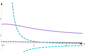
So we again have as many variables as equations. We have studied the system numerically. The solutions share some qualitative features with the ones for the AdS case (see figure 1(b)); for example, the warping stays flat rather than diverging. However, they only survive for small values of , which do not satisfy the flux quantization condition . For values of that do satisfy flux quantization, the system seems to crash in a singularity before it gets to .
It is also possible to set up a perturbative study. Since in this case, we cannot perturb in . We introduce a new perturbation parameter , such that as . This can be achieved by taking the coefficients and to be odd functions of , while the other coefficients , will be even functions of . We solved the resulting system at first order in , similarly to section 7.2.
Finally, it would presumably also be possible to deform the Minkowski solutions discussed in this section into an AdS solution, by generalizing the procedure in section 6.
Acknowledgments.
Our research is supported in part by MIUR–PRIN contract 2009-KHZKRX. We would like to thank G. Moore for his initial involvement in the project, and A. Zaffaroni for useful discussions.
Appendix A Forms
In this appendix, we will give a basis of forms symmetric under the symmetry ISO(3) we identified in section 7.2. This consists of translations in the directions parallel to the O6-plane, and of simultaneous rotations of both the and of the , transverse to the O6-plane. In the main text, we have used this basis to expand both our pure spinors and fluxes.
The one-forms are:
| (A.1a) | ||||
| (A.1b) | ||||
A 2-form basis compatible with the symmetry is:
| (A.2a) | ||||
| (A.2b) | ||||
| (A.2c) | ||||
| (A.2d) | ||||
| (A.2e) | ||||
we recalled here that the last form is nothing but the two-form of the massless O6 solution, (3.4).
The 3-forms can be written in terms of:
| (A.3a) | ||||
| (A.3b) | ||||
| (A.3c) | ||||
| (A.3d) | ||||
| (A.3e) | ||||
| (A.3f) | ||||
| (A.3g) | ||||
| (A.3h) | ||||
4-forms and 5-forms can then be obtained as wedge products from the previous definitions:
| (A.4a) | ||||
| (A.4b) | ||||
| (A.4c) | ||||
| (A.4d) | ||||
| (A.4e) | ||||
| (A.5a) | ||||
| (A.5b) | ||||
Crucially, this basis is closed under exterior derivative wedge product. One can then express both in terms of appropriate tensors: for example, the wedge product between the 2-form and the 3-form can be written in terms of a tensor :
| (A.6) |
where . The same idea can be applied to the exterior derivative. For example:
| (A.7) |
with an appropriate tensor. Working out all these tensors speeds up computations significantly.
Under the a parity transformation
| (A.8) |
in the directions perpendicular to the O6-plane, the forms defined above transform by picking up signs. This signs are summarized in table 1.
| Even | Odd | |
|---|---|---|
| 1-forms | ||
| 2-forms | ||
| 3-forms | ||
| 4-forms | ||
| 5-forms |
References
- [1] O. Aharony, D. Jafferis, A. Tomasiello, and A. Zaffaroni, “Massive type IIA string theory cannot be strongly coupled,” JHEP 1011 (2010) 047, 1007.2451.
- [2] M. Atiyah and N. J. Hitchin, “Low-Energy Scattering of Nonabelian Monopoles,” Phys.Lett. A107 (1985) 21–25.
- [3] G. Gibbons and N. Manton, “Classical and Quantum Dynamics of BPS Monopoles,” Nucl.Phys. B274 (1986) 183.
- [4] O. DeWolfe, A. Giryavets, S. Kachru, and W. Taylor, “Type IIA moduli stabilization,” JHEP 07 (2005) 066, hep-th/0505160.
- [5] B. S. Acharya, F. Benini, and R. Valandro, “Fixing moduli in exact type IIA flux vacua,” JHEP 02 (2007) 018, hep-th/0607223.
- [6] J. Blaback et al., “Smeared versus localised sources in flux compactifications,” JHEP 12 (2010) 043, 1009.1877.
- [7] S. Kachru, R. Kallosh, A. Linde, and S. P. Trivedi, “De Sitter vacua in string theory,” Phys. Rev. D68 (2003) 046005, hep-th/0301240.
- [8] V. Balasubramanian, P. Berglund, J. P. Conlon, and F. Quevedo, “Systematics of Moduli Stabilisation in Calabi–Yau Flux Compactifications,” JHEP 03 (2005) 007, hep-th/0502058.
- [9] E. Silverstein, “Simple de Sitter Solutions,” Phys. Rev. D77 (2008) 106006, 0712.1196.
- [10] U. H. Danielsson, S. Haque, P. Koerber, G. Shiu, T. Van Riet, and T. Wrase, “De Sitter hunting in a classical landscape,” Fortschr. Phys. 59 (2011) 897–933, 1103.4858.
- [11] M. Graña, R. Minasian, M. Petrini, and A. Tomasiello, “A scan for new vacua on twisted tori,” JHEP 05 (2007) 031, hep-th/0609124.
- [12] M. Graña, R. Minasian, M. Petrini, and A. Tomasiello, “Generalized structures of vacua,” JHEP 11 (2005) 020, hep-th/0505212.
- [13] A. Tomasiello, “Reformulating Supersymmetry with a Generalized Dolbeault Operator,” JHEP 02 (2008) 010, arXiv:0704.2613 [hep-th].
- [14] D. Gaiotto and A. Tomasiello, “Perturbing gauge/gravity duals by a Romans mass,” J. Phys. A42 (2009) 465205, 0904.3959.
- [15] M. Gualtieri, “Generalized complex geometry,” math/0401221. Ph.D. Thesis (Advisor: Nigel Hitchin).
- [16] C. Jeschek and F. Witt, “Generalised structures and type IIB superstrings,” JHEP 03 (2005) 053, hep-th/0412280.
- [17] R. Minasian, M. Petrini, and A. Zaffaroni, “Gravity duals to deformed SYM theories and generalized complex geometry,” JHEP 12 (2006) 055, hep-th/0606257.
- [18] N. Halmagyi and A. Tomasiello, “Generalized Kaehler Potentials from Supergravity,” Commun.Math.Phys. 291 (2009) 1–30, 0708.1032.
- [19] P. Griffiths and J. Harris, Principles of algebraic geometry. Wiley-Interscience [John Wiley & Sons], New York, 1978. Pure and Applied Mathematics.
- [20] D. Gaiotto and A. Tomasiello, “Perturbing gauge/gravity duals by a Romans mass,” 0904.3959.
- [21] I. Benmachiche and T. W. Grimm, “Generalized orientifold compactifications and the Hitchin functionals,” Nucl. Phys. B748 (2006) 200–252, hep-th/0602241.