Flashing subdiffusive ratchets in viscoelastic media

Abstract

We study subdiffusive ratchet transport in periodically and randomly flashing potentials. Central Brownian particle is elastically coupled to surrounding auxiliary Brownian quasi-particles which account for the influence of viscoelastic environment. Similar to standard dynamical modeling of Brownian motion, the external force influences only the motion of central particle not affecting directly the environmental degrees of freedom (see video). Just a handful of auxiliary Brownian particles suffice to model subdiffusion over many temporal decades. Time-modulation of the potential violates the symmetry of thermal detailed balance and induces anomalous subdiffusive current which exhibits a remarkable quality at low temperatures, as well as a number of other surprising features such as saturation at low temperatures, and multiple inversions of the transport direction upon a change of the driving frequency in nonadiabatic regime. Our study generalizes classical Brownian motors towards operating in sticky viscoelastic environments like cytosol of biological cells or dense polymer solutions.

1 Introduction

Physics of noise-assisted driven transport presents currently a well-established area of research [1, 2]. Most papers are devoted to classical transport in neglecting non-Markovian and even inertial effects. The corresponding stochastic nonlinear dynamics can be described by a Langevin equation in time-dependent potentials and/or by associated Fokker-Planck equation for the noise-averaged dynamics of the probability density of an ensemble of moving particles. Key ingredients are nonlinear dynamics in periodic potentials unbiased on average, friction and thermal noise related by the fluctuation-dissipation theorem (FDT), and an external driving which violates the symmetry of thermal detailed balance ensured by the FDT at thermal equilibrium. The emerged dissipative out-of-equilibrium directed transport is necessarily accompanied by an entropy production and related heat dissipation.

Such profoundly out-of-equilibrium transport should be distinguished from other possibilities such as transport in a running potential, where the particle remains bound to a potential well which moves in space. Basically, in this later case one does not need even a periodic potential. Any trapping confining potential $U(x)$ with a deep minimum at $x=x_{0}$ will convey a transport if this minimum is moving with velocity $v$, i.e. $U(x)$ is replaced by $U(x-vt)$. Such a “peristaltic” transport is clearly not related in essence to any entropy production and for a periodic running potential it can be symbolized by the Archimedean screw pump. This is a purely mechanical system, where both the friction and the noise are not principal for the transport occurrence. Quantum-mechanical counterparts of the Archimedean pump are also well-known [3]. A peristaltic pump can be also realized with highly overdamped isothermic thermodynamic systems operating close to thermal equilibrium, where dissipation keeps the particle fluctuating near to the potential minimum, and the energy lost due to friction is perpetually restored due to stochastic impact of the environment – the physical content of FDT. Friction plays here in fact a constructive role. Moreover, neglect of the energy gain from hot environment, at odds with FDT, is one of the common mistakes in the literature, leading to erroneous belief that one must always minimize dissipation and cool the environment in order to achieve at the highest efficiencies of isothermal engines possible. This is not necessarily so. For example, the so-called dissipationless Hamiltonian ratchets [4] cannot do any useful work at all against a load, i.e. are pseudo-ratchets with zero efficiency. A dissipative system can remain locally close to thermal equilibrium, but the form of the potential is cyclically and adiabatically slow changed by a driving force so that excess, uncompensated heat exchange between the particle and the thermal reservoir can be minimized. In this quasi-equilibrium scenario, the work required to change the form of potential (to move the minimum) can be transformed with minimal heat losses into the work against the load which opposes this potential modulation. This is why such an isothermal machine considered as a free energy transducer can in principle operate with the efficiency, defined as the ratio of the work against a load to the free energy spent to drive a working cycle, close to one [5, 6, 7, 8]. For example, the efficiencies of highly optimized biological ionic pumps as high as $0.75$ are common [9] and the efficiency of ATP synthase can approach the theoretical maximum of one [10, 11, 12].

The primary focus of this paper is different, on the thermal noise assisted transport, where the thermal noise is assumed to play a profound and constructive role. A paradigmatic example is provided here by transport in flashing potentials [13], such as one in figure 1.

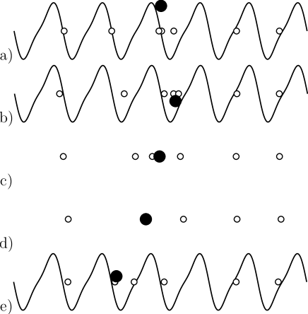
Figure 1: Snapshots of numerical simulations of the dynamics in Eq. (2.1) at different instants of time a) $t=0.1$, b) $t=0.4$, c) $t=1.6$, d) $t=2.0$, e) $t=2.5$. One Brownian particle (big filled circle) is coupled to auxiliary particles (small empty circles) at temperature $T=0.1$ and moves in a periodically flashing with frequency $\nu=1.0$ potential (15) with amplitude $U_{0}=0.75$.

In a standard Markovian overdamped setup, when the potential is off, an initially localized particle diffuses with the position variance growing linearly, $\langle\delta x^{2}(t)\rangle\propto t$, which corresponds to normal diffusion. When the potential is on, the particle relaxes to a minimum of the potential and the probability distribution becomes at least bimodal with a larger peak corresponding to sliding down a less steep side of the potential (as a larger basin of attraction corresponds to a larger distance between the minimum and maximum of a spatially asymmetric but periodic potential). When flashing repeats, either periodically or stochastically, but sufficiently slow, the net transport is expected to emerge in the left, natural direction, with the averaged particle’s position growing linearly in time. Such normal transport is characterized by mean velocity. This natural direction is opposite to one in the fluctuating tilt potential ratchets of the same potential form [14, 15]. For a fixed unbiased on average potential, the total heat exchange between the particle and its environment is zero, FDT holds, and directed transport is forbidden by the symmetry of thermal detailed balance. Out-of-equilibrium potential fluctuations violate this symmetry and induce directed transport. There emerges an overall uncompensated excess heat flow to the environment associated with the corresponding entropy production. A part of the energy put in the repeating potential flashing is dissipated as excess heat and a part can be used to do useful work against a load. If the load is absent all the consumed energy is dissipated as excess heat (futile motor) because the mechanical energy of the motor particle remains on average not changed. This is a well-established by now physical picture [16]. This basic model explains e.g. operating of single-headed kinesin motors [9], where the energy to drive stochastic cycles is provided in effect by the energy of ATP hydrolysis.

Generalization of this approach to account for a non-Markovian friction with memory is not trivial. The memory effects appear e.g. due to viscoelasticity of the environment [17, 18, 19, 20, 21, 22, 23]. Even if a corresponding Generalized Langevin Equation (GLE) [24, 25, 26, 27] is well known for any linear model of friction with the memory, the corresponding non-Markovian Fokker-Planck equation (NMFPE) [28, 29, 30, 31, 32] remains simply unknown for general nonlinear force-fields. The cases of constant force, or a linear in coordinate force, where the corresponding NMPPEs are known [28], are not especially useful in the present context. Especially interesting is the case of a power law decaying memory kernel [18] which corresponds to subdiffusion and is associated with the Cole-Cole dielectric response of viscoelastic media [33, 34]. Such viscoelastic subdiffusion has recently been found relevant also for transport in polymer networks [35, 36], cytosol of biological cells [37] and akin crowded fluids [38]. The corresponding fluctuating tilt or rocking ratchets in viscoelastic media have recently been proposed and studied in Refs. [39, 40] with a number of quite unexpected and surprising properties revealed. The interest to ratchet effect in glass-like environments is growing [41]. Flashing ratchet transport in dynamically disordered potentials was proposed and studied earlier in Ref.[42]. Transport in disordered potentials is known to be equivalent within the mean field effective medium approximation to a continuos time random walk (CTRW) approach with independent residence times in traps [43, 44, 45]. This places our research into a general context of anomalous transport processes in complex media [43, 44, 45, 46]. However, our approach to anomalous transport in viscoelastic media is very different from one based on uncorrelated CTRW. This work is devoted to flashing viscoelastic ratchets which turn out to be no less surprising than rocking viscoelastic ratchets [39, 40] and we shall take the advantage of the approach to anomalous subdiffusive transport developed recently in Refs. [22, 39, 23].

2 Dynamical approach to viscoelastic transport and stochastic modeling

We start with a well-established dynamical approach to the theory of Brownian motion [25, 27]. The environment is modeled by a set of $N_{0}$ particles with masses $m_{i}$ harmonically coupled with the spring constants $\kappa_{i}$ to the Brownian particle of mass $m$:

$$m\ddot{x} = f(x,t)-\sum_{i=1}^{N_{0}}\kappa_{i}(x-q_{i}),$$ (1)

$$m_{i}\ddot{q}_{i} = \kappa_{i}(x-q_{i})\;,$$ (2)

where $q_{i}$ are the coordinates of the environmental particles, $x$ is the coordinate of the Brownian particle, and $f(x,t)$ is an external force which affects only the motion of Brownian particle but not the environment. As usually, using the Green function of harmonic oscillator one can express the bath oscillators coordinates $q_{i}(t)$ in Eq. (2) via the initial values $q_{i}(0)$ and $p_{i}(0)$ for arbitrary $x(t)$:

$$q_{i}(t) = q_{i}(0)\cos(\omega_{i}t)+\frac{p_{i}(0)}{m_{i}\omega_{i}}\sin(\omega_{i}t)+\frac{\kappa_{i}}{m_{i}\omega_{i}}\int_{0}^{t}\sin[\omega_{i}(t-t^{\prime})]x(t^{\prime})dt^{\prime}$$ (3)

$$= [q_{i}(0)-x(0)]\cos(\omega_{i}t)+\frac{p_{i}(0)}{m_{i}\omega_{i}}\sin(\omega_{i}t)+x(t)$$

$$-\int_{0}^{t}\cos[\omega_{i}(t-t^{\prime})]\dot{x}(t^{\prime})dt\;.$$

Here, $\omega_{i}=\sqrt{\kappa_{i}/m_{i}}$ are the bath oscillators frequencies and the integration by parts has been used to obtain the second equality. By substituting (3) into (1) one immediately obtains

$$m\ddot{x}+\int_{0}^{t}\eta(t-t^{\prime})\dot{x}(t^{\prime})dt^{\prime}=f(x,t)+\xi(t),$$ (4)

where

$$\eta(t)=\sum_{i}\kappa_{i}\cos(\omega_{i}t),$$ (5)

and

$$\xi(t)=\sum_{i}\kappa_{i}\left([q_{i}(0)-x(0)]\cos(\omega_{i}t)+\frac{p_{i}(0)}{m_{i}\omega_{i}}\sin(\omega_{i}t)\right)\;.$$ (6)

Eq. (4) is still a purely dynamical equation of motion which is exact, the dynamics of irrelevant degrees of freedom is but excluded. For example, it describes a time-reversible dynamics, if external field $f(x,t)$ does not violate the time-reversal symmetry. Then the trajectories governed by Eq. (4) are also most obviously time-reversal symmetric (see [47] on this point from stochastic perspective). This is contrary to a widespread misperception. The statistical irreversibility comes about on the level of a bunch of trajectories averaged over different initial realizations of $q_{i}(0)$, $p_{i}(0)$. The loss of information due to averaging or coarse-graining is a well known source of irreversibility leading to statistical description of dynamical systems (see e.g. [49]). As a matter of fact, the dynamics described by Eq. (4) is just a projection of a highly dimensional Hamiltonian dynamics onto two dimensional $(x,p)$ phase subspace.

Furthermore, one proceeds as in a typical molecular dynamics setup. The initial positions $q_{i}(0)$ and momenta $p_{i}(0)$ of the environmental oscillators in Eq. (6) are sampled (this is the only non-dynamical element in the theory) from a canonical distribution at temperature $T$,

$$\rho(\{q_{i}(0),p_{i}(0)\}|x(0))=\frac{1}{Z}\exp\left[-\frac{1}{2k_{B}T}\sum_{i=1}^{N_{0}}\left(\frac{p_{i}^{2}(0)}{m_{i}}+\kappa_{i}[q_{i}(0)-x(0)]^{2}\right)\right],$$ (7)

conditioned on the initial position of the Brownian particle $x(0)$, where $Z$ is the statistical sum of bath oscillators. Here one assumes that initial velocities of the bath oscillators are centered at zero, i.e. the medium is not moving as whole. Likewise, the average $\langle q_{i}(0)\rangle=x(0)$, i.e. the medium is initially equilibrated adjusting to the Brownian particle localized at $x(0)$. The corresponding random force $\xi(t)$ becomes a stochastic process which is obviously Gaussian and can be completely characterized by its first two statistical moments. First moment is obviously zero, $\langle\xi(t)\rangle=0$. Furthermore, with Gaussian averages $\langle p_{i}(0)p_{j}(0)\rangle=\delta_{ij}m_{i}k_{B}T$, $\langle x_{i}(0)x_{j}(0)\rangle=\delta_{ij}k_{B}T/\kappa_{i}$, $\langle x_{i}(0)p_{j}(0)\rangle=0$ it is easy to show that

$$\langle\xi(t^{\prime})\xi(t)\rangle=k_{B}T\eta(|t-t^{\prime}|)$$ (8)

for any set of bath oscillators. This is the celebrated fluctuation-dissipation relation, or the second fluctuation dissipation theorem by Kubo [24]. The bath oscillators are conveniently characterized by the spectral density [27]

$$J(\omega)=\frac{\pi}{2}\sum_{i}\frac{\kappa_{i}^{2}}{m_{i}\omega_{i}}\delta(\omega-\omega_{i})=\frac{\pi}{2}\sum_{i}m_{i}\omega_{i}^{3}\delta(\omega-\omega_{i})\;.$$ (9)

It allows to express $\eta(t)$ as $\eta(t)=(2/\pi)\int_{0}^{\infty}d\omega J(\omega)\cos(\omega t)/\omega$ and the noise spectral density as $S(\omega)=2k_{B}TJ(\omega)/\omega$ via the Wiener-Khinchin theorem, $S(\omega)=\int_{-\infty}^{\infty}\langle\xi(t)\xi(0)\rangle e^{i\omega t}dt$. The choice $J(\omega)=\eta_{\alpha}|\sin(\pi\alpha/2)|\omega^{\alpha}$ with $0<\alpha<2$, yields the fractional Gaussian noise (fGn) $\xi(t)$ introduced by Mandelbrot and van Ness [50]. For $0<\alpha<1$ (sub-Ohmic thermal bath [27]),

$$\eta(t)=\eta_{\alpha}t^{-\alpha}/\Gamma(1-\alpha),$$ (10)

where $\Gamma(z)$ is a standard gamma function. This choice yields subdiffusion asymptotically, $\langle\delta x^{2}(t)\rangle\sim t^{\alpha}$, for an ensemble of particles [27]. The corresponding GLE (4) is termed also the fractional GLE, or FLE [51, 52, 32, 23] upon the use of the notion of fractional Caputo derivative to shorthand the frictional term, and the coefficient $\eta_{\alpha}$ is termed then the fractional friction coefficient. Such a dynamical modeling requires a very large $N_{0}\to\infty$ number of the bath oscillators with a quasi-dense spectrum.

2.1 Stochastic modeling

Alternatively, one can use just a handful of $N$ auxiliary Brownian particles clouding around the central particle [53, 23] while modeling the rest as friction and noise acting on these representative ones. Such Brownian quasi-particles can serve to model sticky viscoelastic media. A particle clouded by other particles reminds conceptually polaron picture in condensed matter physics. Then, one replaces Eqs. (1,2) with

$$m\ddot{x} = f(x,t)-\sum_{i=1}^{N}k_{i}(x-x_{i})\;$$ (11)

$$m_{i}\ddot{x}_{i} = k_{i}(x-x_{i})-\eta_{i}\dot{x}_{i}+\sqrt{2\eta_{i}k_{B}T}\zeta_{i}(t)\;,$$ (12)

where $x_{i}$ are the coordinates of auxiliary particles, $k_{i}$ are the corresponding coupling constants, $\sqrt{2\eta_{i}k_{B}T}\zeta_{i}(t)$ are thermal Gaussian forces, with zero range of correlation, $\langle\zeta_{i}(t)\zeta_{j}(t^{\prime})\rangle=\delta_{ij}\delta(t-t^{\prime})$, and $\eta_{i}$ are the corresponding friction coefficients. Moreover, the overdamped limit for these auxiliary stochastic medium oscillators, $m_{i}\to 0$, yields

$$\dot{x} = v\;,$$

$$m\dot{v} = f(x,t)+\sum_{i=1}^{N}u_{i}(t)\;$$ (13)

$$\dot{u}_{i} = -k_{i}v-\nu_{i}u_{i}+\sqrt{2\nu_{i}k_{i}k_{B}T}\zeta_{i}(t)\;,$$

where $\nu_{i}=k_{i}/\eta_{i}$ are the relaxation rates of the introduced viscoelastic forces $u_{i}=-k_{i}(x_{i}-x)$. The last equation for $u_{i}$ is similar to the Maxwell’s relaxation equation for viscoelastic force in macroscopic theory of viscoelasticity [17] which is augmented by the corresponding Langevin force in accordance with FDR. Such a description was introduced in Refs. [22, 39, 53, 23] to model anomalous Brownian motion in complex viscoelastic media within a generalized Maxwell model. For a particular case of the only one auxiliary particle (Maxwell model of viscoelasticity), the earlier description in Refs. [54, 55] leading to GLE with thermal Ornstein-Uhlenbeck noise is readily reproduced. Excluding the dynamics of auxiliary variables $u_{i}(t)$ and assuming that initially forces $u_{i}(0)$ are thermally Gaussian-distributed with zero mean and dispersion $\langle u_{i}^{2}(0)\rangle=k_{i}k_{B}T$ yields again the GLE (4) with the corresponding memory kernel presented by a sum of exponentials,

$$\eta(t)=\sum\limits_{i=1}^{N}k_{i}e^{-\nu_{i}t}.$$ (14)

The corresponding noise $\xi(t)$ presents the sum of Ornstein-Uhlenbeck noises.

The power-law memory kernel (10) can be reliably approximated by such a sum [22] over a large time-interval $[t_{l},t_{h}]$ by choosing $\nu_{i}=\nu_{0}/b^{i}$ and $k_{i}=C_{\alpha}(b)\eta_{\alpha}\nu_{i}^{\alpha}/\Gamma(1-\alpha)$. Here, $b>1$ is a dilation (scaling) parameter and $C_{\alpha}(b)$ is a fitting dimensionless constant. Physical meaning of $\nu_{0}$ is a high-frequency (short-time) cutoff of the stochastic process $\xi(t)$, $t_{l}=\nu_{0}^{-1}$. The low-frequency (long-time) cutoff corresponds to $t_{h}=b^{N-1}t_{l}$. Similar scaling and approximation to a power law are well known in the theory of anomalous relaxation [43, 56]. By adjusting $b$ and $N$ one can approximate power law over about $r=N\log_{10}b-2$ time decades. Weak dependence of $r$ on $b$ and $N$ ensures a very powerful and accurate numerical approach to FLE dynamics. Just a handful of auxiliary particles can suffice for all practical purposes. Of course, such a Markovian embedding of FLE is not unique [57]. However, it appeals by a clear physical interpretation. Recently, the set (2.1) was formally generalized to numerically integrate also superdiffusive FLE [58].

3 Flashing ratchet

To study flashing ratchet transport we take $f(x,t)=f_{0}(x)r(t)$. Here, $f_{0}(x)=-U^{\prime}(x)$ is a deterministic force acting on the particle (Brownian motor) when a potential $U(x)$ is switched on. Furthermore, $r(t)$ switches on/off taking just two values, zero and one, $r(t)=\{1,0\}$. For $U(x)$ we take a typical ratchet potential

$$U(x)=-U_{0}\left[\sin\left(\frac{2\pi x}{L}\right)+\frac{1}{4}\sin\left(\frac{4\pi x}{L}\right)\right],$$ (15)

with amplitude $U_{0}$ and period $L$. For $r(t)$ two models are considered: periodic vs. random switching. In the periodic case, $r(t)=1/2\left[1+{\rm sign}\left(\sin(2\pi\nu t)\right)\right]$, where ${\rm sign}(\cdot)$ is standard signum function and $\nu$ is linear frequency of oscillations. The first switching occurs at $t_{\rm I}=1/2\nu$ and the total number of switching is $N_{sw}\equiv T_{tot}/t_{\rm I}=2\nu T_{tot}$, where $T_{tot}$ is a total computation time which equals $N_{s}dt$; $N_{s}$ is a total number of integration steps of Eq.(4), $dt$ is a time-step. Finally, one can write $N_{sw}=2\nu N_{s}dt$. For random switching $r(t)$, we consider the model of dichotomous Markovian process (DMP) with the probability $p=2\nu dt$ to switch within $dt$. Such DMP is symmetric with equal residence time distributions in two states, $\psi(\tau)=2\nu\exp(-2\nu\tau)$. Here, $2\nu$ is transition rate from one state to another one (and also inverse of the mean residence time in a state). The mean flashing frequency $\langle\nu\rangle$ equals $\nu$.

In all simulations we scale coordinate in units of $L$ and time in units of $\tau_{v}=(m/\eta_{\alpha})^{1/(2-\alpha)}$. It is assumed to be temperature-independent in accordance with the underlying Hamiltonian model [25, 27]. This is a standard assumption done also in other ratchet models [1, 2]. Furthermore, energy is scaled in $E=L^{2}\eta_{\alpha}^{2/(2-\alpha)}/m^{\alpha/(2-\alpha)}$ and temperature $T=E/k_{B}$. In this work we choose $\alpha=0.5$ and $b=10$, $C_{1/2}(10)=1.3$, and use $\nu_{0}=100$, $N=12$. Such a set of parameters gives an excellent approximation to the FLE dynamics over at least ten time decades, until $t_{\rm max}=10^{8}$. Similar to [22, 39] this was checked by comparison with the exact analytical solution for the position variance obtained within GLE and FLE [24, 51] in the force-free case. The numerical errors due to the memory kernel approximation are negligible as compare with the overall statistical error in our stochastic simulations (several percents), see for details in [22]. Like in [40], numerical solutions of stochastic differential equations were performed on the graphical processor units (GPUs) with double precision using stochastic Heun method. The use of GPU computing allowed to parallelize and accelerate simulations by a factor of about 100, as compare with conventional CPU computing.

Schematically, viscoelastic dynamics in the flashing ratchet potential is shown in figure 1 (see also video abstract). The auxiliary particles are placed on the level $U=0$ and they are not influenced by potential. Initially, when the potential is switched on, the Brownian particle moves in the potential well (see snapshots a and b). When the potential is off (snapshots c and d) the Brownian particle “freely” subdiffuses, interacting only with auxiliary particles. After the potential is switched on again, Brownian particle moves into the next potential well (see snapshot e) with the net motion occurring in the negative direction. During such motion not all auxiliary particles follow immediately to the Brownian particle. Some of them are at large distances from the Brownian particle and are essentially less mobile than the Brownian particle and its nearest environment because they have essentially larger friction coefficient than other auxiliary particles. The weaker is the coupling constant $k_{i}$ of an auxiliary particle to the Brownian one the larger is the corresponding frictional coefficient $\eta_{i}$. These very sluggish particles create a slowly fluctuating quasi-elastic force (a temporal biasing force [22, 23]) acting on the central particle.

4 Results and discussion

In all simulations we monitored two main statistical quantities, the mean position $\langle x(t)\rangle$ and the position variance $\langle\delta x^{2}(t)\rangle=\langle x^{2}(t)\rangle-\langle x(t)\rangle^{2}$. For the ensemble average, $N_{\rm ens}=10^{4}$ trajectories were used. The focus is on such physical quantities as subdiffusive current (subvelocity) $v_{\alpha}$, subdiffusion coefficient $D_{\alpha}$ and generalized Peclet number[39] ${\rm Pe}_{\alpha}:=v_{\alpha}/D_{\alpha}$. The latter one surves as a measure for the coherence and quality of anomalous stochastic transport, by analogy with normal one [60]. The subvelocity and the subdiffusion coefficient are defined as usually [45, 39, 53, 23]

$$v_{\alpha}=\Gamma(1+\alpha)\lim\limits_{t\to\infty}\frac{\langle x(t)\rangle}{t^{\alpha}},$$ (16)

$$D_{\alpha}=\frac{1}{2}\Gamma(1+\alpha)\lim\limits_{t\to\infty}\frac{\langle\delta x^{2}(t)\rangle}{t^{\alpha}}\;.$$ (17)

Here, the limit is understood in the following sense: $t$ is large but still much smaller than the memory cutoff, which can always be made unreachable in numerical simulations and thus is irrelevant for the results presented. Practically, the values of $v_{\alpha}$ and $D_{\alpha}$ were calculated by fitting the numerical dependencies $\langle x(t)\rangle$ and $\langle\delta x^{2}(t)\rangle$ with a power-law function $a_{\{v,D\}}t^{\alpha}$, extracting the corresponding $a_{v}$ and $a_{D}$ within the last time window of simulations. Total time of simulations was varied in the interval $[2\times 10^{5},10^{6}]$ depending on system parameters to guarantee a good fit with $\alpha=0.5$ (convergency is slow); the time step was fixed at $dt=2\times 10^{-3}$.

Typical dependencies for the mean particle position and variance on time for some different values of the potential amplitude $U_{0}$ and flashing frequency $\nu$ are shown in figure 2(a) and (b), respectively.

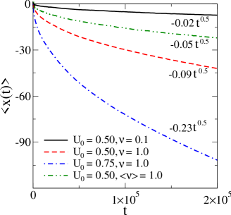
a)      b)

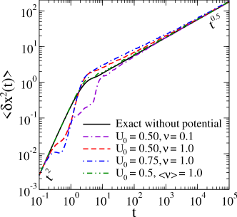
Figure 2: The mean particle position (a) and mean variance (b) at different values of the potential height $U_{0}$ and flashing frequency $\nu$ for periodic and random (green dash-dot-dot line) driving at $T=0.25$. The black line in (b) depicts exact analytical FLE result for the potential-free case.

Here black solid, red dash and blue dash-dot lines correspond to the periodic flashing, whereas green dash-dot-dot line relates to the random one. The direction of transport in figure 2(a) is negative and the transport has clearly subdiffusive character. We indicate in figure 2(a) also the corresponding power-law asymptotics. One can notice that stochastic flashing tends to delay the corresponding transport process in comparison with the periodic one of the same frequency (cf. red dash vs. green dash-dot-dot lines), and the transport becomes faster with the increased flashing frequency (this is but not a universal feature, see below). The diffusion is initially always ballistic (universal regime), $\langle\delta x^{2}(t)\rangle=v_{T}^{2}t^{2}$, where $v_{T}=\sqrt{k_{B}T/m}$ is thermal velocity. This is because the Brownian particle’s velocity is initially thermally distributed and the action of the medium requires some time to settle in. After some transient, subdiffusion follows asymptotically to one and the same universal dependence, $\langle\delta x^{2}(t)\rangle=2D_{\alpha}t^{\alpha}/\Gamma(1+\alpha)$ with $D_{\alpha}=k_{B}T/\eta_{\alpha}$, as in the absence of potential, independently of the potential height and the presence of driving, cf. in figure 2(b). This universality (or a weak sensitivity in the case of a strong fast driving [39]) is a benchmark of viscoelastic subdiffusion [22, 39, 53, 23]. We elaborate on this fact in more detail below.

4.1 Ergodicity

An important issue in anomalous transport is ergodicity [61, 62], i.e. whether time-average over a single particle trajectory delivers non-random result, same for all identical particles, or a principal randomness and scatter in the single-particle averages emerge. If this is the case, then the behavior and fate of each individual though identical particle is different, even in the limit of infinitely long trajectories, and only ensemble-averaging smears out this principal randomness and delivers non-random result. In the case of ergodic transport, a single-trajectory average should coincide with the result of the ensemble averaging. For example, CTRW subdiffusion with divergent mean residence times in traps is patently nonergodic [63] and single-trajectory averages obey some universal fluctuation laws [63, 64, 65, 66] leading to a universal scaling relating such transport and diffusion in periodic potentials [68]. On the contrary, viscoelastic subdiffusion, both free [67], and in time-independent potentials [22] was shown to be mostly ergodic, though some transient nonergodic features can be present. Whether it remains ergodic also in time-fluctuating fields presents a nontrivial problem. First, we checked the asymptotic ergodicity of ratchet viscoelastic transport which is expected. To show that this indeed is the case we plotted the fluctuating subvelocity $v_{\alpha}(t)$, obtained for a single trajectory as $v_{\alpha}(t)=\Gamma(1+\alpha)x(t)/t^{\alpha}$ in figure 3(a) vs. the ensemble-average obtained with $10^{4}$ particles. One can see that $v_{\alpha}(t)$ fluctuates around the ensemble average with the amplitude of fluctuations diminishing with $t$. In the limit $t\to\infty$ the both averages coincide and the transport is ergodic. For any finite $t$, statistical fluctuations are present, of course, also in ergodic case. Next, a single trajectory average of the squared displacement can be obtained as [64, 65, 67, 22],

$$\langle\delta x^{2}(t)\rangle_{\cal T}=\frac{1}{{\cal T}-t}\int_{0}^{{\cal T}-t}[x(t+t^{\prime})-x(t^{\prime})]^{2}dt^{\prime}.$$ (18)

In the ergodic case, this average should coincide in the limit ${\cal T}\to\infty$ but for any $t$ with the result of the ensemble averaging. If the agreement holds only for large $t$, then diffusion is asymptotically ergodic. For viscoelastic subdiffusion in fixed periodic potentials the agreement holds both for small $t$ (ballistic regime) and for large $t$ [22]. However, some deviations from ergodicity occur for intermediate $t$, on the time scale of diffusion over several potential periods. This is because even if the mean escape time exists the escape kinetics remains anomalous for activation barriers of an intermediate height [22].

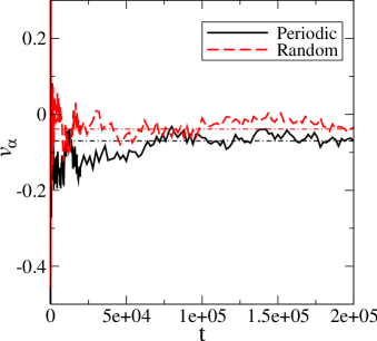
a)      b)

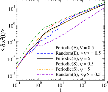
Figure 3: Subvelocity $v_{\alpha}(t)$, obtained for the single trajectory a) for periodic and random flashing ratchets at $U_{0}=0.5$, $T=0.25$ and linear frequency of flashing (its mean value) $\nu=0.5$. Mean deviation $\langle\delta x^{2}(t)\rangle$ b) for ensemble (E) and single trajectory (S) averaging at $U_{0}=0.5$ and $T=0.25$ for periodic and random flashing ratchets. The time averaging for a single trajectory is done using 16-exponential approximation to memory kernel and ${\cal T}=2\times 10^{7}$.

Diffusional spreading derived from single trajectories is compared with the corresponding ensemble averages in figure 3(b). In the ballistic regime, using $x(t+t^{\prime})-x(t^{\prime})\approx v(t^{\prime})t$ for small $t$ in Eq. (18), one obtains

$$\langle\delta x^{2}(t)\rangle_{\cal T}\approx t^{2}\frac{1}{{\cal T}-t}\int_{0}^{{\cal T}-t}v^{2}(t^{\prime})dt^{\prime}=\langle\delta v^{2}(t)\rangle_{\cal T}t^{2}.$$ (19)

Clearly, if in the limit ${\cal T}\to\infty$ the time average of $v^{2}(t)$ coincides with the ensemble average yielding $v_{T}^{2}$, then ergodicity holds also in the ballistic regime. In the absence of driving this is indeed the case [22]. However, a periodic driving exciting coherent oscillations emerging due to a combined action of the external trapping potential and the viscoelastic cage effect can cause large additional temporal fluctuations in $v(t)$ which are not self-averaged in $\langle v^{2}(t)\rangle_{\cal T}$. Accordingly, such a periodically driven subdiffusion ceases to be ergodic in the ballistic regime. Temporally but on a large intermediate time scale ergodicity is generally broken. Nevertheless, asymptotically it remains ergodic as figure 3(b) implies. Convergency to such asymptotically ergodic regime is very slow. However, it improves with the increased frequency of flashing, see the case $\nu=5$ in figure 3(b). For random driving, ergodicity in the discussed sense holds also in ballistic regime.

4.2 Frequency dependence

We proceed further with the dependence of anomalous current $v_{\alpha}$ on frequency $\nu$ at a fixed value of temperature for different potential amplitudes $U_{0}$. In the case of fluctuating tilt subdiffusive ratchets [39] this dependence was especially intriguing. That anomalous transport vanished in the limit of vanishing modulation frequency (adiabatic driving limit) and exhibited a maximum at intermediate frequencies. The origin of this maximum was related to stochastic resonance effect in Ref. [40]. This is in a sharp contrast with normal diffusion fluctuating tilt ratchets where transport optimizes namely in the adiabatic limit. The results for periodic flashing are shown in figure 4 and for stochastic driving in figure 5. For small driving frequencies subdiffusive transport occurs always in the natural negative direction, which is opposite to the natural positive direction of fluctuating tilt ratchet. Our anomalous Brownian motors share these features with their normal diffusion counterpart [1, 2].

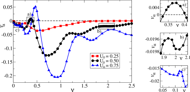
Figure 4: Anomalous current (subvelocity $v_{\alpha}$) as a function of linear frequency of periodic flashing at fixed temperature $T=0.25$ for different values $U_{0}$.

There are but novel features which are due to a profound role of the inertial effects in our model. We recall that in the used scaling the unit of time corresponds to a scaling time constant $\tau_{v}$ of the decay of velocity autocorrelation function. Correspondingly, the ballistic regime occurs until $t\sim 1$, when the potential is off. For periodic driving and a small potential height $U_{0}=0.25=T$ (see red line with squares in figure 4) subvelocity takes negative values for all flashing frequencies considered. The dependence of $|v_{\alpha}|$ on $\nu$ has a unique maximum at $\nu_{c0}\simeq 0.5$, where subdiffusive transport is optimized, with negative $v_{\alpha}$. For the fast-flashing regime, when $\nu>1$ subvelocity asymptotically decays to zero with $\nu$. Increase in the ratchet potential height $2U_{0}$ accompanied by an increased role of the inertial effects leads to a profound change in the character of the frequency-dependence $v_{\alpha}(\nu)$ (see black curve with circles for $U_{0}=0.5$ in figure 4). Let us study this dependence in more detail. The first difference from the former case is a multiple (double) current inversion, realized around $\nu_{c1}\simeq 0.335$ and $\nu_{c2}\simeq 0.402$. Enlarged picture of this inversion effect is shown in the insert $a)$ placed on the right panel in figure 4. Here, a well defined peak occurs at $\nu_{\max 1}=0.375$ with positive values for $\nu_{c1}<\nu<\nu_{c2}$. Furthermore, on the left side of $\nu<\nu_{c1}$ there is a maximum of $|v_{\alpha}|$ for negative $v_{\alpha}$. Increase of $\nu$ beyond $\nu_{c2}$ leads to a global maximum of $|v_{\alpha}|$ realized at $\nu_{\max 2}\simeq 0.75$. With a further increase in flashing frequency a complicated oscillatory pattern with several more relative minima and maxima in $|v_{\alpha}|$ emerges. With a further increase of the potential amplitude these oscillatory resonance-like features become more pronounced – compare two cases with $U_{0}=0.50$ and $U_{0}=0.75$ in figure 4. This is clearly related to an increased role of the inertial effects. First, the amplitude of oscillations in $v_{\alpha}(\nu)$ increases. Second, ever more extrema appear, see insets b) and c) in figure 4.

The situation is quite different in the case of random flashing. Dependencies of anomalous current versus mean linear frequency $\langle\nu\rangle$ at fixed temperature $T=0.25$ for different values of $U_{0}$ are shown in figure 5.

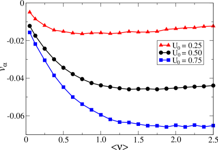
Figure 5: Anomalous current (subvelocity $v_{\alpha}$) as a function of mean linear frequency of random flashing at fixed temperature $T=0.25$ for different values $U_{0}$.

Here, contrary to the case of periodic flashing one has more simple dependencies $v_{\alpha}(\langle\nu\rangle)$ with one broad minimum for each considered potential amplitude $U_{0}$. Increase in $U_{0}$ leads to increase in absolute values for subvelocity, broadening the minimum and shifting minimum position towards larger values of mean linear frequency. Thus, in the random flashing case the system is not manifestly sensitive to inertial effects due to stochastic nature of flashing. The maximal value of subvelocity becomes also much smaller, compare figure 4 and figure 5, due to the absence of resonances.

A benchmark feature of viscoelastic subdiffusion is that it asymptotically does not depend on the presence of static periodic potential [22, 53, 23]. It was also only weakly dependent on driving in the case of rocking subdiffusive ratchets [39]. The diffusional spread in flashing ratchets is also practically not dependent on the potential amplitude $U_{0}$ and flashing frequency as figure 6 illustrates.

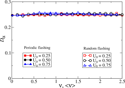
Figure 6: Sub-diffusion coefficient $D_{\alpha}$ as a function of linear frequency $\nu$ (or mean linear frequency $\langle\nu\rangle$) for periodic and random flashing, respectively, at fixed temperature $T=0.25$ and different values $U_{0}$.

One can see, that for both periodic and random flashing the anomalous diffusion coefficient does not display any profound dependence on the flashing frequency and the potential amplitude. It takes values around $0.25$, which is $D_{\alpha}=T$ in the scaled units, with a deviation which is less than 3% and lies within the statistical error margin of our simulations. Therefore, the corresponding generalized Peclet number ${\rm Pe}_{\alpha}:=v_{\alpha}/D_{\alpha}$, which measures the coherence and quality of transport, resembles the behavior of the absolute value of subcurrent in figures 4 and 5, which should be multiplied by factor 4 in order to obtain ${\rm Pe}_{\alpha}$.

4.3 Temperature dependence

The temperature dependence of subvelocity $v_{\alpha}$, and generalized Peclet number ${\rm Pe}_{\alpha}$ is mostly intriguing, whereas the dependence of subdiffusion coefficient $D_{\alpha}$ on temperature is expected to be trivial, $D_{\alpha}(T)=T$. We plotted numerical results for all these three quantities in figure 7 (periodic flashing) and figure 8 (stochastic flashing) for three different test values of the flashing frequency, $\nu=0.1$ (low-frequency), $\nu=0.375$ (intermediate frequency), and $\nu=0.75$ (high-frequency). The temperature dependencies of subvelocity share two common features, see figures 7(a) and 8(a). First, the subvelocity is finite in the limit $T\to 0$ (this is always so for random flashing, but only for certain frequency windows in the case of periodic flashing). Second, it diminishes to zero in the limit of high temperatures. The latter is expected, but the former is not, being highly surprising. Indeed, in a combination with the subdiffusion coefficient following to the expected linear dependence and vanishing in the limit $T\to 0$ [see figures 7(b) and 8(b)], the non-zero value of $v_{\alpha}$ in this limit means that the basic mechanism of operating our subdiffusive viscoelastic Brownian motors is very different from one in the case of normal Brownian motion. This is at odds with our expectations (see Introduction).

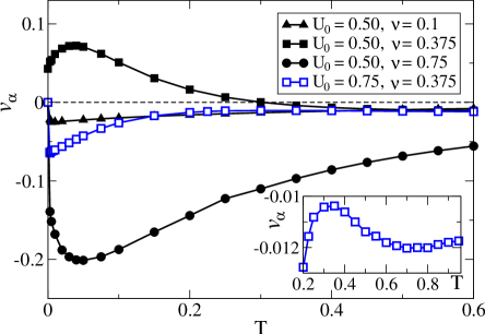
a)      b)
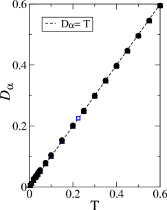
c)

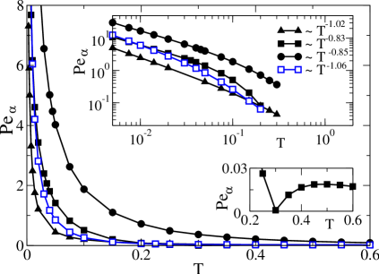
Figure 7: Anomalous current (subvelocity) $v_{\alpha}$ (a), subdiffusion coefficient $D_{\alpha}$ (b) and generalized Peclet number ${\rm Pe}_{\alpha}$ (c) versus temperature for the periodic flashing ratchets at different values for linear frequency of flashing $\nu$ and potential height $U_{0}$. The legend for (a), (b) and (c) figures is the same.

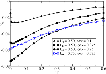
a)      b)
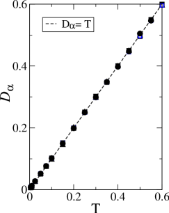
c)

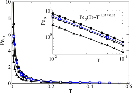
Figure 8: Anomalous current (subvelocity) $v_{\alpha}$ (a), subdiffusion coefficient $D_{\alpha}$ (b) and generalized Peclet number ${\rm Pe}_{\alpha}$ (c) versus temperature for the random flashing ratchets at different values for mean linear frequency of flashing $\langle\nu\rangle$ and potential height $U_{0}$. The legend for (a), (b) and (c) figures is the same.

Indeed, in the absence of viscoelastic effects the flashing Brownian motors of the studied kind are known to be essentially based on thermal diffusion, i.e. such transport is assisted by thermal fluctuations [9]. It is therefore expected to vanish in the limit $T\to 0$, where the thermal fluctuations vanish (in neglecting quantum effects). Our results say, however, that viscoelastic flashing ratchets are not based primarily on the thermal diffusion and thermal fluctuations. These are long-range elastic correlations which are at work here in combination with the potential fluctuations. Namely, the external field acting on the Brownian particle changes abruptly (on-off process) the energy stored in the elastic springs. Not only the Brownian particle moves under the influence of $f_{0}(x)$, but also the auxiliary particles under the influence of Brownian particle. Some of them rapidly adjust their positions, but there are also slow particles which cannot follow immediately. When the potential is off these extra sluggish particles pull the Brownian particle. This is why its motion is generally not frozen even at $T=0$ within our purely classical setup. Because subdiffusion diminishes with lowering temperature, the generalized Peclet number grows accordingly, ${\rm Pe}_{\alpha}(T)\sim 1/T^{\delta}$ with $\delta$ in the range $[0.83,1.05]$, see figure 7(c), and figure 8(c). Clearly, ${\rm Pe}_{\alpha}\to\infty$ in the limit $T\to 0$, where the transport becomes perfect.

There are also profound differences in the temperature-dependence of anomalous transport in the cases of periodic and random flashing. So, in the case of periodic flashing the transport can occur in the counterintuitive positive direction, see the curve for $U_{0}=0.5$, $\nu=0.375$ in figure 7(a). In this case, $v_{\alpha}$ remains finite also at $T=0$, and an inversion of the current direction with increasing temperature is possible. This is not so for other three curves in figure 7(a), where transport vanishes jump-like at $T=0$. Therefore, it seems obvious that for a periodic flashing there are frequency windows for permitted transport at $T=0$ (a detailed investigation of this issue is left for a separate study). On the contrary, for random driving in figure 8, a, the transport remained always finite at $T=0$. Moreover, here transport always occurs in the intuitive negative direction. Both in the random case and in the periodic case the transport can be optimized at some temperature $T_{\rm max}\neq 0$. It can be but also that $T_{\rm max}=0$.

5 Conclusions

With this work we put forward anomalously slow Brownian motors based on flushing subdiffusion in viscoelastic media. Both anomalous transport and subdiffusion were shown to be asymptotically ergodic. However, such driven subdiffusion can be transiently nonergodic on appreciably long time scales. The transport exhibits a remarkably good quality at low temperatures. It remains finite even at zero temperature in many cases (but not always in the case of periodic flashing) with zero dispersion. In this limit, the transport is clearly induced by long-range elastic correlations in a combination with potential flashing and not by the thermal noise of environment. This is surprising and at odds with a popular explanation of the origin of noise-induced flashing transport in the case memory-free stochastic dynamics [1, 2]. Moreover, in the case of periodic driving anomalous current exhibits multiple resonance-like features, can flow in the counter-intuitive direction, and invert its direction both with the change of flashing frequency and with change of temperature. The inertial cage effects are essential for many observed features. In particular, they are crucial for the resonance-like features manifested for high potential barriers in the case of periodic flashing. We hope that our research will stimulate further cross-fertilization of the field of fluctuation-induced transport and the field of anomalously slow transport and subdiffusion which flourish at present with little interaction. There emerges an increasing experimental support for the occurrence of subdiffusion in cytoplasm of biological cells and we believe that there might be also place for operating sluggish molecular motors of the kind described.

6 Acknowledgments

Support of this research by the Deutsche Forschungsgemeinschaft, Grant GO 2052/1-1 is gratefully acknowledged.

References

References

- [1] P. Reimann, Phys. Rep. 361, 57 (2002).
- [2] P. Hänggi and F. Marchesoni, Rev. Mod. Phys. 81, 387 (2009).
- [3] M. Switkes, C. M. Marcus, K. Campman, and A. C. Gossard, Science 283, 1905 (1999).
- [4] S. Denisov and S. Flach, Phys. Rev. E 64, 056236 (2001); H. Schanz, M. F. Otto, R. Ketzmerick, and T. Dittrich, Phys. Rev. Lett. 87, 070601 (2001).
- [5] T.L. Hill, Free Energy Transduction and Biochemical Cycle Kinetics (Dover, 2004)
- [6] T.Y. Tsong and R. D. Astumian, Prog. Biophys. Mol. Biol. 50, 1 (1987).
- [7] H. V. Westerhoff and Y. D. Chen, Proc. Natl. Acad. Sci. USA 82, 3222 (1985).
- [8] R. D. Astumian, Proc. Natl. Acad. Sci. USA 104, 19715 (2007).
- [9] P. Nelson, Biological Physics: Energy, Information, Life (W.H. Freeman, New York, 2004).
- [10] K. Kinosita (Jr.), R. Yasuda, H. Noji, S. Ishikawa, and M. Yoshida, Cell 93, 21 (1998).
- [11] S. Toyabe, T.Watanabe-Nakayama, T. Okamoto, S. Kudo, and E. Muneyuki, Proc. Natl. Acad. Sci. USA 108, 17951 (2011).
- [12] Yu. M. Romanovsky and A. N. Tikhonov, Physics-Uspekhi 53, 893 (2010).
- [13] A. Ajdari and J. Prost, CR Acad. Sci. Paris, Ser. II 315, 1635 (1992); R. D. Astumian and M. Bier, Phys. Rev. Lett. 72, 1766 (1994).
- [14] M. O. Magnasco, Phys. Rev. Lett. 71, 1477 (1993).
- [15] R. Bartussek, P. Hänggi, and J. G. Kissner, Europhys. Lett. 28, 459 (1994).
- [16] F. Jülicher, A. Ajdari, and J. Prost, Rev. Mod. Phys. 69, 1269 (1997).
- [17] J. C. Maxwell, Phil. Trans. R. Soc. Lond. 157, 49 (1867).
- [18] A. Gemant, Physics 7, 311 (1936).
- [19] T. G. Mason and D. A. Weitz, Phys. Rev. Lett. 74, 1250 (1995).
- [20] R. A. L. Jones, Soft Condensed Matter (Oxford University Press, Oxford, 2002).
- [21] T. A. Waigh, Rep. Prog. Phys. 68, 685 (2005).
- [22] I. Goychuk, Phys. Rev. E 80, 046125 (2009).
- [23] I. Goychuk, Adv. Chem. Phys. 150, 187 (2012).
- [24] R. Kubo, Rep. Prog. Phys. 29, 255 (1966).
- [25] R. Zwanzig, J. Stat. Phys. 9, 215(1973); R. Zwanzig, Nonequilibrium Statistical Mechanics (Oxford University Press, Oxford, 2001).
- [26] W. T. Coffey, Y. P. Kalmykov, J. T. Waldron, The Langevin Equation, 2nd ed. (World Scientific, Singapore, 2004).
- [27] U. Weiss, Quantum Dissipative Systems, 2nd ed. (World Scientific, Singapore, 1999).
- [28] S. A. Adelman, J. Chem. Phys. 64, 124 (1976).
- [29] P. Hänggi, H. Thomas, H. Grabert, P. Talkner, J. Stat. Phys. 18, 155 (1978).
- [30] P. Hänggi and F. Mojtabai, Phys. Rev. A 26, 1168 (1982).
- [31] J. T. Hynes, J. Phys. Chem. 90, 3701 (1986).
- [32] I. Goychuk and P. Hänggi, Phys. Rev. Lett. 99, 200601 (2007).
- [33] K. S. Cole and R. H. Cole, J. Chem. Phys. 9, 341 (1941).
- [34] I. Goychuk, Phys. Rev. E 76, 040102(R) (2007).
- [35] F. Amblard, et al., Phys. Rev. Lett. 77, 4470 (1996).
- [36] A. Caspi, R. Granek, and M. Elbaum, Phys. Rev. E 66, 011916 (2002).
- [37] G. Guigas, C. Kalla, and M. Weiss, Biophys. J. 93, 316 (2007).
- [38] J. Szymanski and M. Weiss, Phys. Rev. Lett. 103, 038102 (2009).
- [39] I. Goychuk, Chem. Phys. 375, 450 (2010).
- [40] I. Goychuk, V. Kharchenko, arXiv:1111.4833v1 [cond-mat.stat-mech] (2011).
- [41] G. Giacomo, et al., J. Stat. Mech. Theor. Exp. L12002 (2010).
- [42] T. Harms, R. Lipowsky, Phys. Rev. Lett. 79, 2895 (1997).
- [43] B. D. Hughes, Random walks and Random Environments, Vols. 1,2 (Clarendon Press, Oxford, 1995).
- [44] J.-P. Bouchaud and A. Georges, Phys. Rep. 195, 127 (1990).
- [45] R. Metzler and J. Klafter, Phys. Rep. 339, 1 (2000).
- [46] Fractional Dynamics: Recent Advances, eds. J. Klafter, S. C. Lim, R. Metzler (World Scientific, Singapore, 2011).
- [47] P. Hänggi and G.-L. Ingold, Chaos 15, 026105 (2005).
- [48] I. Goychuk and P. Hänggi, in: Stochastic Processes in Physics, Chemistry, and Biology, J. A. Freund, Th. Pöschel (eds.), Lect. Not. Phys. 557 (Springer, Berlin, 2000), pp. 7-20.
- [49] A. Isihara, Statistical Physics (Academic Press, New York, 1971).
- [50] B. B. Mandelbrot and J. W. van Ness, SIAM Rev. 10, 422 (1968).
- [51] E. Lutz, Phys. Rev. E 64, 051106 (2001).
- [52] S. Burov and E. Barkai, Phys. Rev. Lett. 100, 070601 (2008).
- [53] I. Goychuk and P. Hänggi, in: [46], Ch. 13, pp. 307-329.
- [54] F. Marchesoni and P. Grigolini, J. Chem. Phys. 78, 6287 (1983).
- [55] J.E. Straub, M. Borkovec, and B. J. Berne, J. Chem. Phys. 84, 1788 (1986).
- [56] R. G. Palmer, D. L. Stein, E. Abrahams, P. W. Anderson, Phys. Rev. Lett. 53, 958 (1984).
- [57] R. Kupferman, J. Stat. Phys. 114, 291 (2004).
- [58] P. Siegle, I. Goychuk, and P. Hänggi, Europhys. Lett. 93, 20002 (2011).
- [59] See on: http://www.nvidia.com/object/ cuda-home-new.html
- [60] B. Lindner, M. Kostur, and L. Schimansky-Geier, Fluct. Noise Lett. 1, R25 (2001).
- [61] A. M. Yaglom, An Introduction to the Theory of Stationary Random Functions (Dover, New York, 1972); see Sect. 1.4.
- [62] A. Papoulis, Probability, Random Variables, and Stochastic Processes (McGraw-Hill Book Company, New York, 1965); see Sect. 9-8., pp. 323-335.
- [63] G. Bel and E. Barkai, Phys. Rev. Lett. 94, 240602 (2005).
- [64] Y. He, S. Burov, R. Metzler and E. Barkai, Phys. Rev. Lett. 101, 058101 (2008).
- [65] A. Lubelski, I. M. Sokolov, and J. Klafter, Phys. Rev. Lett. 100, 250602 (2008).
- [66] I. M. Sokolov, E. Heinsalu, P. Hänggi, I. Goychuk, Europhys. Lett. 86, 30009 (2009).
- [67] W. H. Deng, E. Barkai, Phys. Rev. E 79, 011112 (2009).
- [68] I. Goychuk, E. Heinsalu, M. Patriarca, G. Schmid, P. Hänggi, Phys. Rev. E 73, R020101 (2006); E. Heinsalu, M. Patriarca, I. Goychuk, G. Schmid, P. Hänggi, Phys. Rev. E 73, 046133 (2006).