Vortex structures with complex points singularities in the two-dimensional  Euler  equation. New exact  solutions.

Abstract

In this work we found the new class of exact stationary solutions for 2D-Euler equations. Unlike of already known solutions, the new one contain complex singularities. We consider as complex, point singularities which have the vector field index greater than one. For example, the dipole singularity is complex because its index is equal to two. We present in explicit form a large class of exact localized stationary solutions for 2D-Euler equations with the singularity which index is equal to three. The obtained solutions are expressed in terms of elementary functions. These solutions represent complex singularity point surrounded by vortex satellites structure. We discuss also motion equation of singularities and conditions for singularity point stationarity which provides the stationarity of complex vortex configuration.

Anatoly TUR, Vladimir YANOVSKY^∗, Konstantin KULIK^∗

Université de Toulouse [UPS],
CNRS,Center d’Etude Spatiale des Rayonnements,
9 avenue du Colonel Roche, BP 4346,
31028 Toulouse Cedex 4, France. E-mail address: anatoly.tour@cesr.fr

^∗ Institute for Single Crystals, Nat. Academy of Science Ukraine,Kharkov 31001, Lenin Ave.60, s, Ukraine
E-mail address: yanovsky@isc.kharkov.ua, koskul@isc.kharkov.ua

keyword: 2D-Euler equations, exact solutions

PACS 05.45.-a,47.10.A-,47.10.-g,47.32.C-

Physica D: Nonlinear Phenomena, Volume 240, Issue 13, p. 1069-1079.

1
Introduction

The importance of exact solutions for 2D-Euler equations is well known. Today, the list of exact solutions is quite impressive. Without pretending to be exhaustive we will mention only some of them. First of all, this are classical solutions with smooth vorticity, such as Rankine and Kirchhoff type vortices (see, for example, the standard references [1]- [3] ), elliptical Moore and Suffman vortices.[2], Lamb dipole [1] and Stuart vortex pattern [4]. It is interesting, that these classical solutions are still topical (see for example recent works [5],[6]). The generalization of these solutions are the models of different coherent structures, vortex patches, and vortex crystals (see, for example, [7]-[13] and references therein), which are well observed in numerical and laboratory experiments (see, for example,[14]-[21]). Let us note that Stuart solution is based on the equation of Liouville type for stream function. Others classes of exact solutions rest upon the equation of Sinh-Poisson type for the stream function [22]- [24]. Some exact solutions in Lagrange coordinates are given on the work [25]. It should be noted the interesting class of Kida -Neu vortices [26],[27]. Also there is a lot of solutions with singular distribution of vorticity (see. [2] ), and solutions, which contain a smooth part of vorticity field as well as point singularities [28]- [32], which are usually forming symmetrical configurations.  Numerous publications deal with particular cases of point vortices (main references can be found in [2],[3],[33] and in works [34]- [38] ). It is known, that point vortices generate integrable dynamical systems as well as dynamical systems with chaotical behavior (see, for example,[3], [34], [37],[38] ). The case of a couple of point vortices, which vorticities are of same magnitude but opposite signs arouses particular interest. Such point vortices couples are usually called point dipoles. Many works are dedicated to the dynamics and statistic of point dipoles of this type (see, for example,[3],[36],[39]- [41].) Such point dipoles attract interest, especially in the theory of equations Charney-Hasegava-Mima for atmosphere and plasma. It means solutions of modon type [42] and its models obtained with the help of dipole structures (see, for example,[43]- [47]). Such a point dipole has two elliptical singular points (Fig.1). However, there are also 2D-point dipoles, which have different structure. They have one complex singular point which has the vector field index $\left|J\right|=2.$ This type of point dipoles appears naturally as a consequence of expansion of stream function $\Psi$ in multipoles moments, similar to usual electrodynamics. More precisely, we suppose, that the vorticity $\omega$ is localized in the restricted neighborhood $G$  of the  point $\overrightarrow{r}_{0}$, which belongs to 2D-plane. Let us denote the  characteristic scale of  domain $G$ by $a$, i.e.$\left\|G\right\|\lesssim a.$ Then the stream function $\Psi$:

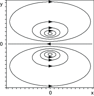
Figure 1: Couple of point vortices with vorticity of opposite signs, which is considered as point dipole.

$$\Psi(\overrightarrow{r},t)=-\frac{1}{4\pi}\int_{-\infty}^{+\infty}\omega(\overrightarrow{a},t)\ln\left|\overrightarrow{r}-\overrightarrow{a}\right|^{2}d\overrightarrow{a},$$ (1)

in the domain $\left|\overrightarrow{r}\right|\gg\left|\overrightarrow{a}\right|,$we can expand, as usual, in multipoles moments :

$$\Psi=-\frac{\Gamma_{0}}{2\pi}\ln\left|\overrightarrow{r}-\overrightarrow{r}_{0}\right|-\frac{1}{2\pi}\overrightarrow{D}\frac{\partial}{\partial\overrightarrow{x}}\ln\left|\overrightarrow{r}-\overrightarrow{r}_{0}\right|+\cdots$$ (2)

Here, the first term is obviously point vortex with the vorticity strength $\Gamma_{0}:\Gamma_{0}=\int\omega(\overrightarrow{a})d\overrightarrow{a}.$ The second term is the dipole $\Psi_{D}:$

$$\Psi_{D}=\frac{1}{2\pi}\frac{\overrightarrow{D}(\overrightarrow{r}-\overrightarrow{r}_{0})}{\left|\overrightarrow{x}-\overrightarrow{r}_{0}\right|^{2}},$$

with dipole moment $\overrightarrow{D}:\overrightarrow{D}=\int\omega(\overrightarrow{a})\overrightarrow{a}d\overrightarrow{a}.$ Further, we will call this dipole by dipole singularity to avoid any confusion with point dipole which is composed of two point vortices. It is easy to see the difference between them when calculating the vorticity. Apparently, the vorticity of vortices couple is proportional to the difference of two $\delta-$functions, whereas the vorticity of dipole singularity is proportional to derivative of $\delta-$function:

$$\omega\sim\delta^{{}^{\prime}}(x)=\underset{h\rightarrow 0}{\lim}\frac{1}{h}[\delta(x+h)-\delta(x)],$$

However, if the parameter $h$ is considered as minor, but final,

$$\omega\sim\frac{1}{h}[\delta(x+h)-\delta(x)],$$

then such a couple of closely located point vortices with the opposite vorticity may be considered as a approximative model of dipole singularity.

The important role of dipole singularities in dynamic of 2D-Euler equation was mentioned in the paper [48]. It is shown in this paper, that point dipole singularities are moving singularities of 2D- Euler equation which are forming together with point vortices the hamiltonian system of singulaties motion equation. This dynamical system has three independent integrals of motion in involution of Kirchhoff type. This fact means the complete integrability of the problem of motion of one dipole singularity and of one point vortex. Corresponding  exact solutions for the plane case without boundaries are given in the paper [49]. As it was noted earlier, the dipole singularity is more complex than point vortex since the index of its vector field is equal to two ( unlike simple singularities, which index is equal to $\pm 1$). In this paper we will continue the studies of solutions for 2D-Euler equation with complex singularities, which were started in [48], [49]. Also, we discuss in details some questions which previously were presented briefly. Further, we demonstrate, that more complex multipole singularities, generally speaking, are not compatible with the dynamic of 2D- Euler equation. But in this work we show that 2D-Euler equation has a new class of exact stationary solutions with complex singular point, which index is equal to three. These solutions are found in explicit form and expressed in terms of elementary functions. Obtained solutions describe localized vortex structures, in which complex singular point is surrounded by vortices satellites. In addition we discuss the equation of motion for singularities and we give the sufficient conditions of immobility for singular points; without this equation one can not guarantee the stationarity of solution.

2 Dipol singularities in 2D-Euler equation

We use 2D Euler equation in form of Poisson brackets for the vorticity $\omega$ and the stream function $\Psi:$

$$\omega=-\Delta\Psi$$ (3)

$$\frac{\partial\Delta\Psi}{\partial t}+\left\{\Delta\Psi,\Psi\right\}=0,$$ (4)

or in the form:

$$\frac{\partial\Delta\Psi}{\partial t}+V_{p}\frac{\partial\Delta\Psi}{\partial x_{p}}=\frac{d\Delta\Psi}{dt}=0.$$ (5)

here $\overrightarrow{V}$- is fluid velocity. Poisson brackets has the usual form:

$$\left\{A,B\right\}=\varepsilon_{ik}\frac{\partial A}{\partial x_{i}}\frac{\partial B}{\partial x_{k}}=\frac{\partial A}{\partial x}\frac{\partial B}{\partial y}-\frac{\partial A}{\partial y}\frac{\partial B}{\partial x}$$

$\varepsilon_{ik}-$is single anti symmetrical tensor:

$$\varepsilon_{12}=1,\varepsilon_{21}=-1,\varepsilon_{11}=\varepsilon_{22}=0;$$

$\overrightarrow{x}=(x,y)=(x_{1},x_{2}).$ Velocity field $\overrightarrow{V}=(V_{x},V_{y})=(V_{1},V_{2})$ is written in the form :

$$V_{i}=\varepsilon_{ik}\frac{\partial\Psi}{\partial x_{k}}.$$ (6)

As a stationary solutions for the Euler equation (4) one use often the anzatz:

$$\Delta\Psi=f(\Psi),$$ (7)

where $f(\Psi)$ is arbitrary enough differential function of $\Psi.$ For example, for the Lamb solution [1], $f(\Psi)$ is chosen as a linear function, for the Stuart solution [4] $f(\Psi)=\exp(-\Psi)$ and for solutions [22] $f(\Psi)=-\sinh\Psi$.

In solutions of type (7) the vorticity $\omega$ is smooth enough function. There are also stationary solutions in which the vorticity has a smooth part as well as one dimensional immobile singularities of point vortex type ( see, for example, [28]-[32] ).

In order to find stationary solutions for Euler equation (4) with singularities of point vortex type it was proposed in the work [32] the anzatz:

$$\Delta\Psi=f(\Psi)-\sum_{\alpha=1}^{N}\Gamma^{\alpha}\delta(\overrightarrow{x}-\overrightarrow{x}^{\alpha})$$

For the simplest case exact stationary solutions were found independently and in a different way in papers [31], [32]. In this work we study a more general anzatz. Let us suppose that the vorticity  $\omega=-\Delta\Psi$ can be presented in the form:

$$\Delta\Psi=f(\Psi)-\sum_{\alpha=1}^{N}\Gamma^{\alpha}\delta(\overrightarrow{x}-\overrightarrow{x}^{\alpha})-\sum_{\beta=1}^{M}D_{i}^{\beta}\frac{\partial}{\partial x_{i}}\delta(\overrightarrow{x}-\overrightarrow{x}^{\beta}).$$ (8)

In the expansion (8) the coordinates of singularities $\overrightarrow{x}^{\alpha},\overrightarrow{x}^{\beta}$ and coefficients $D_{i}^{\beta}$ may depend on time. Then it is supposed that vorticity is composed of smooth part and singular part as well, which is a generalized function. To begin, let us consider physical sense of development (8). First term in right part is obviously a smooth part of vorticity field. Second group of terms is vorticity, which is generated by the set of point vortices $N$, with stream function $\Psi_{N}$:

$$\Psi_{N}=-\frac{1}{4\pi}\sum_{\alpha=1}^{N}\Gamma^{\alpha}\ln\left|\overrightarrow{x}-\overrightarrow{x}^{\alpha}\right|^{2}.$$

The third group of terms in development (8) with first derivatives of $\delta$ - function describes the vorticity which is generated by group of  dipole singularities $M$:

$$\Delta\Psi_{M}=-\sum_{\beta=1}^{M}D_{i}^{\beta}\frac{\partial}{\partial x_{i}}\delta(\overrightarrow{x}-\overrightarrow{x}^{\beta}).$$

Actually, the let us apply the operator

$$D_{i}^{\beta}\frac{\partial}{\partial x_{i}}=D_{1}^{\beta}\frac{\partial}{\partial x_{1}}+D_{2}^{\beta}\frac{\partial}{\partial x_{2}}$$ (9)

to Laplace equation:

$$\frac{1}{4\pi}\Delta\ln\left|\overrightarrow{x}-\overrightarrow{x}^{\beta}\right|^{2}=\delta(\overrightarrow{x}-\overrightarrow{x}^{\beta})$$

It is obvious that:

$$\frac{1}{4\pi}\Delta\left(D_{i}^{\beta}\frac{\partial}{\partial x_{i}}\right)\ln\left|\overrightarrow{x}-\overrightarrow{x}^{\beta}\right|^{2}=\left(D_{i}^{\beta}\frac{\partial}{\partial x_{i}}\right)\delta(\overrightarrow{x}-\overrightarrow{x}^{\beta}).$$ (10)

That is why the vorticity which is generated by the third group of terms has the stream function $\Psi_{M}:$

$$\Psi_{M}=-\frac{1}{4\pi}\sum_{\beta=1}^{M}\left(D_{i}^{\beta}\frac{\partial}{\partial x_{i}}\right)\ln\left|\overrightarrow{x}-\overrightarrow{x}^{\beta}\right|^{2},$$ (11)

i.e.that is the sum $M$ stream functions of dipole singularities in the form:

$$\Psi_{D}^{\beta}=\frac{1}{2\pi}D_{i}^{\beta}\frac{(x_{i}-x_{i}^{\beta})}{\left|\overrightarrow{x}-\overrightarrow{x}_{\beta}\right|^{2}},$$ (12)

which are in the points $\overrightarrow{x}_{\beta}$ and have dipole moments $\frac{1}{2\pi}\overrightarrow{D}^{\beta}$. The velocity field of dipole singularity has evidently the form:

$$V_{x}^{D}=-\frac{\partial\Psi_{D}}{\partial y}=-\frac{1}{2\pi\left|\overrightarrow{x}-\overrightarrow{x}_{0}\right|^{2}}\left[D_{y}-\frac{2y(\overrightarrow{D}\overrightarrow{x})}{\left|\overrightarrow{x}-\overrightarrow{x}_{0}\right|^{2}}\right],$$

$$V_{y}^{D}=\frac{\partial\Psi_{D}}{\partial x}=\frac{1}{2\pi\left|\overrightarrow{x}-\overrightarrow{x}_{0}\right|^{2}}\left[D_{x}-\frac{2x(\overrightarrow{D}\overrightarrow{x})}{\left|\overrightarrow{x}-\overrightarrow{x}_{0}\right|^{2}}\right].$$

The presence of complementary sources of vorticity in form of derivatives of $\delta$ - function, itself, is not forbidden in (8), if they are compatible with Euler equation (4). We have to remind  that the singularity part of vorticity like every generalized function with point support is composed of $\delta-$ function sum and its derivatives only. However, in the next chapter we show that the condition of compatibility of development (8) with Euler equation is not trivial and engenders important restrictions for (8). Formulae which one needs to work with derivatives of generalized functions are well known, but for reader’s convenience we gave them in the Appendix.  Before studying the general expansion of vorticity (8) let us examine  some particular cases. We begin with trivial solution, which is describing  one point vortex. Let us remind, how from point of view of generalized functions theory, point vortex satisfies formally Euler equation. We will substitute vorticity and stream function of point vortex which are in point $\overrightarrow{x}_{0}=0,$ in Poisson brackets. Then we obtain:

$$\left\{\Psi,\Delta\Psi\right\}=\frac{\Gamma^{2}}{2\pi(x^{2}+y^{2})}[x\delta(x)]\delta^{{}^{\prime}}(y)-\frac{\Gamma^{2}}{2\pi(x^{2}+y^{2})}[y\delta(y)]\delta^{{}^{\prime}}(x)$$ (13)

This Poisson brackets is equal to zero since the terms in brackets are equal to zero from the generalized function theory point of view. The fact that Poisson brackets is equal to zero (13) is physically interpreted as absence of self-interaction in point vortex.If the Poisson bracket does not vanish for the solution with one singularity on the plane, then, typically, a self acceleration of this singularity appears . This effect is considered unacceptable from a physical point of view and the corresponding solutions must be rejected.

Let us examine in the same way one dipole singularity, which is in the point $\overrightarrow{x}_{0}$ and has the dipole moment $\overrightarrow{D}.$

The Poisson brackets (4) for one dipole singularity gets the form:

$$\left\{\Psi_{D},\Delta\Psi_{D}\right\}=\frac{\partial\Psi_{D}}{\partial x}\frac{\partial}{\partial y}\overrightarrow{D}\frac{\partial}{\partial\overrightarrow{x}}\delta(\overrightarrow{x}-\overrightarrow{x}_{0})-\frac{\partial\Psi_{D}}{\partial y}\frac{\partial}{\partial x}\overrightarrow{D}\frac{\partial}{\partial\overrightarrow{x}}\delta(\overrightarrow{x}-\overrightarrow{x}_{0}).$$ (14)

Let us show that Poisson brackets (14) is equal to zero. We substitute in (14) derivatives in explicit form and calculate it in details:

$$\frac{\partial}{\partial x}\overrightarrow{D}\frac{\partial}{\partial\overrightarrow{x}}\delta(\overrightarrow{x}-\overrightarrow{x}_{0})=D_{1}\delta_{xx}^{{}^{\prime\prime}}(x-x_{0})\delta(y-y_{0})+D_{2}\delta_{x}^{{}^{\prime}}(x-x_{0})\delta_{y}^{{}^{\prime}}(y-y_{0}),$$ (15)

$$\frac{\partial}{\partial y}\overrightarrow{D}\frac{\partial}{\partial\overrightarrow{x}}\delta(\overrightarrow{x}-\overrightarrow{x}_{0})=D_{1}\delta_{x}^{{}^{\prime}}(x-x_{0})\delta_{y}^{{}^{\prime}}(y-y_{0})+D_{2}\delta(x-x_{0})\delta_{yy}^{{}^{\prime\prime}}(y-y_{0}).$$ (16)

$$\frac{\partial\Psi_{D}}{\partial x}=\frac{1}{2\pi}\frac{D_{1}[(y-y_{0})^{2}-(x-x_{0})^{2}]-2D_{2}(x-x_{0})(y-y_{0})}{\left|\overrightarrow{x}-\overrightarrow{x}_{0}\right|^{4}},$$ (17)

$$\frac{\partial\Psi_{D}}{\partial y}=\frac{1}{2\pi}\frac{D_{2}[(x-x_{0})^{2}-(y-y_{0})^{2}]-2D_{1}(x-x_{0})(y-y_{0})}{\left|\overrightarrow{x}-\overrightarrow{x}_{0}\right|^{4}}.$$ (18)

As a result we obtain:

$$2\pi\left\{\Psi_{D},\Delta\Psi_{D}\right\}=\left[\frac{(D_{1}^{2}+D_{2}^{2})(y-y_{0})^{2}}{\left|\overrightarrow{x}-\overrightarrow{x}_{0}\right|^{4}}\delta_{y}^{{}^{\prime}}(y-y_{0})\right]\delta_{x}^{{}^{\prime}}(x-x_{0})-$$ (19)

$$-\left[\frac{(D_{1}^{2}+D_{2}^{2})(x-x_{0})^{2}}{\left|\overrightarrow{x}-\overrightarrow{x}_{0}\right|^{4}}\delta_{x}^{{}^{\prime}}(x-x_{0})\right]\delta_{y}^{{}^{\prime}}(y-y_{0})+$$

$$+\frac{D_{1}D_{2}[(y-y_{0})^{2}-(x-x_{0})^{2}]-2D_{2}^{2}(x-x_{0})(y-y_{0})}{\left|\overrightarrow{x}-\overrightarrow{x}_{0}\right|^{4}}\delta(x-x_{0})\delta_{yy}^{{}^{\prime\prime}}(y-y_{0})-$$

$$-\frac{D_{1}D_{2}[(x-x_{0})^{2}-(y-y_{0})^{2}]-2D_{1}^{2}(x-x_{0})(y-y_{0})}{\left|\overrightarrow{x}-\overrightarrow{x}_{0}\right|^{4}}\delta(y-y_{0})\delta_{xx}^{{}^{\prime\prime}}(x-x_{0}).$$

Let us use formulae from the Appendix. Action of first derivative of $\delta-$function on usual functions is given by formula (95). It follows from this formula that the first and second terms in formula (19) are zero, since they contain zeros of the following form:

$$(y-y_{0})\delta(y-y_{0});(y-y_{0})^{2}\mid_{y-y_{0}=0}\delta_{y}^{{}^{\prime}}(y-y_{0});$$

$$(x-x_{0})\delta(x-x_{0});(x-x_{0})^{2}\mid_{x-x_{0}=0}\delta_{x}^{{}^{\prime}}(x-x_{0}).$$

Besides, in third and fourth terms the term with the factor $D_{2}^{2},$ turns into zero because it contains zeros $(x-x_{0})\delta(x-x_{0})$, and the term with the factor $D_{1}^{2}$ turns into zero in the same way, because it contains zero $(y-y_{0})\delta(y-y_{0}).$ In addition, it is evident that the terms: $D_{1}D_{2}[(x-x_{0})^{2}\delta(x-x_{0})]\delta_{yy}^{{}^{\prime\prime}}(y-y_{0})$ and

$D_{1}D_{2}[(y-y_{0})^{2}\delta(y-y_{0})]\delta_{xx}^{{}^{\prime\prime}}(x-x_{0})$ are equal to zero. Consequently the brackets (19) is equal to:

$$2\pi\left\{\Psi_{D},\Delta\Psi_{D}\right\}=\frac{D_{1}D_{2}(y-y_{0})^{2}}{\left|\overrightarrow{x}-\overrightarrow{x}_{0}\right|^{4}}\delta(x-x_{0})\delta_{yy}^{{}^{\prime\prime}}(y-y_{0})-$$ (20)

$$-\frac{D_{1}D_{2}(x-x_{0})^{2}}{\left|\overrightarrow{x}-\overrightarrow{x}_{0}\right|^{4}}\delta(y-y_{0})\delta_{xx}^{{}^{\prime\prime}}(x-x_{0})$$

Now, for computing this equation we use the formula (97), which is needed to apply the second derivative of $\delta-$function in the commutator (20). It is obvious that all the terms turn into zero, excluding terms without derivatives of $\delta-$function, which are mutually eliminated:

$$2\pi\left\{\Psi_{D},\Delta\Psi_{D}\right\}=\frac{2D_{1}D_{2}}{\left|\overrightarrow{x}-\overrightarrow{x}_{0}\right|^{4}}\delta(\overrightarrow{x}-\overrightarrow{x}_{0})-\frac{2D_{1}D_{2}}{\left|\overrightarrow{x}-\overrightarrow{x}_{0}\right|^{4}}\delta(\overrightarrow{x}-\overrightarrow{x}_{0})=0.$$

Thereby we proved that there is no self-interaction in dipole singularity and, consequently, it is the exact stationary solution of Euler equation. We can also understand the absence of self-interaction in dipole singularity basing on simple physical considerations. Actually, from (Fig.2) one can see, that due to symmetry of stream line configuration, the flux of impulse which is flowing in singularity through arbitrary section $S$ is exactly equal to impulse flux which is flowing out from singularity through the same symmetrical section $S$. That means that the force which is acting on singularity is equal to zero and the singularity does not move.

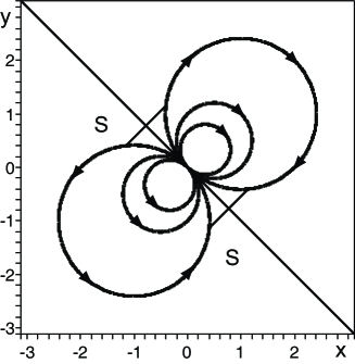
Figure 2: Dipole singularity with the index of vector field equal to 2.

Naturally the question arises: do the higher multipole singularities, for example, quadruple, self-interaction? To answer this question we have to calculate Poisson brackets $\left\{\Psi,\Delta\Psi\right\}$ for  quadruple singularity. The quadruple singularity has the stream function:

$$\Psi_{D_{2}}=-\frac{1}{8\pi}D_{i_{1}i_{2}}\frac{\partial^{2}}{\partial x_{i_{1}}\partial x_{i_{2}}}\ln\left|\overrightarrow{x}-\overrightarrow{x}_{0}\right|^{2},$$ (21)

and the vorticity:

$$\omega=\frac{1}{2}D_{i_{1}i_{2}}\frac{\partial^{2}}{\partial x_{i_{1}}\partial x_{i_{2}}}\delta(\overrightarrow{x}-\overrightarrow{x}_{0}).$$ (22)

When computing the Poisson brackets $\left\{\Psi,\Delta\Psi\right\}$ using the formula (98)  we obtain the following result:

$$\left\{\Psi_{D_{2}},\Delta\Psi_{D_{2}}\right\}=-\frac{1}{3\pi}\frac{D_{12}(D_{11}+D_{22})}{(x^{2}+y^{2})^{3}}\delta(\overrightarrow{x}),$$ (23)

which shows that there is self-interaction in the general case in quadruple singularity; (exception to the rule is special choice of coefficients: $D_{12}=0,$ or $D_{11}+D_{22}=0$). The self-interaction means that the given singularity is not physical. The similar result is obtained for multipoles of higher orders. Therefore, in general case the multipoles singularities of orders higher than dipole are not compatible with Euler equation.

3 Singularities motion and stationarity conditions.

According to the work [48] let us examine the question in which cases vorticity expansion (8) is compatible with Euler equation (4) and which restrictions arise from it  for stationary and not stationary cases. We consider singularities coordinates $\overrightarrow{x}_{\alpha},\overrightarrow{x}_{\beta}$ and all coefficients $\Gamma^{\alpha},D_{i}^{\beta}$ for general case as depending on time. Further, we will distinguish two cases: $f(\Psi)=0,f(\Psi)\neq 0.$ Let us first examine the first case $f(\Psi)=0.$ In this case the smooth part of vorticity is absent and the stream function $\Psi$ is determined by singularities only

$$\Psi=\Psi_{N}+\Psi_{M}$$ (24)

and derivatives of vorticity $\Delta\Psi$ obviously have the form :

$$\frac{\partial\Delta\Psi}{\partial t}=-\sum_{\alpha=1}^{N}\frac{d\Gamma^{\alpha}}{dt}\delta(\overrightarrow{x}-\overrightarrow{x}^{\alpha})+\sum_{\alpha=1}^{N}\Gamma^{\alpha}\frac{\partial\delta(\overrightarrow{x}-\overrightarrow{x}^{\alpha})}{\partial x_{i}}\frac{dx_{i}^{\alpha}}{dt}-$$ (25)

$$-\sum_{\beta=1}^{M}\frac{dD_{i}^{\beta}}{dt}\frac{\partial\delta(\overrightarrow{x}-\overrightarrow{x}^{\beta})}{\partial x_{i}}+\sum_{\beta=1}^{M}D_{i}^{\beta}\frac{\partial^{2}\delta(\overrightarrow{x}-\overrightarrow{x}^{\beta})}{\partial x_{i}\partial x_{k}}\frac{dx_{k}^{\beta}}{dt},$$

$$V_{p}\frac{\partial\Delta\Psi}{\partial x_{p}}=-V_{p}\sum_{\alpha=1}^{N}\Gamma^{\alpha}\frac{\partial\delta(\overrightarrow{x}-\overrightarrow{x}^{\alpha})}{\partial x_{p}}-V_{p}\sum_{\beta=1}^{M}D_{i}^{\beta}\frac{\partial^{2}\delta(\overrightarrow{x}-\overrightarrow{x}^{\beta})}{\partial x_{i}\partial x_{p}}.$$ (26)

Where $V_{p}$ - is fluid velocity (6), which can be written down in the following form:

$$V_{p}=-\frac{1}{4\pi}\varepsilon_{pq}\frac{\partial}{\partial x_{q}}\left[\sum_{\alpha=1}^{N}\Gamma^{\alpha}\ln\left|\overrightarrow{x}-\overrightarrow{x}^{\alpha}\right|^{2}+\sum_{\beta=1}^{M}(D_{i}^{\beta}\frac{\partial}{\partial x_{i}})\ln\left|\overrightarrow{x}-\overrightarrow{x}^{\beta}\right|^{2}\right].$$ (27)

We substitute (25) and (26) in Euler equation(5), and we obtain:

$$\sum_{\alpha=1}^{N}\left[\frac{d\Gamma^{\alpha}}{dt}\delta(\overrightarrow{x}-\overrightarrow{x}^{\alpha})-\Gamma^{\alpha}\frac{\partial\delta(\overrightarrow{x}-\overrightarrow{x}^{\alpha})}{\partial x_{i}}\frac{dx_{i}^{\alpha}}{dt}+V_{p}\Gamma^{\alpha}\frac{\partial\delta(\overrightarrow{x}-\overrightarrow{x}^{\alpha})}{\partial x_{p}}\right]+$$ (28)

$$+\sum_{\beta=1}^{M}\left[\frac{dD_{i}^{\beta}}{dt}\frac{\partial\delta(\overrightarrow{x}-\overrightarrow{x}^{\beta})}{\partial x_{i}}-D_{i}^{\beta}\frac{\partial^{2}\delta(\overrightarrow{x}-\overrightarrow{x}^{\beta})}{\partial x_{i}\partial x_{k}}\frac{dx_{k}^{\beta}}{dt}+V_{p}D_{i}^{\beta}\frac{\partial^{2}\delta(\overrightarrow{x}-\overrightarrow{x}^{\beta})}{\partial x_{i}\partial x_{p}}\right]=0.$$

Since equations for different singularities $\overrightarrow{x}^{\alpha}(t),\overrightarrow{x}^{\beta}(t)$ must go to zero independently, we obtain:

$$\sum_{\alpha=1}^{N}\left[\frac{d\Gamma^{\alpha}}{dt}\delta(\overrightarrow{x}-\overrightarrow{x}^{\alpha})-\Gamma^{\alpha}\frac{\partial\delta(\overrightarrow{x}-\overrightarrow{x}^{\alpha})}{\partial x_{i}}\frac{dx_{i}^{\alpha}}{dt}+V_{p}\Gamma^{\alpha}\frac{\partial\delta(\overrightarrow{x}-\overrightarrow{x}^{\alpha})}{\partial x_{p}}\right]=0,$$ (29)

$$\sum_{\beta=1}^{M}\left[\frac{dD_{i}^{\beta}}{dt}\frac{\partial\delta(\overrightarrow{x}-\overrightarrow{x}^{\beta})}{\partial x_{i}}-D_{i}^{\beta}\frac{\partial^{2}\delta(\overrightarrow{x}-\overrightarrow{x}^{\beta})}{\partial x_{i}\partial x_{k}}\frac{dx_{k}^{\beta}}{dt}+V_{p}D_{i}^{\beta}\frac{\partial^{2}\delta(\overrightarrow{x}-\overrightarrow{x}^{\beta})}{\partial x_{i}\partial x_{p}}\right]=0.$$ (30)

Every equation (29),(30) contains also singularities of different orders ($\delta-$functions and derivatives of $\delta-$ function). To satisfy each of equation (29), (30) the factors of singularities of different orders shall also go to zero independently. Let us begin with the simplest equation (29). The derivative of $\delta-$function acts on velocity field $\overrightarrow{V}$ according to formula (95). Because of non compressibility condition $\frac{\partial V_{p}}{\partial x_{p}}=0,$ the third term in formula (29) does not give additional contributions to singularities with $\delta-$functions. That is why when factors of $\delta-$functions are going to zero this gives the well known equation:

$$\frac{d\Gamma^{\alpha}}{dt}=0;\forall\alpha,$$

i.e. conservation of vorticity strength. Terms with the first derivatives from $\delta-$function give:

$$\sum_{\alpha=1}^{N}\Gamma^{\alpha}\left(\frac{dx_{p}^{\alpha}}{dt}-V_{p}\right)\frac{\partial\delta(\overrightarrow{x}-\overrightarrow{x}^{\alpha})}{\partial x_{p}}=0,$$ (31)

i.e. point vortices motion equations:

$$\left(\frac{dx_{p}^{\alpha}}{dt}-V_{p}\mid_{\overrightarrow{x}=\overrightarrow{x}^{\alpha}}\right)=0,(\alpha=1,2,...N)$$ (32)

(In equations (32) there are no terms with self-interaction). Let us examine now equations for point dipoles (30). The third term in equation (30) contains second derivatives from $\delta-$function. These derivatives act on velocity field $V_{p}(\overrightarrow{x},t)$ according to formula (97) in Appendix, and give the first ones and second ones as well. Since derivatives of different orders must be set equal to zero independently, the equation (30) splits into two groups of equations:

$$\sum_{\beta=1}^{M}\left(\frac{dD_{i}^{\beta}}{dt}-D_{i}^{\beta}\frac{\partial V_{p}}{\partial x_{i}}\mid_{\overrightarrow{x}=\overrightarrow{x}^{\beta}}\right)\frac{\partial\delta(\overrightarrow{x}-\overrightarrow{x}^{\beta})}{\partial x_{p}}=0,$$ (33)

$$\sum_{\beta=1}^{M}D_{i}^{\beta}\left(\frac{dx_{p}^{\beta}}{dt}-V_{p}\mid_{\overrightarrow{x}=\overrightarrow{x}^{\beta}}\right)\frac{\partial^{2}\delta(\overrightarrow{x}-\overrightarrow{x}^{\beta})}{\partial x_{i}\partial x_{p}}=0.$$ (34)

Equations (33),(34) are satisfied, if all factors of different singularities turn into zero independently and the number of equations coincides with the number of variables. Terms of point dipole with self-interaction as this was shown in previous chapter are absent. As a result we obtain motion equation of point dipoles:

$$\frac{dD_{i}^{\beta}}{dt}=D_{i}^{\beta}\frac{\partial V_{p}}{\partial x_{i}}\mid_{\overrightarrow{x}=\overrightarrow{x}^{\beta}},$$ (35)

$$\frac{dx_{p}^{\beta}}{dt}=V_{p}\mid_{\overrightarrow{x}=\overrightarrow{x}^{\beta}},(\beta=1,2,...M).$$ (36)

From (33),(34) follows that if all dipole moments are equal to zero, $(D_{i}^{\beta}=0,\forall\beta)$, then equations (33),(34) are absent and only the system of equation (32) remains for point vortices motion. And vice versa, one can see from equation (31) that if all $\Gamma^{\alpha}=0,\forall\alpha,$ then the system (31) is absent and only motion equations of point dipoles remain. For the general case the equation system (32),(35),(36), where the velocity has the form (27), describes motion of point vortices $N$ as well as motion of point dipoles $M$. This equation system was obtained for the first time in [48], where, in particular, was shown, that it can be written down in the Hamiltonian form. Further, to write down the equation system of singularities motion, we denote coordinates of point vortices as $x_{vi}^{\alpha}$ (where $\alpha-$ is the number of point vortex $\alpha=(1,2,...N)$ , index $i$ takes the values $i=1,2,$ i.e.denotes the coordinates of point vortex $x_{1}\equiv x,x_{2}\equiv y$,   the subscript $v$  means the vortex coordinates). In similar manner we denote the coordinates of dipole singularities as $x_{di}^{\beta}$ $($where $\beta-$is the number of dipole singularity $\beta=1,2,...M).$ Then, motion equation of singularities (32),(35),(36), taking into account formula (27) for fluid velocity, takes the form of :

$$\frac{dx_{vi}^{\alpha}}{dt}=-\varepsilon_{ik}\left[\sum\limits_{\gamma\neq\alpha}^{N}\frac{\Gamma_{\gamma}}{2\pi}\frac{(x_{vk}^{\alpha}-x_{vk}^{\gamma})}{\left|\overrightarrow{x}_{v}^{\alpha}-\overrightarrow{x}_{v}^{\gamma}\right|^{2}}+\right.$$ (37)

$$\left.+\sum\limits_{\beta=1}^{M}\frac{D_{l}^{\beta}}{\pi}\left(\frac{\delta_{lk}}{\left|\overrightarrow{x}_{v}^{\alpha}-\overrightarrow{x}_{d}^{\beta}\right|^{2}}-\frac{2(x_{vl}^{\alpha}-x_{dl}^{\beta})(x_{vk}^{\alpha}-x_{dk}^{\beta})}{\left|\overrightarrow{x}_{v}^{\alpha}-\overrightarrow{x}_{d}^{\beta}\right|^{4}}\right)\right]=0,$$

$$\frac{dx_{di}^{\beta}}{dt}=-\varepsilon_{ik}\left[\sum\limits_{\alpha=1}^{N}\frac{\Gamma_{\alpha}}{2\pi}\frac{(x_{dk}^{\beta}-x_{vk}^{\alpha})}{\left|\overrightarrow{x}_{v}^{\alpha}-\overrightarrow{x}_{d}^{\beta}\right|^{2}}+\right.$$ (38)

$$\left.+\sum\limits_{\gamma\neq\beta}^{M}\frac{D_{l}^{\gamma}}{\pi}\left(\frac{\delta_{lk}}{\left|\overrightarrow{x}_{d}^{\beta}-\overrightarrow{x}_{d}^{\gamma}\right|^{2}}-\frac{2(x_{dl}^{\beta}-x_{dl}^{\gamma})(x_{dk}^{\beta}-x_{dk}^{\gamma})}{\left|\overrightarrow{x}_{d}^{\beta}-\overrightarrow{x}_{d}^{\gamma}\right|^{4}}\right)\right],$$

$$\frac{dD_{i}^{\beta}}{dt}=D_{m}^{\beta}\varepsilon_{ik}\left[\sum\limits_{\alpha=1}^{N}\frac{\Gamma_{\alpha}}{2\pi}\left(\frac{\delta_{km}}{\left|\overrightarrow{x}_{d}^{\beta}-\overrightarrow{x}_{v}^{\alpha}\right|^{2}}-\frac{2(x_{dk}^{\beta}-x_{vk}^{\alpha})(x_{dm}^{\beta}-x_{vm}^{\alpha})}{\left|\overrightarrow{x}_{d}^{\beta}-\overrightarrow{x}_{d}^{\gamma}\right|^{4}}\right)+\right.$$ (39)

$$+\sum\limits_{\gamma\neq\beta}^{M}\frac{D_{l}^{\gamma}}{\pi}\left(-\frac{2\delta_{lk}(x_{dm}^{\beta}-x_{dm}^{\gamma})}{\left|\overrightarrow{x}_{d}^{\beta}-\overrightarrow{x}_{d}^{\gamma}\right|^{4}}-\frac{2\delta_{ml}(x_{dk}^{\beta}-x_{dk}^{\gamma})}{\left|\overrightarrow{x}_{d}^{\beta}-\overrightarrow{x}_{d}^{\gamma}\right|^{4}}-\right.$$

$$\left.\left.-\frac{2\delta_{mk}(x_{dl}^{\beta}-x_{dl}^{\gamma})}{\left|\overrightarrow{x}_{d}^{\beta}-\overrightarrow{x}_{d}^{\gamma}\right|^{4}}+\frac{8(x_{dl}^{\beta}-x_{dl}^{\gamma})(x_{dk}^{\beta}-x_{dk}^{\gamma})(x_{dm}^{\beta}-x_{dm}^{\gamma})}{\left|\overrightarrow{x}_{d}^{\beta}-\overrightarrow{x}_{d}^{\gamma}\right|^{6}}\right)\right].$$

Equations (37), (38) describe the motion of point vortices and dipole singularities as well and equation (39) describes time evolution of dipole moment. As this is shown in work [48] these equations have the Hamiltonian form:

$$\Gamma_{\alpha}\frac{dx_{vi}^{\alpha}}{dt}=\varepsilon_{ik}\frac{\partial H}{\partial x_{vk}^{\alpha}},$$ (40)

$$\frac{dx_{di}^{\beta}}{dt}=-\varepsilon_{ik}\frac{\partial H}{\partial D_{k}^{\beta}},$$

$$\frac{dD_{i}^{\beta}}{dt}=-\varepsilon_{ik}\frac{\partial H}{\partial x_{dk}^{\alpha}},$$

Here Hamiltonian $H$ has the form:

$$H=-\frac{1}{4\pi}\sum_{\begin{subarray}{c}\alpha=1,\beta=1\\ \alpha\neq\beta\end{subarray}}^{N}\Gamma_{\alpha}\Gamma_{\beta}\ln\left|\overrightarrow{x}_{v}^{\alpha}-\overrightarrow{x}_{v}^{\beta}\right|-\frac{1}{2\pi}\sum_{\alpha=1,\beta=1}^{\alpha=N,\beta=M}\frac{\Gamma_{\alpha}D_{l}^{\beta}(x_{vl}^{\alpha}-x_{dl}^{\beta})}{\left|\overrightarrow{x}_{v}^{\alpha}-\overrightarrow{x}_{d}^{\beta}\right|^{2}}-$$ (41)

$$-\sum_{\begin{subarray}{c}\beta\prec\gamma=1\\ \beta\neq\gamma\end{subarray}}^{M}\frac{2D_{m}^{\beta}(x_{dm}^{\beta}-x_{dm}^{\gamma})D_{l}^{\gamma}(x_{dl}^{\beta}-x_{dl}^{\gamma})-D_{m}^{\beta}D_{m}^{\gamma}(\overrightarrow{x}_{d}^{\beta}-\overrightarrow{x}_{d}^{\gamma})^{2}}{\pi\left|\overrightarrow{x}_{d}^{\beta}-\overrightarrow{x}_{d}^{\gamma}\right|^{4}}.$$

Equation system (40) has the conservation laws of the type of Kirchhoff’s generalized integrals i.e. the conservation laws related to motion equation invariance under translation and rotation of coordinates system:

$$I_{1}=\sum_{\alpha=1}^{N}\Gamma_{\alpha}x_{v1}^{\alpha}-\sum_{\beta=1}^{M}D_{1}^{\beta}=const.$$ (42)

$$I_{2}=\sum_{\alpha=1}^{N}\Gamma_{\alpha}x_{v2}^{\alpha}-\sum_{\beta=1}^{M}D_{2}^{\beta}=const.$$ (43)

$$J=\sum_{\alpha=1}^{N}\Gamma_{\alpha}(\overrightarrow{x}_{v}^{\alpha})^{2}-2\sum_{\beta=1}^{M}(\overrightarrow{D}^{\beta}\overrightarrow{x}_{d}^{\beta})=const.$$ (44)

As in case of point vortices there are three independent motion integrals in the involution: $H,J$ and $I_{1}^{2}+I_{2}^{2}$. This means that the motion of one vortex and one point dipole are integrable. The exact non stationary solutions for plane case without boundaries are given in [49]. Naturally, the question arises, is it possible or not to add for the non stationary case in expansion (8) more higher derivatives of $\delta$ - function, i.e.multipoles of higher order. Multipoles of higher order, than dipole produce two kinds of difficulties. First of all, as it was shown  in sectoin 2, that, generally speaking, singularities of this kind have self-interaction. From dynamical point of view, the substitution of high multipoles in Euler equation in accordance with the formula (96) Appendix A, engenders overdetermined equation system. Hence, for the non stationary case, vorticity expansion (8) is compatible with Euler equation with $f(\Psi)=0,$ if the following sufficient conditions are satisfied:

1.  Multipole moments starting from the quadruple one are equal to zero.

2.  Singularities motion obeys the equations (40).

Let us now examine stationary case, when $f(\Psi)\neq 0,\frac{df(\Psi)}{d\Psi}\neq 0.$ In this case the stream function can depend on time since singularities coordinates and dipoles moments are function on time. The substitution of vorticity (8) in Euler equation (5) gives for the smooth part of stream function the equation:

$$\left[\frac{\partial\Psi}{\partial t}+\sum_{\alpha=1}^{N}\left(\frac{\partial\Psi}{\partial x_{v}^{\alpha}}\frac{dx_{v}^{\alpha}}{dt}+\frac{\partial\Psi}{\partial y_{v}^{\alpha}}\frac{dy_{v}^{\alpha}}{dt}\right)+\sum_{\beta=1}^{M}\left(\frac{\partial\Psi}{\partial x_{d}^{\beta}}\frac{dx_{d}^{\beta}}{dt}+\frac{\partial\Psi}{\partial y_{d}^{\beta}}\frac{dy_{d}^{\beta}}{dt}\right)+\right.$$ (45)

$$\left.+\sum_{\beta=1}^{M}\frac{\partial\Psi}{\partial D_{i}^{\beta}}\frac{dD_{i}^{\beta}}{dt}\right]\frac{df(\Psi)}{d\Psi}=0.$$

The first term is related to explicit dependence of stream function $\Psi$ on time, the second one and the third one are related to singularities motion. The fourth term in (45) is related to dependence of dipole moments on time. We have to add to the equation (45) equations for singularities parts of vorticity field which were already given (formulae (40)). In the case $\frac{df(\Psi)}{d\Psi}=0,$ the equation (45) is absent and only singularities motion equations remain. The sufficient condition of stationarity, i.e. the (45) goes to zero when $\frac{df(\Psi)}{d\Psi}\neq 0$ consists in the following:

1.  Stream function does not depend explicitly on time.

2.  All singularities do not move.

3.  All dipole moments $D_{i}^{\beta}$ are not function of time.

All terms which contain the velocity $V_{p}$ in equation (28) form obviously the Poisson brackets $\{\Psi,\Delta\Psi\}$. That is why the sufficient condition of immobility for all singularities  and of stationarity for all dipole moments is the condition when Poisson brackets goes to zero:

$$\{\Psi,\Delta\Psi\}=0,$$ (46)

This means that all factors of all independent singularities in Poisson brackets go to zero (46).

4 Exact stationary solutions with complex singularities

Now we consider the problem of exact stationary solutions of 2D-Euler equation, when $\frac{df(\Psi)}{d\Psi}\neq 0.$ Further, it is easy to consider the Poisson brackets

$$\frac{\partial\Psi}{\partial x}\frac{\partial\Delta\Psi}{\partial y}-\frac{\partial\Psi}{\partial y}\frac{\partial\Delta\Psi}{\partial x}=0$$ (47)

as dimensionless. Let us choose the anzatz (8) in the form:

$$\Delta\Psi=\exp\left(-\frac{\Psi}{\Gamma_{0}}\right)+4\pi n\Gamma_{0}\delta(\overrightarrow{x}-\overrightarrow{x}_{0})-4\pi\overrightarrow{D}\frac{\partial}{\partial\overrightarrow{x}}\delta(\overrightarrow{x}-\overrightarrow{x}_{0})$$ (48)

when function $f(\Psi)$ is chosen in the same way as in the Stuart work [4] ; we suppose that coefficients $\Gamma$ and $\overrightarrow{D}$ are constant, and the coordinate $\overrightarrow{x}_{0}$ is not depending on time. (For the sake of simplicity we can choose $\overrightarrow{x}_{0}=0$). $n-$ is positive integer number. By means of evident rescaling:

$$\frac{\Psi}{\Gamma_{0}}\rightarrow\Psi^{{}^{\prime}},x\rightarrow\Gamma_{0}^{\frac{1}{2}}x^{{}^{\prime}},y\rightarrow\Gamma_{0}^{\frac{1}{2}}y^{{}^{\prime}},\frac{\overrightarrow{D}}{\Gamma_{0}^{\frac{3}{2}}}\rightarrow\overrightarrow{D}^{{}^{\prime}}.$$ (49)

equation (48) is reduced to the more simple equation (the primes were omitted):

$$\Delta\Psi=\exp(-\Psi)+4\pi n\delta(\overrightarrow{x})-4\pi\overrightarrow{D}\frac{\partial}{\partial\overrightarrow{x}}\delta(\overrightarrow{x}).$$ (50)

(Let us note, that when $\overrightarrow{D}\equiv$0 the equation (50) has the solutions found in [31],[32]). First of all, let us find exact solutions for the equation (50), and then we prove, that they are exact stationary solutions of 2D-Euler equation (47). Now we can look for the solutions of equation (50) in the Liouville form:

$$\Psi=-\ln 8\frac{\left|u^{{}^{\prime}}(z)\right|^{2}}{(1+\left|u(z)\right|^{2})^{2}}.$$ (51)

when $u^{{}^{\prime}}(z)=\frac{du(z)}{dz},$ is the unknown for the moment function of complex variable $z=x+iy$ and $u(z)-$ is primitive function.

Direct calculation of $\Delta\Psi$ (51) gives:

$$\Delta\Psi=8\frac{\left|u^{{}^{\prime}}(z)\right|^{2}}{(1+\left|u(z)\right|^{2})^{2}}-\Delta\ln\left|u^{{}^{\prime}}(z)\right|^{2}.$$ (52)

it is important to note that the formula (52) is valid for arbitrary analytical function $u^{{}^{\prime}}(z)$ independently of its singularities structure.

We substitute the formula (52) into equation (50) and obtain the equation for the function $\left|u^{{}^{\prime}}(z)\right|^{2}:$

$$-\Delta\ln\left|u^{{}^{\prime}}(z)\right|^{2}=4\pi n\delta(\overrightarrow{x})-4\pi\overrightarrow{D}\frac{\partial}{\partial\overrightarrow{x}}\delta(\overrightarrow{x}).$$ (53)

It is easy to see that the equation (53) is satisfied, if we choose the function $\left|u^{{}^{\prime}}(z)\right|^{2}$ in the form:

$$\left|u^{{}^{\prime}}(z)\right|^{2}=\frac{1}{\left|z\right|^{2n}}\exp\overrightarrow{D}\frac{\partial}{\partial\overrightarrow{x}}\ln\left|z\right|^{2}.$$ (54)

Indeed:

$$\ln\left|u^{{}^{\prime}}(z)\right|^{2}=-n\ln\left|z\right|^{2}+\overrightarrow{D}\frac{\partial}{\partial\overrightarrow{x}}\ln\left|z\right|^{2}.$$ (55)

The first term in (55) gives the Green function of Laplace equation:

$$\Delta\ln\left|z\right|^{2}=4\pi\delta(\overrightarrow{x})$$ (56)

and describes the point vortex. The second term in (55) is a result of application of the operator $\overrightarrow{D}\frac{\partial}{\partial\overrightarrow{x}}$ to the equation (56) and describes the point dipole. Let us introduce the complex dipole moment :

$$D=D_{1}+iD_{2}.$$ (57)

Then the dipole operator $\overrightarrow{D}\frac{\partial}{\partial\overrightarrow{x}}$ can be written in the complex form:

$$\overrightarrow{D}\frac{\partial}{\partial\overrightarrow{x}}=D\frac{\partial}{\partial z}+\overline{D}\frac{\partial}{\partial\overline{z}}.$$ (58)

(When $\overline{D},\overline{z}$ - denote complex conjugated values).

The function (54) can be written down in the form:

$$\left|u^{{}^{\prime}}(z)\right|^{2}=\frac{1}{\left|z\right|^{2n}}\exp\left(D\frac{\partial}{\partial z}+\overline{D}\frac{\partial}{\partial\overline{z}}\right)(\ln z+\ln\overline{z})=\frac{1}{z^{n}}\exp\left(\frac{D}{z}\right)\frac{1}{\overline{z}^{n}}\exp\left(\frac{\overline{D}}{\overline{z}}\right).$$ (59)

From formula (59) follows, that functions $u^{{}^{\prime}}(z)$ can be chosen in the form:

$$u^{{}^{\prime}}(z)=\frac{1}{z^{n}}\exp\left(\frac{D}{z}\right).$$ (60)

In the point $z=0$, the function $u^{{}^{\prime}}(z)$ (60) has essential singular point, which joins the pole of order $n.$ Now let us find the primitive function $u_{n}(z):$

$$u_{n}(z)=\int\exp\left(\frac{D}{z}\right)\frac{dz}{z^{n}}.$$ (61)

Using the new variable $w=\frac{D}{z}$, we obtain:

$$u_{n}(w)=-\frac{1}{D^{n-1}}\int W^{(n-2)}\exp WdW.$$ (62)

From the formula (62) we can see that the primitive function is elementary function only with $n\geq 2.$ This particular case is examined in this work (others cases will be considered separately).

Integration by parts in the formula (62) with $n\geq 2$, gives:

$$u_{n}(z)=-\frac{1}{Dz^{n-2}}\exp\left(\frac{D}{z}\right)P_{n-2}(z);$$ (63)

where the polynomial $P_{n-2}(z)$ has the form:

$$P_{n-2}(z) = 1-(n-2)(\frac{z}{D})+(n-2)(n-3)\left(\frac{z}{D}\right)^{2}+\cdots$$

$$+(-1)^{n-3}(n-2)!\left(\frac{z}{D}\right)^{n-3}+(-1)^{n-2}(n-2)!\left(\frac{z}{D}\right)^{n-2}.$$

As a result, $\left|u_{n}(z)\right|^{2}$ has the form:

$$\left|u_{n}(z)\right|^{2}=\frac{1}{\left|D\right|^{2}\left|z\right|^{2(n-2)}}\exp\left(2\frac{D_{1}x+D_{2}y}{x^{2}+y^{2}}\right)\left|P_{n-2}(z)\right|^{2}.$$ (65)

The primitive function $u_{n}(z)$ (63), like the function $u^{{}^{\prime}}(z)$ (60) has in $z=0$ the essential singular point, which joins the pole of order $(n-2).$ In the real form $\left|u^{{}^{\prime}}(z)\right|^{2}$, has obviously the following form:

$$\left|u^{{}^{\prime}}(z)\right|^{2}=\frac{1}{(x^{2}+y^{2})^{n}}\exp\left(2\frac{D_{1}x+D_{2}y}{x^{2}+y^{2}}\right).$$ (66)

Consequently, the essential singular point describes in the complex form the singularities of point dipole kind, while the pole describes the point vortex, since the expression (66) generates following terms in stream function (51):

$$-\ln\left|u^{{}^{\prime}}(z)\right|^{2}=n\ln(x^{2}+y^{2})-2\frac{D_{1}x+D_{2}y}{x^{2}+y^{2}}.$$

Hence, the exact solution of the equation (50) is given by the formula (51), where $u(z)$ is defined by the expression (63), while $u^{{}^{\prime}}(z)-$ by the formula (60). Now we can prove, that the obtained solution turns into zero the Poisson brackets (47). At first, let us calculate the velocity field. Derivatives $\frac{\partial\Psi}{\partial x}$ and $\frac{\partial\Psi}{\partial y}$ have the form:

$$\frac{\partial\Psi}{\partial x}=\frac{2}{1+\left|u(z)\right|^{2}}\frac{\partial}{\partial x}u(z)\overline{u(z)},$$

$$\frac{\partial\Psi}{\partial y}=\frac{2}{1+\left|u(z)\right|^{2}}\frac{\partial}{\partial y}u(z)\overline{u(z)}.$$

Using the formulae:

$$\frac{\partial}{\partial x}=\frac{\partial}{\partial z}+\frac{\partial}{\partial\overline{z}},\ \ \ \ \frac{\partial}{\partial y}=i\left(\frac{\partial}{\partial z}-\frac{\partial}{\partial\overline{z}}\right),$$

we obtain a more convenient formula for derivatives:

$$\frac{\partial\Psi}{\partial x}=\frac{2}{1+\left|u(z)\right|^{2}}\left(\overline{u}\frac{du}{dz}+u\overline{\frac{du}{dz}}\right),$$

$$\frac{\partial\Psi}{\partial y}=\frac{2i}{1+\left|u(z)\right|^{2}}\left(\overline{u}\frac{du}{dz}-u\overline{\frac{du}{dz}}\right).$$

Taking into account the formula (60), after simple algebraic transformations we obtain the expression for components of velocity field:

$$\frac{\partial\Psi}{\partial x}=-\frac{2\exp\left(\frac{D\overline{z}+\overline{D}z}{\left|z\right|^{2}}\right)}{(1+\left|u(z)\right|^{2})\left|D\right|^{2}\left|z\right|^{2n}}(D\overline{z}^{2}\overline{P}_{n-2}+\overline{D}z^{2}P_{n-2}),$$ (67)

$$\frac{\partial\Psi}{\partial y}=-\frac{2i\exp\left(\frac{D\overline{z}+\overline{D}z}{\left|z\right|^{2}}\right)}{(1+\left|u(z)\right|^{2})\left|D\right|^{2}\left|z\right|^{2n}}(D\overline{z}^{2}\overline{P}_{n-2}-\overline{D}z^{2}P_{n-2}).$$ (68)

(Let us remind, that $n\geq 2$). Now we show that function (51),(63) is an exact solution of Poisson brackets (47). For that we substitute the expression for vorticity (48) and derivatives (67), (68) into Poisson brackets (47). First of all we examine the simplest case $n=2.$ In this case the polynomial $P_{n-2}=1$ and derivatives (67), (68) take the simple form:

$$\frac{\partial\Psi}{\partial x}=-\frac{4\exp\left(\frac{D\overline{z}+\overline{D}z}{\left|z\right|^{2}}\right)}{(1+\left|u\right|^{2})\left|D\right|^{2}\left|z\right|^{4}}(D_{1}x^{2}+2D_{2}xy-D_{1}y^{2}),$$ (69)

$$\frac{\partial\Psi}{\partial y}=\frac{4\exp\left(\frac{D\overline{z}+\overline{D}z}{\left|z\right|^{2}}\right)}{(1+\left|u\right|^{2})\left|D\right|^{2}\left|z\right|^{4}}(D_{2}x^{2}-2D_{1}xy-D_{2}y^{2}),$$ (70)

$$\left|u(z)\right|^{2}=\frac{1}{\left|D\right|^{2}}\exp\left(\frac{D\overline{z}+\overline{D}z}{\left|z\right|^{2}}\right).$$ (71)

We write the Poisson brackets (47) in the explicit form:

$$\{\Psi,\Delta\Psi\}=4\pi n\left[\frac{\partial\Psi}{\partial x}\delta(x)\delta^{{}^{\prime}}(y)-\frac{\partial\Psi}{\partial y}\delta(y)\delta^{{}^{\prime}}(x)\right]-$$ (72)

$$-4\pi\left[D_{1}\frac{\partial\Psi}{\partial x}-D_{2}\frac{\partial\Psi}{\partial y}\right]\delta^{{}^{\prime}}(x)\delta^{{}^{\prime}}(y)-$$

$$-4\pi\left[D_{2}\frac{\partial\Psi}{\partial x}\delta(x)\delta^{{}^{\prime\prime}}(y)-D_{1}\frac{\partial\Psi}{\partial y}\delta(y)\delta^{{}^{\prime\prime}}(x)\right].$$

It is obvious, that all the terms in the first brackets (72) are equal to zero because they contain this kind of zeros:

$$x^{2}\delta(x),x\delta(x),x^{2}\delta^{{}^{\prime}}(x);\ \ \ \ \ y^{2}\delta(y),y\delta(y),y^{2}\delta^{{}^{\prime}}(y).$$

In the second brackets one part of terms is also equal to zero, but there are dangerous terms of this type: $xy\delta^{{}^{\prime}}(x)\delta^{{}^{\prime}}(y).$ However, these terms are part of second brackets in the following combination:

$$\left(D_{1}\frac{\partial\Psi}{\partial x}-D_{2}\frac{\partial\Psi}{\partial y}\right)\delta^{{}^{\prime}}(x)\delta^{{}^{\prime}}(y)=[\cdots](-D_{1}D_{2}xy+D_{2}D_{1}xy)\delta^{{}^{\prime}}(x)\delta^{{}^{\prime}}(y)=0,$$

i.e. are reciprocally cancelled. (Here brackets $[\cdots]$ denote the common factor). Now we consider the last brackets in (72). In this brackets also, one part of terms turns into zero at once, but there are dangerous terms of this kind: $y^{2}\delta(x)\delta^{{}^{\prime\prime}}(y)$ and $x^{2}\delta(y)\delta^{{}^{\prime\prime}}(x)$. These dangerous terms are part of the brackets (72) in the following combination:

$$[\cdots][D_{2}D_{1}y^{2}\delta(x)\delta^{{}^{\prime\prime}}(y)-D_{1}D_{2}x^{2}\delta(y)\delta^{{}^{\prime\prime}}(x)]$$ (73)

(Here brackets $[\cdots]$ denote the common factor). Now we use the formula (97). From this formula one can see, that dangerous terms have the form:

$$D_{1}D_{2}\delta(x)\delta(y)\frac{d^{2}}{dy^{2}}y^{2}-D_{1}D_{2}\delta(x)\delta(y)\frac{d^{2}}{dx^{2}}x^{2}=0$$ (74)

and are cancelled in commutator (72). Others terms are obviously zero. Consequently, the Poisson brackets turn into zero for all singularities.  According to the results of chapter 3, this guarantees that singularities do not move and that the dipole moment $\overrightarrow{D}$ is conserved. It is proved that the obtained solution of equation (50), is exact, stationary solution of 2D-Euler equation (47) with $n=2.$ let us consider now the general case $n\succ 2.$ In this case velocities (67), (68) contain the polynomials $P_{n-2}(z)$ i $\overline{P_{n-2}}(z)$ (4).

It is  clear now that the additional powers $z$ or $\overline{z}$ in these polynomials generate in Poisson brackets zero terms only. The dangerous terms coincide only with the first term in the polynomial $P_{n-2}(z)$, i.e. unit. But these  terms correspond to the case $n=2$ , and are already been considered. Hence, we prove that formulae in (51), together with the function $u_{n}(z)$ (63), give exact stationary solution of 2D-Euler equation with $n\geq 2.$ In explicit form this solution has the form :

$$\Psi=-\ln 8-\ln\left|u^{{}^{\prime}}(z)\right|^{2}+2\ln(1+\left|u(z)\right|^{2})=$$ (75)

$$=-\ln 8+n\ln(x^{2}+y^{2})-2\frac{D_{1}x+D_{2}y}{x^{2}+y^{2}}+$$

$$+2\ln\left[1+\frac{\left|P_{n-2}(z)\right|^{2}}{\left|D\right|^{2}(x^{2}+y^{2})^{(n-2)}}\exp\left(2\frac{D_{1}x+D_{2}y}{x^{2}+y^{2}}\right)\right].$$

From equation (75) it follows that the essential singularity splits up into singularities of point vortex and point dipoles types. However, as we will see later, the fusion of these singularities leads to a singular point with more complex geometry with a vector field index equal to three. This can be interpreted as the sum of the indexes of the point vortex and the point dipole.

5 Examples of vortex structures with complex singularities

1) First of all let us examine the simplest case, when $n=2.$ In this case the function $u_{2}(z)$ (63) has the form:

$$u_{2}(z)=-\frac{1}{D}\exp\left(\frac{D}{z}\right),$$ (76)

The function $\left|u_{2}(z)\right|^{2}$ is given by (71), $u_{2}^{{}^{\prime}}(z)$ has the form:

$$\left|u_{2}^{{}^{\prime}}(z)\right|^{2}=(x^{2}+y^{2})^{-2}\exp\left(2\frac{D_{1}x+D_{2}y}{x^{2}+y^{2}}\right).$$ (77)

As a result we find the stream function (51):

$$\Psi=-\ln 8+2\ln(x^{2}+y^{2})-2\frac{D_{1}x+D_{2}y}{x^{2}+y^{2}}+$$ (78)

$$+2\ln\left[1+\frac{1}{D_{1}^{2}+D_{2}^{2}}\exp\left(2\frac{D_{1}x+D_{2}y}{x^{2}+y^{2}}\right)\right]$$

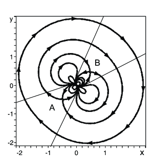
Figure 3: The simplest vortex structure with the index of vector field equal to 3 (n=2). Complex singularity is a result of the fusion of essential singular point (dipole singularity) with the pole (point vortex). One can see the presence of two hyperbolic points A and B, external and internal correspondingly. Separatrix of these points connect these hyperbolic points with the central complex singular point. Straight lines indicate exceptional directions of central singular point.

Farther, we can consider that $D_{1}=D_{2}.$ The vortex structure which is described by the stream function (78), is presented on (Fig.3), with $D_{1}=D_{2}=1.$ It is clear, that with great values $\left|\overrightarrow{x}\right|^{2}\rightarrow\infty,$ the stream function (78) coincides asymptotically with the stream function of point vortex with negative vorticity. From (Fig.3) one can see that inside of external closed stream line there is a vortex structure with the a non trivial topology of stream line. In the center there is a complex singular point, which results from the coincidence of singularities of point vortex and point dipole types. Furthermore, one can see the presence of two hyperbolic points, one outside $A$ and another inside $B$ . Separatrix of these points link the hyperbolic points with the central complex singular point. We examine more in details the structure of complex singular point. The general theory of such kind of singularities is stated in qualitative theory of ordinary differential equations (see, for example, [50], [51] ). According to this theory, first of all, we need to choose exceptional directions of the singular point. This are directions of tangents, following which the infinite number of integral curves go inside of the singular point and outside of it. One can see from (Fig.3), that there are four such exceptional directions which are designated on (Fig.3) by direct lines. Integral curves which are inside of exceptional lines form sectors. In our case, between the lines there are only four elliptical sectors (see, for example, [51] ). According to the general theory, the index $J(0)$ of complex singular point is given by Bendixson’s formula (see, for example, [50]):

$$J(0)=\frac{1}{2}(2+n_{e}-n_{h}),$$ (79)

where $n_{e}-$ is the number of elliptic sectors and $n_{h}-$ is the number of hyperbolic sectors. In our case $n_{h}=0,n_{e}=4.$ That is why

$$J(0)=3.$$ (80)

The condition (80) means, that the complex singular point is structurally stable, because the necessary and sufficient condition of the structural stability for complex singular point on plane is, that its index $J(0)\neq 0.$ (see, for example, [51]). Note, that in case of dipole singularity exceptional directions coincide with vector direction of dipole moment $\overrightarrow{D},$ while dipole index $J_{D}=2,$ i.e. point dipole is the structurally stable singularity. Index of complex singular point can be found otherwise without using of the general theory. For this, let us cut out by circles singular points as it is shown on (Fig.4). Then, in the obtained multi connected domain the index of vector field is equal to zero. I.e.:

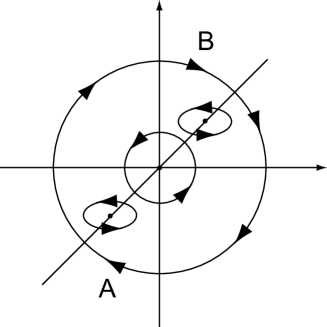
Figure 4: Contour, which is used to find the index of complex singular point.

$$\sum_{i}J_{i}+J(0)+J_{s}=0,$$ (81)

where $J_{s}-$ is the index of outside circle $S$, $\sum_{i}J_{i}-$ is the sum of indices of all internal simple singular points. This means, that the index of vortex structure, which is surrounded by contour $S$, is equal to:

$$J_{A}+J_{B}+J(0)=1.$$ (82)

Since index of hyperbolic points $A$ and $B$ is equal to $(-1)$, then the equation (82), gives index of complex singular point $J(0)=+3$.

2) Now, let us examine the case $n=3$ (dipole plus pole of order $n=3$). In this case the polynomial $P_{n-2}(z)$ is not trivial: $P_{1}(z)=1-\frac{z}{D}$.

Function $\left|u_{3}(z)\right|^{2}$ has the form :

$$\left|u_{3}(z)\right|^{2}=\frac{1}{\left|D\right|^{4}}\left|\frac{D}{z}\right|^{2}\exp\left(\frac{D\overline{z}+\overline{D}z}{\left|z\right|^{2}}\right)\left|1-\frac{z}{D}\right|^{2},$$ (83)

or in the real form:

$$\left|u_{3}(z)\right|^{2}=\frac{1}{(x^{2}+y^{2})(D_{1}^{2}+D_{2}^{2})}\exp\left(2\frac{D_{1}x+D_{2}y}{x^{2}+y^{2}}\right)\times$$ (84)

$$\times\left[1+\frac{(x^{2}+y^{2})}{(D_{1}^{2}+D_{2}^{2})}-2\frac{(D_{1}x+D_{2}y)}{(D_{1}^{2}+D_{2}^{2})}\right].$$

Correspondingly the  stream function $\Psi$ has the form:

$$\Psi=-\ln 8+3\ln(x^{2}+y^{2})-2\frac{D_{1}x+D_{2}y}{x^{2}+y^{2}}+$$ (85)

$$+2\ln[1+\left|u_{3}(z)\right|^{2}],$$

where $\left|u_{3}(z)\right|^{2}$ is given by the formula (84). Stream lines picture is presented on (Fig.5) with $D_{1}=D_{2}=1.$ One can see that, unlike previous case, the elliptical point appears in the solution. Previous internal hyperbolic point splits into two. Structure of central singular point does not change, its index is still equal to 3.

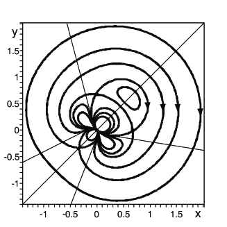
Figure 5: Vortex structure with n=3 (dipole and pole of order n=3). One can see, that the elliptic point appears. Internal singular hyperbolic point splits into two. Structure of central singular point does not change. Straight lines indicate, as earlier, exceptional directions of central singular point. Structure of the external separatrix does not change. Structure of internal separatrix which are now surrounding new elliptic points becomes more complex.

Note, that outside separatrix remains the same. It surrounds all  internal vortex structure, including new elliptical point around which appears the vortex with negative vorticity. The separatrix of previous hyperbolic internal point gets more complex because now it surrounds another additional elliptical point. All separatrix link hyperbolic points either with each other or with central singularity.

3) Now we consider the case $n=4$ (dipole plus pole of the order $n=4$). In this case the polynomial $P_{n-2}(z)$ has the form:

$$P_{2}(z)=1-2\left(\frac{z}{D}\right)+2\left(\frac{z}{D}\right)^{2}.$$ (86)

In the real form:

$$\left|P_{2}(z)\right|^{2}=1-4\frac{D_{1}x+D_{2}y}{(D_{1}^{2}+D_{2}^{2})}\left(1+2\frac{(x^{2}+y^{2})}{(D_{1}^{2}+D_{2}^{2})}\right)+$$ (87)

$$+4\frac{[(D_{1}^{2}-D_{2}^{2})(x^{2}-y^{2})+4D_{1}D_{2}xy]}{(D_{1}^{2}+D_{2}^{2})^{2}}+4\frac{(x^{2}+y^{2})}{(D_{1}^{2}+D_{2}^{2})}\left(1+\frac{(x^{2}+y^{2})}{(D_{1}^{2}+D_{2}^{2})}\right).$$

Function $\left|u_{4}(z)\right|^{2}$ takes the form:

$$\left|u_{4}(z)\right|^{2}=\frac{\left|P_{2}(z)\right|^{2}}{\left|D\right|^{2}\left|z\right|^{4}}\exp\left(\frac{D\overline{z}+\overline{D}z}{\left|z\right|^{2}}\right).$$ (88)

As a result for stream function we obtain the expression:

$$\Psi=-\ln 8+4\ln(x^{2}+y^{2})-2\frac{D_{1}x+D_{2}y}{x^{2}+y^{2}}+$$ (89)

$$+2\ln[1+\left|u_{4}(z)\right|^{2}].$$

The image of stream lines is presented on (Fig.6), with $D_{1}=D_{2}=1.$ (Butterfly). First of all one can see that two singular elliptical points appear and around them two satellites vortices. We can see also that there are four hyperbolic points. Separatrix structure becomes more complex. There are three groups of separatrix. First separatrix is of the same kind that outside separatrix in all previous cases. The second one is the same as the separatrix of internal hyperbolic point in first case. So a new group of separatrix appears which links vortices satellites (elliptical singular points) with the central singular point; the structure of the last one does not change from tropological point of view.

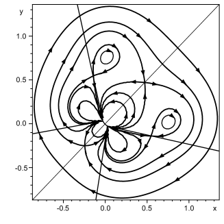
Figure 6: Vortex structure with n=4, ”butterfly”(dipole and pole of order n=4). One can see, that two elliptic singular points appear with two vortices satellites. Besides, one new group of separatrix appears, whiich connects vortices satellites with the central singular point.Topological structure of separatrix of external and internal hyperbolic points does not change.

4). Let us examine poles of higher order :$n=5$, i $n=6.$ Correspondingly polynomials $P_{n-2}(z)$ have the form:

$$P_{3}(z)=1-3\left(\frac{z}{D}\right)+6\left(\frac{z}{D}\right)^{2}-6\left(\frac{z}{D}\right)^{3},$$ (90)

$$P_{4}(z)=1-4\left(\frac{z}{D}\right)+12\left(\frac{z}{D}\right)^{2}-24\left(\frac{z}{D}\right)^{3}+24\left(\frac{z}{D}\right)^{4}.$$ (91)

Stream lines with $n=5$ are presented on (Fig.7), with $D_{1}=D_{2}=1.$ In this case three elliptical singular points appear (three vortices satellites) and five hyperbolic singular points. In case of $n=6$, four elliptical singular points appear and six hyperbolic singular points. With the increasing of number $n$ there are always $n$- hyperbolic singular points and $n-2$ elliptical points. Central singular point conserves four exceptional directions, i.e. its index remains equal to 3. Appeared vortex structure has symmetry relative to square diagonal. Diagonal pass always by central singular points and by opposite singular point, which is hyperbolic with $n=2k,$ and elliptical with $n=2k+1.$ The obtained vortex structure has the form of necklace composed of vortices satellites except the low sector, which always has hyperbolic singular point, linked by separatrix with central singularity.

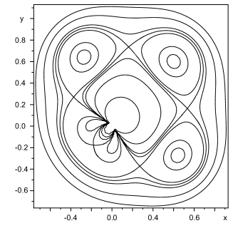
Figure 7: Vortex structure with n=5. In this case three elliptic singular points appear (three vortices satellites) and 5 hyperbolic points.

6 Discussions and conclusions

In this work we want to call attention to the fact that there are exact solutions of 2D-Euler equation which contain point singularities more complex, than singularities which are usually considered as typical ones for 2D-Euler equation. Such complex singularities can be non stationary [48], or stationary as well. Let us remind, that complex singularities are defined as singular points of vector field, which have the index $\left|J\right|\geq 2$ . The simplest singularity of this type is the dipole one with the index $J=2$. Point vortices and dipole singularities form a set of moving singularities in 2D-Euler equation, which dynamics is Hamiltonian [48]. With $f(\Psi)=0$, for general case, moving singularities can be only point vortices and  point dipoles. It means, that its index can not exceed two.  The reason for this, as it was shown earlier, that there are self-interaction of multipoles and overdetermination of their motion equations.

Now let us examine the case when in expansion (8) the function $f(\Psi)\neq 0.$ Consider more specifically the anzatz (8) in the form:

$$\Delta\Psi=f(\Psi)-\Gamma_{0}\delta(\overrightarrow{x}-\overrightarrow{x}_{0})-\overrightarrow{D}\frac{\partial}{\partial\overrightarrow{x}}\delta(\overrightarrow{x}-\overrightarrow{x}_{0}).$$ (92)

It is not difficult to see, that with $f(\Psi)=0$, there is no stationary solutions for 2D-Euler equation because $\left\{\Delta\Psi,\Psi\right\}\neq 0$. If the function $f(\Psi)\neq 0$ and is chosen in the Stuart’s form:

$$f(\Psi)=\exp(-\Psi),$$ (93)

the situation change substantially, what can be seen from results of this work. Presence of smooth part of vorticity field in the equation (92) gives exact solutions with the more complex singularity of index 3. As it is shown in this work, the singularity of vector field of index 3 can be interpreted in complex form as a fusion in function $u^{{}^{\prime}}(z)$ (60) of the pole, which corresponds to point vortex, with essential singular point which corresponds to point dipole. In real form, as it can be seen from the equation (75), for the final stream function the essential singularity splits up into singularities of point vortex and point dipoles types. However, the fusion of these singularities leads to a singular point with more complex geometry with a vector field index equal to three. This can be interpreted as the sum of the indexes of the point vortex and the point dipole.Exact localized solutions obtained in this work describe vortex structure of the complex form, where the singular point is surrounded be vortices satellites. With increasing of the number $n$  the vortices satellites have tendency to form symmetrical necklaces. The existence of  exact solutions with complex singularities itself is an important fact that is why in this work we contented ourself with consideration of simplest class of exact solutions expressed in elementary functions. We did not deal with questions of the construction of more complex solutions expressed by special functions and with important questions of stability of vortex configurations with complex singular points. All these questions must be examined separately and some of them will be studied in next works.

7 Appendix. Action of derivatives of $\delta-$function on velocity field

For convenience we present in this Appendix some formulae used in this work. It is well known (see, for example, [52] ), that generalized functions are linear functionals, which are acting in the space of basic functions $\{\varphi(x)\}.$ By definition, the  derivative $\delta^{{}^{\prime}}(x)$ acts on differentiable function $a(x)$ according to formula:

$$\int\delta^{{}^{\prime}}(x)a(x)\varphi(x)dx=-\int\delta(x)a^{{}^{\prime}}(0)\varphi(x)dx-\int\delta(x)a(0)\varphi^{{}^{\prime}}(x)dx=$$ (94)

$$=-\int\delta(x)a^{{}^{\prime}}(0)\varphi(x)dx+\int\delta^{{}^{\prime}}(x)a(0)\varphi(x)dx;\forall\varphi(x).$$

This gives a well known formula:

$$a(x)\delta^{{}^{\prime}}(x)=-a^{{}^{\prime}}(x)\delta(x)+a(0)\delta^{{}^{\prime}}(x)$$ (95)

Derivative of order $(k)$ acts on infinitely differentiable function $a(x)$, according to formula (96), which is obtained in a similar manner (94), as a result of integration by parts:

$$a(x)\delta^{(k)}(x)=\sum_{j=0}^{k}(-1)^{j+k}C_{k}^{j}a^{(k-j)}(0)\delta^{(j)}(x).$$ (96)

We need to use now particular cases: $k=2$:

$$a(x)\delta^{{}^{\prime\prime}}(x)=a^{{}^{\prime\prime}}(0)\delta(x)-2a^{{}^{\prime}}(0)\delta^{{}^{\prime}}(x)+a(0)\delta^{{}^{{}^{\prime\prime}}}(x),$$ (97)

and $k=3:$

$$a(x)\delta^{{}^{{}^{\prime\prime\prime}}}(x)=-a^{{}^{\prime\prime\prime}}(0)\delta(x)+3a^{{}^{\prime\prime}}(0)\delta^{{}^{\prime}}(x)-3a^{{}^{\prime}}(0)\delta^{{}^{\prime\prime}}(x)+a(0)\delta^{{}^{{}^{\prime\prime\prime}}}(x).$$ (98)

From formula (96) one can see that the derivative of order $(k)$ from $\delta-$ function engenders also all derivatives of lower orders including terms without derivatives, i.e.simply $\delta-$ functions. Similar formulae are obtained also for the case of multiple variables. In particular, for two variables $x_{i_{1}},x_{i_{2}}$ the second derivative acts according the formula:

$$a(\overrightarrow{x})\frac{\partial^{2}}{\partial x_{i_{1}}\partial x_{i_{2}}}\delta(\overrightarrow{x})=\left[\frac{\partial^{2}a(\overrightarrow{x})}{\partial x_{i_{1}}\partial x_{i_{2}}}\mid_{\overrightarrow{x}=0}\right]\delta(\overrightarrow{x})-\left[\frac{\partial a(\overrightarrow{x})}{\partial x_{i_{2}}}\mid_{\overrightarrow{x}=0}\right]\frac{\partial\delta(\overrightarrow{x})}{\partial x_{i_{1}}}-$$ (99)

$$-\left[\frac{\partial a(\overrightarrow{x})}{\partial x_{i_{1}}}\mid_{\overrightarrow{x}=0}\right]\frac{\partial\delta(\overrightarrow{x})}{\partial x_{i_{2}}}+a(0)\frac{\partial^{2}\delta(\overrightarrow{x})}{\partial x_{i_{1}}\partial x_{i_{2}}}$$

References

[1] H.Lamb, Hydrodynamics, 6th ed.Cambridge University
Press, Cambridg,1932.
[2] P.G.Saffman, Vortex Dynamics, Cambridge University
Press, Cambridge,1992.