Phase space structure and dynamics within the time-dependent Hartree-Fock approach
Abstract
We study the equilibration and relaxation processes within the time-dependent Hartree-Fock approach using the Wigner distribution function. On the technical side we present a geometrically unrestricted framework which allows us to calculate the full six-dimensional Wigner distribution function. With the removal of geometrical constraints, we are now able to extend our previous phase-space analysis of heavy-ion collisions in the reaction plane to unrestricted mean-field simulations of nuclear matter on a three-dimensional Cartesian lattice. From the physical point of view we provide a quantitative analysis on the stopping power in TDHF. This is linked to the effect of transparency. For the medium-heavy 40Ca+40Ca system we examine the impact of different parametrizations of the Skyrme force, energy-dependence, and the significance of extra time-odd terms in the Skyrme functional. For the first time, transparency in TDHF is observed for a heavy system, 24Mg+208Pb.
pacs:
21.60.-n,21.60.JzI Introduction
Time-dependent Hartree-Fock (TDHF) theory provides a fully self-consistent mean-field approach to nuclear dynamics. First employed in the late 1970’s Bonche ; Svenne ; Negele ; Davies the applicability of TDHF was constrained by the limited computational power. Therefore, early applications treated the problem in only one spatial dimension, utilizing a very simplified parametrization of the nuclear interaction. Due to the increase in computational power, state-of-the-art TDHF calculations are now feasible in three-dimensional coordinate space, without any symmetry restrictions and using the full Skyrme interaction Kim ; Simenel ; Nakatsukasa ; Umar05a ; Maruhn1 ; Guo08a .
In this work the Wigner distribution function Wigner is calculated as an analysis tool to probe the phase space behavior in TDHF evolution of nuclear dynamics. In comparison to previous work Loebl , where the Wigner analysis was performed in one and two dimensions, we are now able to carry out both the TDHF simulation and the phase-space analysis in three dimensions. Transformation from coordinate-space representation to phase-space representation, i.e. calculating the Wigner distribution from the density matrix, still remains a computationally challenging problem. Here, we present a fully three-dimensional analysis which allows the study of relaxation processes simultaneously in all directions in -space. An early one-dimensional study of the Wigner function for TDHF can be found in Maruhn3 .
The paper is outlined as follows: In Sec. II we introduce the Wigner distribution function and discuss the numerical framework used in this work. Some benchmark results are presented to give an idea about the computational resources necessary to compute the Wigner function. We then introduce the principal observables summarizing the local or global momentum-space properties of the Wigner function. First the quadrupole operator in momentum space which gives rise to the usual deformation parameters and to probe relaxation procecces in dynamical calculations. In addition, we define an estimate for the occupied phase-space volume to obtain a relation between the fragment separation in momentum and coordinate space.
Sec. III illustrates the geometrical structure of the Wigner distribution by means of momentum cuts for a few static nuclei. This is followed by a detailed discussion of the central 40Ca+40Ca collision, paying particular attention to the effect of transparency. We discuss the impact of different Skyrme parametrizations on the relaxation behavior, as well as the dependence on the center-of-mass energy for a fixed Skyrme interaction. We also examine the influence of extra time-odd terms in the Skyrme functional. We complete this issue by looking at the 24Mg+208Pb reaction, where transparency can be studied for the case of a heavy system.
II Outline of formalism
II.1 Solution of the TDHF equations
The TDHF equations are solved on a three-dimensional Cartesian lattice with a typical mesh spacing of fm. The initial setup of a dynamic calculation needs a static Hartree-Fock run, whereby the stationary ground states of the two fragments are computed with the damped-gradient iteration algorithm Blum ; Reinhard . The TDHF runs are initialized with energies above the Coulomb barrier at some large but finite separation. The two ions are boosted with velocities obtained by assuming that the two nuclei arrive at this initial separation on a Coulomb trajectory. The time propagation is managed by utilizing a Taylor-series expansion of the time-evolution operator Flocard up to sixth order with a time step of fm/c. The spatial derivatives are calculated using the fast Fourier transforms (FFT).
II.2 Computing the Wigner function
The Wigner distribution function is obtained by a partial Fourier transform of the density matrix , with respect to the relative coordinate
| (1) | |||||
| (2) |
Because is not positive definite, it is misleading to consider the Wigner function as a phase-space probability distribution. We will refer to the appearance of negative values for in Sec. III.
Evaluating the Wigner function in six-dimensional phase space is still a computational challenge and only possible employing full Open MP parallelization and extensive use of FFT’s. The determing factor is the grid size, which results in
| (3) |
steps to provide the Wigner transform in full space, where are the grid points in each direction.
Figure 1 shows the time taken to evaluate the Wigner function for one single time-step on a grid for a 16O+16O collision. Benchmarks are shown for two different CPU’s. Storing the Wigner function reduced to the reaction plane, i.e. at one time step will consume Mb of disk space for the presented case in Fig. 1. Going to larger grid sizes, needed for heavier systems, and/or storing the full three-dimensional Wigner function will clearly result in entering the Gb regime.
II.3 Observables
In this section we discuss some of the observables used in our analysis. In order to avoid any misunderstandings we will label all observables evaluated in momentum space with a subscript , and all observables in coordinate space with a subscript .
II.3.1 Quadrupole in momentum space
As an observable to probe relaxation in phase-space quantitatively, we evaluate the quadrupole operator in momentum space. The local deviation of the momentum distribution from a spherical shape is a direct measure for equilibration. The local quadrupole tensor in -space is given by
| (4) |
using the -th moment from the local momentum distribution
| (5) |
with denoting the average local flow
| (6) |
The spherical quadrupole moments and are computed by diagonalization of
| (7) | |||||
| (8) |
with labeling the eigenvalues of . Switching to polar notation the observables
| (9) | |||||
| (10) |
are obtained via the dimensionless quantities
| (11) | |||||
| (12) |
where
| (13) |
accounts for the local rms-radius in -space. The norm is defined such that
| (14) |
In the presented formalism it is straightforward to define global observables. The global quadrupole tensor is calculated by spatial integration
| (15) |
Applying the same diagonalization as in the local case (7) we end up with a global definition for and . For the following results we will mainly use the global definition since it is more compact and allows the simultaneous visualization of multiple time-dependent observables. We will however show some local results in Sec. III.3.
II.3.2 Quadrupole in coordinate space
To illustrate the global development of a reaction, we will also use the expectation value of the quadrupole operator in coordinate space.
II.3.3 Occupied phase space volume
To give a rough measure for the phase-space volume occupied by the fragments during a heavy-ion collision we assume a spherical shape of the local momentum distribution. Adding up the -spheres
| (16) |
leads to the total occupied phase-space volume
| (17) |
III Results and discussion
It is the aim of this work to provide a quantitative analysis of the magnitude of relaxation processes occurring in TDHF. Therefore we will vary a single reaction parameter, while all the other parameters are fixed. The 40Ca+40Ca-system provides a suitable test case. The occurrence of transparency will also be examined for the heavy 24Mg+208Pb system. However, we first start with a brief discussion concerning the geometrical structure of the full Wigner distribution for static nuclei.
III.1 Static nuclei
In this section we present slices through the full six-dimensional Wigner distribution for some static nuclei. For this purpose the Wigner distribution is plotted at the spatial center, and for fixed momentum in the -direction, i.e. .
Starting with 16O, which corresponds to subplot (a) in Fig. 2, the Wigner function reveals strong negative values at the center. The hole in the momentum distribution, which indicates the influence of distinct shell effects, was already visible in the lower-dimensional analysis Loebl , however in that case it corresponded to small positive values.
Considering heavier nuclei, we observe the appearance of two holes for case (b), reflecting the deformation of 24Mg in coordinate space. In contrast we find a pronounced peak for 40Ca, case (c). The momentum distribution for 208Pb in subplot (d) reveals again a central hole which this time is positive. This agrees with the reduction in the spatial density observed for 208Pb.
Although the geometrical structure differs from nucleus to nucleus, it is important to note that for cold ground-state nuclei the momentum distribution differs considerably from a Fermi distribution, even for a heavy nucleus.
III.2 40Ca+40Ca
We now investigate the relaxation process in momentum space for heavy-ion reactions. We have chosen the 40Ca+40Ca-system as a benchmark to investigate the quantitative effect of some parameters on the relaxation process. All calculations in this section were done for central collisions (impact parameter ). The numerical grid was set up with grid points.
III.2.1 Variation of the Skyrme force
In the first set of calculations we vary the Skyrme parametrization. Figure 3 shows the results of a central 40Ca+40Ca collision with the Skyrme parametrizations SLy4, SLy6 Chabanat , SkMs Bartel , SkI3, and SkI4 Reinhard2 . While SkMs was chosen as an example for an outdated interaction, the SLy(X) set of forces was originally developed to study isotopic trends in neutron rich nuclei and neutron matter with applications in astrophysics. The SkI(X) forces take the freedom of an isovector spin-orbit force into account. This results in an improved description of isotopic shifts of r.m.s. radii in neutron-rich Pb isotopes.
The global development of the reaction is visualized in subplot (d). The time-dependent expectation value shows the five trajectories initially in good agreement but finally fanning out. A similar splitting behavior depending on the employed Skyrme parametrization was already found in Maruhn85 . While the two Sk(X)-forces show a full separation of the two fragments, there is a slight remaining contact between the fragments for the case of SLy6, which will result in complete separation in a longer calculation. However the trajectories for SLy4 and SkMs show a merged system in the final state, which was found to persist in long-time simulations.
We now consider the relationship between the observed characteristics in coordinate space with the dynamics in phase space. Subplot (a) shows the -value, measuring the global deviation of the momentum distribution from a sphere. The initial -peak is strongly damped for all five Skyrme-forces. While the time development for all parametrizations remain in phase up to the second peak, later it starts to vary and continue with damped oscillations. For a better visualization the first peak is magnified in subplot (e). The taller the -peak the longer the fragments will stick together in coordinate space. The effect appears to depend on the effective mass . Smaller effective masses give rise to a smaller -deformation. Table 1 summarizes the -values associated with the maximal deformations for all the Skyrme forces used in this work.
| Skyrme force | ||
|---|---|---|
| SkM∗ | 0.79 | 0.0116 |
| SLy4 | 0.70 | 0.0111 |
| SLy6 | 0.69 | 0.0106 |
| SkI4 | 0.65 | 0.0102 |
| SkI3 | 0.57 | 0.0095 |
Subplot (b) shows the -value which indicates, whether a deformation is prolate, oblate, or triaxial Greiner . For the present scenario of a central collision the -value jumps between prolate and oblate configurations indicating that the momentum distribution oscillates between being aligned primarily in the beam direction or transverse to it. For the sake of completeness we additionally present the occupied phase-space volume (c) which will prove more useful for the next reaction parameter to be discussed: the center-of-mass energy.
III.2.2 Variation with the center-of-mass energy
As a second reaction parameter the center-of-mass energy, , is varied. Results are presented for energies ranging from MeV/nucleon up to MeV/nucleon. The Skyrme interaction now is fixed to be SkI4. For the case of the lowest (highest) energy Video III.2.2 (Video III.2.2) provides a video visualizing the reaction in phase space. The calculation done with the lowest energy MeV shows two fully separated fragments in the exit channel. In contrast, the case with the highest energy (as well as the one at an intermediate energy) results in a merged system. The global observables are plotted in Fig. 4. It may not be obvious at first why the fragments should split for lower energies and merge for higher ones. But the estimate for the occupied phase-space volume presented in subplot (c) indicates that increases with energy. Therefore the fragments’ average distance in phase space is larger, while in compensation they can come closer to each other in coordinate space. However, this behavior is also dependent on the particular Skyrme force used and the presence of time-odd terms, which is discussed in the next subsection.
![[Uncaptioned image]](/html/1201.5269/assets/x10.png) \setfloatlink
\setfloatlink
http://th.physik.uni-frankfurt.de/ loebl/vid1.mpeg
(color online)
Two-dimensional --slice from the full six-dimensional Wigner distribution
for a central 40Ca+40Ca collision
with a center-of-mass energy of MeV.
{video}
![[Uncaptioned image]](/html/1201.5269/assets/x11.png) \setfloatlinkhttp://th.physik.uni-frankfurt.de/ loebl/vid2.mpeg
(color online)
Same as Video III.2.2 with a center-of-mass energy of
MeV.
\setfloatlinkhttp://th.physik.uni-frankfurt.de/ loebl/vid2.mpeg
(color online)
Same as Video III.2.2 with a center-of-mass energy of
MeV.
III.2.3 Influence of time-odd terms
Skyrme energy-density functionals are calibrated to ground state properties of even-even nuclei Chabanat ; Bartel ; Reinhard2 . This leaves the choice of the time-odd terms in the functional (current , spin-density , spin kinetic energy density , and the spin-current pseudotensor ) largely unspecified BH03 . Galilean invariance requires at least some of these terms to be present depending on the presence of the associated time-even term, e.g. for the combination. In our calculations we always include the time-odd part of the spin-orbit interaction. In order to investigate the effects of the remaining time-odd terms, we have compared different choices by using a single Skyrme parametrization and the same test case. We choose the force SLy4 and start with the minimum number of time-odd terms which is needed to ensure Galilean invariance Eng75a . In the next stage, we include also the spin-density terms proportional to . Finally, we also add the combination which includes the tensor spin-current term . As shown in Fig. 5, at least for the quantities and , varying these time-odd terms has a very little effect in the initial contact phase and the dynamical behavior becomes somewhat different only in later stages of the collision. On the other hand, small differences near the threshold energy (the highest collision energy for a head-on collision that results in a composite system. At higher energies the nuclei go through each other) can have large long-term effects on the outcome of the collision. For example a small difference in dissipation may be enough to influence the decision between re-seperation or forming a composite system. We have also checked a broader range of collision energies from the fusion regime up to deep inelastic collisions. The interesting quantity is the loss of fragment kinetic energy between the entrance and exit channels. It was found that the spin terms contribute small changes to this loss which can go in both directions, less dissipation near fusion threshold and more dissipation above. Subplot (b) of Fig. 5 shows the effects near the Coulomb barrier where spin terms reduce dissipation.
III.3 24Mg+208Pb
The study of the 24Mg+208Pb reaction is motivated by experiments indicating some evaporation of heavy nucleon clusters around zero degree relative to the beam direction in the 25Mg+206Pb collision Heinz . The following results are obtained on a grid with Skyrme interaction SLy6.
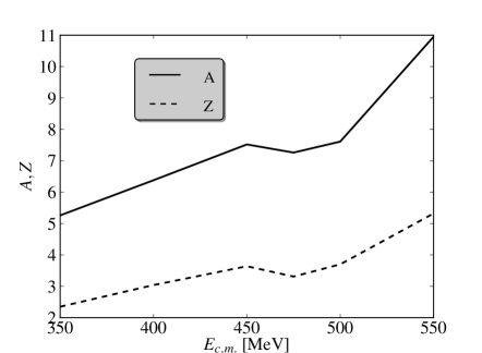
In the following we define as ”feed-through” the mass and charge numbers of the nuclear matter cluster emitted in the forward direction. Fig. 6 shows TDHF results on the feed-through for central 24Mg+208Pb reactions. However, the density of the emerging fragments is very low. We identify the energy threshold for a possible feed-through at MeV.
![[Uncaptioned image]](/html/1201.5269/assets/x19.png) \setfloatlink
\setfloatlink
http://th.physik.uni-frankfurt.de/ loebl/vid3.mpeg (color online) Two-dimensional --slice from the full six-dimensional Wigner distribution for a central 24Mg+208Pb collision with a center-of-mass energy of MeV.
Video III.3 provides a video showing the central 24Mg+208Pb reaction slightly above the feed-through threshold in the Wigner picture. As time elapses 24Mg is absorbed into the phase-space volume of 208Pb. We observe a rotation of phase-space density inside the merged system. After a short time a jet is visible, leaving the 24Mg+208Pb compound. This corresponds to low-density fragment in coordinate space with a total mass comparable to an particle for the actual energy.
In Fig. 7 we compare the global observables for a central and a peripheral reaction with impact parameter fm. Subplot (a) shows that the -peaks are diminished for the case of the non-central collision. In this case we find that the alignment of the momentum distribution probed via the -angle (b) no longer shows a sharp transition between a prolate and an oblate configuration. The smoother development of is due to the possibility for triaxial configurations in the non-central collision.
![[Uncaptioned image]](/html/1201.5269/assets/x23.png) \setfloatlink
\setfloatlink
http://th.physik.uni-frankfurt.de/ loebl/vid4.mpeg (color online) The local observable is plotted in the reaction plane, i.e. for a 24Mg+208Pb collision. The calculation is done with Skyrme force SLy6 and a center-of-mass energy of MeV.
The time development of the local observable can be studied in Video III.3. At fm/c we observe a non vanishing local deformation in the 24Mg fragment. As we have previously shown in Fig. 2 (b), 24Mg reveals a ground state deformation in coordinate as well as in momentum-space. In the reaction plane a domain of high values occurs while 24Mg is penetrating through the 208Pb fragment. The initial disturbance travels through the lead fragment while it exhibits a strong decrease in magnitude. When the low density nuclear cluster leaves the merged system, the excitation has completely subsided.
IV Summary
We have presented a geometrically unrestricted framework to study nuclear dynamics within TDHF in the full six-dimensional phase space. The impact of different reaction parameters on the outcome of a heavy-ion collision was studied in detail for 40Ca+40Ca and 24Mg+208Pb systems. We find that there is transparency in both collisions, which is clearly reflected in the global asymmetry of the Wigner momentum distribution. The surprising result that in some cases the system merges at higher energies and shows transparency at lower ones can be related to the interplay between momentum- and configuration-space volumes which is a reflection of the Pauli principle. It is also interesting that the two distributions in phase-space never truly combine to form a single distribution. This clearly indicates that two-body collisions will be necessary to achieve true equilibrium as the reaction proceeds to longer contact times. The detailed degree of relaxation found depends on energy and also the properties of the Skyrme force, where especially the effective mass seems to be important. The presence of additional time-odd terms in the Skyrme functional appears to have a complex impact on the outcome of a collision as well. In this paper only one non-central collision was studied. A systematic investigation of impact parameter and energy dependence as well as even heavier systems would be highly interesting but is beyond computational feasibility at the moment.
Acknowledgment
This work has been supported by by BMBF under contract Nos. 06FY9086 and 06ER142D, and the U.S. Department of Energy under grant No. DE-FG02-96ER40963 with Vanderbilt University. The videos linked in the manusscript can be found at http://th.physik.uni-frankfurt.de/~loebl/vid1.mpeg, http://th.physik.uni-frankfurt.de/~loebl/vid2.mpeg, http://th.physik.uni-frankfurt.de/~loebl/vid3.mpeg, and http://th.physik.uni-frankfurt.de/~loebl/vid4.mpeg.
Appendix A The full Skyrme functional
Following the convention used in Ref. Les07 we can write down the full Skyrme energy density functional . It depends on seven local densities and currents, namely the spatial density (time-even), the kinetic density (time-even), the current density (time-odd), the spin density (time-odd), the spin-current density (time-even), and the tensor kinetic density (time-odd). They are defined as
| (18) | |||||
with
| (19) |
We will consider the recoupled forms of the proton and neutron densities to isoscalar and isovector densities. The recoupling of the density , for example, yields
| (20) |
The Skyrme full functional now reads
| (21) | |||||
The functional accounts for the central, tensor, and spin-orbit interaction. All possible bilinear terms up to second order in the derivatives are included. The coupling constants of the central and tensor part are listed below in terms of the well known Skyrme parameters
| (22) |
The coupling constants of the spin-orbit part of the functional can be rewritten into the form
| (23) |
References
- (1) P. Bonche, S. E. Koonin, and J. W. Negele, Phys. Rev. C 13, 1226 (1976).
- (2) J. P. Svenne, Adv. Nucl. Phys. 11, 179 (1979).
- (3) J. W. Negele, Rev. Mod. Phys. 54, 913 (1982).
- (4) K. T. R. Davies, K. R. S. Devi, S. E. Koonin, and M. R. Strayer, in Treatise on Heavy-Ion Physics, Vol. 3 Compound System Phenomena, edited by D. A. Bromley (Plenum Press, New York, 1985), p. 3.
- (5) K.-H. Kim, T. Otsuka, and P. Bonche, J. Phys. G 23, 1267 (1997).
- (6) C. Simenel and P. Chomaz, Phys. Rev. C 68, 024302 (2003).
- (7) T. Nakatsukasa and K. Yabana, Phys. Rev. C 71, 024301 (2005).
- (8) A. S. Umar and V. E. Oberacker, Phys. Rev. C 71, 034314 (2005).
- (9) J. A. Maruhn, P.-G. Reinhard, P. D. Stevenson, J. R. Stone, and M. R. Strayer, Phys. Rev. C 71, 064328 (2005).
- (10) Lu Guo, P.–G. Reinhard, and J. A. Maruhn, Phys. Rev. C, 77, 041301 (2008).
- (11) E. P. Wigner, Phys. Rev 40, 749 (1932).
- (12) N. Loebl, J. A. Maruhn, and P.-G. Reinhard, Phys. Rev. C 84, (2011).
- (13) J. A. Maruhn, Proc. Topical Conf. on Heavy-ion collisions, Oak Ridge National Laboratory report CONF-770602, Fall Creek Falls State Park, TN (1977).
- (14) V. Blum, G. Lauritsch, J. A. Maruhn, and P.-G. Reinhard, J. Comput. Phys. 100, 364 (1992).
- (15) P.-G. Reinhard and R. Y. Cusson, Nucl. Phys. A378, 418 (1982).
- (16) H. Flocard, S. E. Koonin, and M. S. Weiss, Phys. Rev. C17 (1978) 1682-1699.
- (17) E. Chabanat, E. P. Bonche, P. Haensel, J. Meyer, and R. Schaeffer, Nucl. Phys. A 635, 231 (1998).
- (18) J. Bartel, P. Quentin, M. Brack, C. Guet, and H.-B. Hkansson, Nucl. Phys. A386, 79 (1982).
- (19) P.-G. Reinhard and H. Flocard, Nucl. Phys. A 584, 467 (1995).
- (20) J. A. Maruhn, K. T. R. Davies, M. R. Strayer, Phys. Rev. C31, 1289-1296 (1985).
- (21) W. Greiner, and J.A. Maruhn, “Nuclear models”, Springer-Verlag, Berlin, New York (1996).
- (22) S. Heinz, V. Comas, F. P. Heßberger, S. Hofmann, D. Ackermann, H. G. Burkhard, Z. Gan, J. Heredia, J. Khuyagbaatar and B. Kindler, et al., The European Physical Journal A - Hadrons and Nuclei, Springer Berlin / Heidelberg, 2008, 38, 227-232.
- (23) M. Bender, P.-H. Heenen, and P.-G. Reinhard, Rev. Mod. Phys. 75, 121 (2003).
- (24) Y. M. Engel, D. M. Brink, K. Goeke, S. J. Krieger, and D. Vautherin, Nucl. Phys. A 249, 215 (1975).
- (25) T. Lesinski, M. Bender, K. Bennaceur, T. Duguet, and J. Meyer, Phys. Rev. C76, 014312 (2007).