Zitterbewegung of electrons in quantum wells and dots in presence of an in-plane magnetic field

Abstract

We study the effect of an in-plane magnetic field on the $zitterbewegung$ (ZB) of electrons in a semiconductor quantum well (QW) and in a quantum dot (QD) with the Rashba and Dresselhaus spin-orbit interactions. We obtain a general expression of the time-evolution of the position vector and current of the electron in a semiconductor quantum well. The amplitude of the oscillatory motion is directly related to the Berry connection in momentum space. We find that in presence of the magnetic field the ZB in a quantum well does not vanish when the strengths of the Rashba and Dresselhaus spin-orbit interactions are equal. The in-plane magnetic field helps to sustain the ZB in quantum wells even at low value of $k_{0}d$ (where $d$ is the width of the Gaussian wavepacket and $k_{0}$ is the initial wave vector). The trembling motion of an electron in a semiconductor quantum well with high Lande g-factor (e.g. InSb) sustains over a long time, even at low value of $k_{0}d$. Further, we study the ZB of an electron in quantum dots within the two sub-band model numerically. The trembling motion persists in time even when the magnetic field is absent as well as when the strengths of the SOI are equal. The ZB in quantum dots is due to the superposition of oscillatory motions corresponding to all possible differences of the energy eigenvalues of the system. This is an another example of multi-frequency ZB phenomenon.

I Introduction

In recent years there is a growing interest in the field of spin based electronic devices. There has been a lot of study in this field after the proposal of the spin field effect transistor by Datta and Das datta . The charge carriers carry spin in addition to their charges. The ultimate goal of this field is to control the spin degree of freedom of the charge carriers to produce and detect spin-polarized current in semiconductor nanostructures fabian . One can develop device technology wolf and quantum information processing david in future on the basis of the manipulation of the spin degree of freedom. The coupling between intrinsic spin of an electron with its orbital angular momentum constitutes the intrinsic spin-orbit interaction (SOI) in low-dimensional semiconducting systems. Particularly, there are two kind of SOI present in low-dimensional semiconductor structures. One is the Rashba rashba spin-orbit interaction (RSOI) and another is the Dresselhaus dress spin-orbit interaction (DSOI). The RSOI arises mainly from the inversion asymmetry of the confining potential in semiconductor heterojunctions. The strength of RSOI is proportional to the electric field externally applied which can be tuned by an external bias nitta ; mats or internally generated due to the crystal potentials. On the other hand DSOI is present in bulk materials and semiconductor heterostructures which lack bulk inversion symmetry. The form of DSOI term strongly depends on the growth direction of semiconductor quantum well (QW) car ; chen ; andr . The strength of DSOI depends on properties of the material and the crystal structure.

In 1930, Erwin Schrodinger Schro predicted that a free particle described by the relativistic Dirac equation will perform an oscillatory motion which is known as the $zitterbewegung$ (ZB). The free relativistic Dirac particle has two energy branches: $\epsilon({\bf p})=\pm\sqrt{{{{m}_{0}}^{2}}c^{4}+{c^{2}}{p^{2}}}$. It is well understood that this oscillatory motion results from the interference between these two energy branches huang . The large oscillation frequency $\omega_{{}_{c}}\simeq 10^{21}$ Hz and the small oscillation amplitude $\lambda_{c}\simeq 10^{-13}$ m is not accessible to the modern experimental techniques. Most of the studies on the ZB of electrons used plane waves to describe the electrons. It was pointed out by Lock lock that plane wave is not a localized state and therefore, rapid oscillations on the average position of a plane wave has some limitations. He also demonstrated that when an electron is described by a wave packet, the ZB oscillation has a transient character.

In 2005, Zawadzki et al. zawadki studied ZB in narrow gap semiconductor (NGS) by using the analogy between $\bf k\cdot\bf p$ theory of the energy bands in NGS and the free Dirac relativistic equation for electrons. They found much more favorable amplitude and frequency of the oscillation than those in a vacuum for a free electron. At the same time, Schliemann et al. john ; loss has studied the ZB of an electron in III-V zincblende semiconductor QWs in the presence of the SOI thoroughly. The above studies initiated intense theoretical research on the ZB of electrons in various condensed matter systems review ; demi ; rusin ; rusin1 ; maksinova ; winkler ; lamata ; nature .

The proposal of an experimental scheme for observing ZB in ultra-cold clark atomic gases is also given. The trembling motion was proposed for photons in a two-dimensional photonic crystal and for Ramsey interferometry photonic . It was reported in Ref. sonic that an acoustic analog of ZB in a macroscopic two-dimensional sonic crystal was observed. A general theory of ZB of a multi-band Hamiltonian is studied by David and Cserti cserti . Recently, Vaseghi vaseghi et al. studied the effect of an external perpendicular magnetic field on the ZB for both quantum wire and quantum dot within the two-sub-band model.

The dimensionless parameter $p_{0}=k_{0}d$ dictates whether the motion will be oscillatory or not. It was shown in Ref. [14] that the motion will be oscillatory when $p_{0}\gg 1$. It was also shown that the ZB vanishes when the strengths of the RSOI and DSOI are equal. This is due to an additional conserved quantity.

In this work we study effect of the in-plane magnetic field on the ZB of electrons in a semiconductor QW and in a QD with the Rashba and Dresselhaus SOI. We obtain an analytical expression of the time-evolution of the position vector of an electron in a QW by using the Schrodinger picture. The advantage of using the Schordinger picture is to see the direct relation between the amplitude of the oscillatory motion and the Berry connection in momentum space. We find that in presence of the magnetic field the ZB in a quantum well does not vanish even when the strengths of the Rashba and Dresselhaus spin-orbit interactions are equal. The ZB in a QW sustains even at very low value of $k_{0}d$ due to the presence of the magnetic field. The trembling motion of an electron in a semiconductor QW with high Lande g-factor (e.g. InSb) sustains over a long time, even at very low value of $k_{0}d$. The time-period of the oscillation decreases as the magnetic field strength is increased. Next, we study the ZB of an electron in a QD within the two sub-band model numerically. The trembling motion does not fade away in time even when the magnetic field is absent as well as when the strength of the SOIs is equal.

This paper is organized as follows. In section II, we review the Hamiltonian and eigenstates of a 2DEG with both type of SOI in the presence of an in-plane magnetic field. In section III, we derive time-evolution of the electron’ position vector in the Schordinger picture. The numerical results and discussions are given in section V. Section VI contains the calculation and result of ZB of electrons in a GaAs/AlGaAs QD. The conclusion is presented in Section VII.

II Two-dimensional electron gas with spin-orbit interactions

We consider a 2DEG with the Rashba and Dresselhaus spin-orbit interactions in presence of an in-plane magnetic field ${\bf{B}}=\hat{x}{B}_{x}+\hat{y}{B}_{y}$. The single-particle Hamiltonian of this system is given by

$$H = \frac{{\bf p}^{2}}{2m^{\ast}}+\frac{\alpha}{\hbar}\big{(}{\sigma}_{x}{p}_{y}-{\sigma}_{y}{p}_{x}\big{)}+\frac{\beta}{\hbar}\big{(}{\sigma}_{x}{p}_{x}-{\sigma}_{y}{p}_{y}\big{)}$$ (1)

$$+ \frac{g^{\ast}}{2}{\mu_{{}_{B}}}\big{(}B_{x}\sigma_{x}+B_{y}\sigma_{y}\big{)},$$

where ${\bf p}$ and $m^{\ast}$ is the momentum and the effective mass of an electron, respectively. Here $\alpha$ and $\beta$ are the strengths of the Rashba and Dresselhaus spin-orbit interaction. The last term in the Hamiltonian is the Zeeman term due to the application of the in-plane magnetic field $\bf B$, $g^{\ast}$ is the effective Lande-g factor and $\mu_{{}_{B}}$ is the Bohr magneton. The energy eigenvalues and the corresponding eigenstates of the system chang ; rod are, respectively, given by

$$E_{\pm}({\bf k})=\frac{\hbar^{2}\big{(}k_{x}^{2}+k_{y}^{2}\big{)}}{2m^{\ast}}\pm\sqrt{C^{2}+D^{2}},$$ (2)

where $C=\alpha k_{y}+\beta k_{x}+g^{\ast}\mu_{{}_{B}}B_{x}/2$, $D=\alpha k_{x}+\beta k_{y}-g^{\ast}\mu_{{}_{B}}B_{y}/2$, and the spin eigenstates are

$$|k,+\rangle=\frac{1}{\sqrt{2}}\begin{pmatrix}1\\ -ie^{-i\theta_{k}}\end{pmatrix},\hskip 7.22743pt|k,-\rangle=\frac{1}{\sqrt{2}}\begin{pmatrix}-ie^{-i\theta_{k}}\\ 1\end{pmatrix},$$ (3)

with $\theta_{k}=\tan^{-1}(C/D)$.

In absence of the magnetic field, a new conserved quantity $\Sigma=\sigma_{x}-\sigma_{y}$ exists for $\alpha=\beta$ john_prl ; john_prb . In this situation, the spin eigenstates $|k,\pm\rangle$ become independent of the wave vector $k$ and therefore the ZB does not exist due to the absence of spin randomization john ; loss . The situation is completely different when the in-plane magnetic field is present. It is clear from Eq. (3) that the spin states are always function of $k$ even at $\alpha=\beta$ as long as ${\bf B}\neq 0$. Therefore, spin randomization occurs and we would expect to see the ZB which is shown in the next section.

II.1 Time-evolution of the wave packet and the Zitterbewegung

We shall use the Schordinger picture to analyze the time-evolution of the electron position vector. We represent the initial wave function of an electron by a Gaussian wave packet with initial spin polarization along the $z$ axis as given by

$$\psi\big{(}{\bf r},0\big{)}=\frac{1}{2\pi}\int\,d^{2}ka({\bf k},0)e^{i\bf k\cdot r}\left(\begin{array}[]{c}1\\ 0\end{array}\right),$$ (6)

where $a({\bf k},0)=d/(\sqrt{\pi})e^{-\frac{1}{2}d^{2}\big{(}{\bf k-k}_{0}\big{)}^{2}}$. Here, $d$ and ${\bf k}_{0}$ is the initial width and the initial wave vector of the wave packet, respectively. The time-evolution of the initial wave packet in the Schordinger representation can be obtained in the usual manner as $\psi({\bf r},t)=U(t)\psi({\bf r},0)$, where $U(t)=e^{-iHt/\hbar}$ is the time-evolution operator. After doing some straightforward algebra we obtain,

$$\psi({\bf r},t) = \frac{1}{2\pi}\int\ d^{2}ka({\bf k},0)e^{i\bf k\cdot r}e^{-i\frac{\hbar k^{2}}{2m^{\ast}}t}$$ (11)

$$\times \Big{\{}\cos[\omega({\bf k})t]\left(\begin{array}[]{c}1\\ 0\end{array}\right)-e^{i\theta_{k}}\sin[\omega({\bf k})t]\left(\begin{array}[]{c}0\\ 1\end{array}\right)\Big{\}},$$

where $\omega({\bf k})=\big{[}E_{+}({\bf k})-E_{-}({\bf k})\big{]}/(2\hbar)$.

Equation (11) is nothing but the Fourier transformation of the following function:

$$\phi({\bf k},t)=a({\bf k},0)e^{-i\frac{\hbar k^{2}}{2m^{\ast}}t}\left(\begin{array}[]{c}\cos[\omega({\bf k})t]\\ -e^{i\theta_{k}}\sin[\omega({\bf k})t]\end{array}\right).$$

The expectation value of position operator is then simply given by

$$\langle{\bf r}(t)\rangle=i\int d^{2}k\phi^{\dagger}({\bf k},t){\bf\nabla}_{\bf k}\phi({\bf k},t).$$ (13)

Now it is straightforward to show that

$$\langle{\bf r}(t)\rangle=\langle{\bf r}(0)\rangle + \frac{\hbar{\bf k}(0)}{m^{\ast}}t-\frac{1}{2}\int d^{2}k\left|a({\bf k,0})\right|^{2}\Big{(}{\bf\nabla}_{\bf k}\theta_{k}\Big{)}$$ (14)

$$\times \Big{\{}1-\cos[\omega({\bf k})t]\Big{\}}.$$

The last oscillatory term $\cos[\omega({\bf k})t]$ in Eq. (14) indicates the ZB. Two important observations can be made by analyzing Eq. (14). First, the amplitude of the ZB is directly proportional to the Berry connection $\langle k,\pm|i\frac{\partial}{\partial{\bf k}}|k,\pm\rangle={\bf\nabla}_{\bf k}\theta_{k}$. Second, for $\alpha=\beta$ the amplitude (or the Berry connection) of the oscillation does not vanish when the in-plane magnetic field is present. But it vanishes if the magnetic field is absent.

After substituting the expressions for $a({\bf k},0)$, ${\bf\nabla}_{\bf k}\theta_{k}$ in Eq. (14) and considering the initial velocity of the wave packet is along $y$-direction (i.e. $k_{0x}=0,k_{0y}=k_{0}$) one can easily obtain the following expressions

$$\langle x(t)\rangle = \frac{d}{2\pi}e^{-d^{2}k_{0}^{2}}\int^{2\pi}_{0}d\phi\int_{0}^{\infty}dqe^{-q^{2}+2dqk_{0y}\sin\phi}$$ (15)

$$\times \frac{q^{2}(1-\eta^{2})\sin\phi+q(\varepsilon_{x}+\eta\varepsilon_{y})}{Q^{2}}$$

$$\times \Big{[}1-\cos\Big{(}\frac{2\alpha}{\hbar d}tQ\Big{)}\Big{]},$$

and

$$\langle y(t)\rangle = \frac{\hbar k_{0y}}{m^{\ast}}t$$ (16)

$$+ \frac{d}{2\pi}e^{-d^{2}k_{0}^{2}}\int^{2\pi}_{0}d\phi\int_{0}^{\infty}dqe^{-q^{2}+2dqk_{0y}\sin\phi}$$

$$\times \frac{q^{2}(\eta^{2}-1)\cos\phi+q(\eta\varepsilon_{x}+\varepsilon_{y})}{Q^{2}}$$

$$\times \Big{[}1-\cos\Big{(}\frac{2\alpha}{\hbar d}tQ\Big{)}\Big{]},$$

where $Q^{2}=(q\cos\phi+\eta q\sin\phi-\varepsilon_{y})^{2}+(q\sin\phi+\eta q\cos\phi+\varepsilon_{x})^{2}$, $\eta=\beta/\alpha$, $q=kd$, $\varepsilon_{x}=g^{\ast}\mu_{{}_{B}}B_{x}d/(2\alpha)$ and $\varepsilon_{y}=g^{\ast}\mu_{{}_{B}}B_{y}d/(2\alpha)$.

From Eqs. (15) and (16) one can infer that ZB is absent in the limit $d\rightarrow 0$. On the other hand, as $d\rightarrow\infty$ the Gaussian approaches to a delta function i.e. $a({\bf k},0)=\delta({\bf k}-{\bf k}_{0})$ and in this limit we find an analytic expression for the ZB as given by

$$\langle x(t)\rangle = \frac{1}{2}\frac{(1-\eta^{2})k_{0y}+\frac{g^{\ast}\mu_{{}_{B}}}{2\alpha}(B_{x}+\eta B_{y})}{(k_{0y}+\frac{g^{\ast}\mu_{{}_{B}}B_{x}}{2\alpha})^{2}+(\eta k_{0y}-\frac{g^{\ast}\mu_{{}_{B}}B_{y}}{2\alpha})^{2}}$$ (17)

$$\times \Big{\{}1-\cos[\omega(k_{0y})t]\Big{\}},$$

and

$$\langle y(t)\rangle = \frac{\hbar k_{0y}}{m^{\ast}}t$$ (18)

$$+ \frac{1}{2}\frac{\frac{g^{\ast}\mu_{{}_{B}}}{2\alpha}(\eta B_{x}+B_{y})}{(k_{0y}+\frac{g^{\ast}\mu_{{}_{B}}B_{x}}{2\alpha})^{2}+(\eta k_{0y}-\frac{g^{\ast}\mu_{{}_{B}}B_{y}}{2\alpha})^{2}}$$

$$\times \Big{\{}1-\cos[\omega(k_{0y})t]\Big{\}}.$$

We also calculate the expectation values of the velocity of electron in $x$ and $y$ direction. They are given by

$$\langle v_{x}(t)\rangle = \frac{\partial\langle x\rangle}{\partial t}$$

$$= \frac{v_{{}_{R}}}{2\pi}e^{-d^{2}k_{0y}^{2}}\int^{2\pi}_{0}d\phi\int_{0}^{\infty}dqe^{-q^{2}+2dqk_{0y}\sin\phi}$$

$$\times \frac{q^{2}(1-\eta^{2})\sin\phi+q(\varepsilon_{x}+\eta\varepsilon_{y})}{Q}\sin\Big{(}\frac{2\alpha Q}{\hbar d}t\Big{)},$$

and

$$\langle v_{y}(t)\rangle = \frac{\hbar k_{0y}}{m^{\ast}}$$

$$+ \frac{v_{{}_{R}}}{2\pi}e^{-d^{2}k_{0y}^{2}}\int^{2\pi}_{0}d\phi\int_{0}^{\infty}dqe^{-q^{2}+2dqk_{0y}\sin\phi}$$

$$\times \frac{q^{2}(\eta^{2}-1)\cos\phi+q(\eta\varepsilon_{x}+\varepsilon_{y})}{Q}\sin\Big{(}\frac{2\alpha Q}{\hbar d}t\Big{)}.$$

Here, $v_{{}_{R}}=\Omega d=2\alpha/\hbar$ is the velocity corresponding to the RSOI. The corresponding currents are simply given by $\langle j_{x}(t)\rangle=e\langle v_{x}(t)\rangle$ and $\langle j_{y}(t)\rangle=e\langle v_{y}(t)\rangle$, where $e$ is the electronic charge. Eqs. (16) and (II.1) tell us that the ZB along $y$ direction vanishes when in-plane magnetic field and the DSOI are absent simultaneously john because in this case $\int_{0}^{2\pi}e^{2dqk_{0y}\cos{\phi}}\sin{\phi}d\phi=0$. But when there is a finite in-plane magnetic field present the ZB in $y$ direction does not vanish even at $\beta=0$. So this is an effect of the in-plane magnetic field on ZB.

II.2 Numerical Results and Discussion

In this sub-section we evaluate time-evolution of the observables position vector and current density for different values of the parameters like magnetic field, $k_{0}d$, $\beta$ etc.

GaAs/AlGaAs QW: We consider GaAs/AlGaAs quantum well for which the effective Lande $g$-factor is $g^{\ast}=-0.44$. The value of the Rashba coefficient is taken to be $\alpha=1.0\times 10^{-11}$ eV-m. We set the condition $dk_{0}=5$ in all the cases. To investigate the time dependence of the expectation values of position and current of electron, we numerically evaluate Eqs. (15), (16), (II.1) and (II.1). Here it should be mentioned that Eqs. (16) and (18) contain two parts: the first depends linearly on time and the second one is oscillatory in time (responsible for ZB). The magnitude of the first term is very large compared to that of the second one. So if we plot this as a function of time we will get a straight line due to the dominating first term.

We consider three cases corresponding to three different values of the parameter $\beta$ namely $\beta=0$, $\beta=0.5\alpha$ and $\beta=\alpha$. For each case we plot $\langle x(t)\rangle/d$, $\langle j_{x}(t)\rangle/ev_{R}$ and $\langle j_{y}(t)-j_{0}\rangle/ev_{R}$ as a function of $\Omega t$ for different values of magnetic field in Figs. [1-3]. Here we define the quantity $j_{0}$ as $j_{0}=e\hbar k_{0y}/m^{\ast}$. From Fig. [1(a)], one can see that the amplitude of the ZB increases as the magnetic field increases from its zero value. It is also noticeable that the ZB pattern is more oscillatory with increasing magnetic field. The current shows (in Figs. [1(b),1(c)]) the similar behavior as the position but it oscillates about zero. From Figs. [2] and [3] we can see that as we increase the value of $\beta$, the amplitude of ZB decreases. One important point is to be noted here that there is a definite phase difference between the currents in $x$ and $y$ direction when $\beta\neq\alpha$ as evident from Figs. [1] and [2]. But the situation is different when $\beta=\alpha$. It can be seen from Fig. [3(b), 3(c)] the currents are oscillating in the same phase and this can be easily understood by analyzing Eqs. [II.1, II.1].

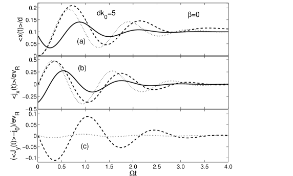
Figure 1: Here $\langle x(t)\rangle/d$, $\langle j_{x}(t)\rangle/{ev_{{}_{R}}}$ and $\langle j_{y}(t)-j_{0}\rangle/{ev_{{}_{R}}}$ are plotted as a function of $\Omega t$. In the all the cases we set $\beta=0$ for GaAs/AlGaAs QW. Here, solid line: ($B_{x}=0$, $B_{y}=0$), dotted line: ($B_{x}=1/\sqrt{2}$ T, $B_{y}=1/\sqrt{2}$ T), dashed line: ($B_{x}=6$ T, $B_{y}=8$ T).

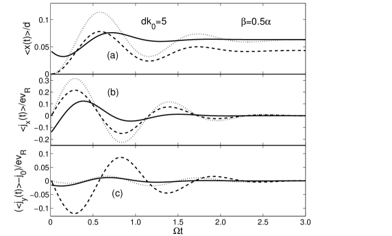
Figure 2: Here $\langle x(t)\rangle/d$, $\langle j_{x}(t)\rangle/{ev_{{}_{R}}}$ and $\langle j_{y}(t)-j_{0}\rangle/{ev_{{}_{R}}}$ are plotted as a function of $\Omega t$. In all the cases we set $\beta=0.5\alpha$ for GaAs/AlGaAs QW. Here, solid line: ($B_{x}=0$, $B_{y}=0$), dotted line: ($B_{x}=1/\sqrt{2}$ T, $B_{y}=1/\sqrt{2}$ T), dashed line: ($B_{x}=6$ T, $B_{y}=8$T).

In Ref. [14] it was shown that the ZB vanishes if $\alpha=\beta$ in the absence of any external magnetic field. But Fig. [3] shows that the ZB is still present when $\alpha=\beta$. This is due to the application of the external in-plane magnetic field.

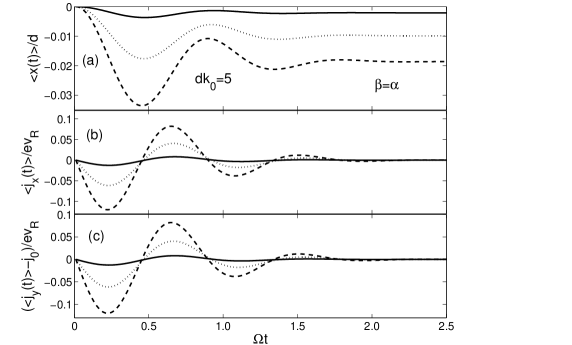
Figure 3: Here $\langle x(t)\rangle/d$, $\langle j_{x}(t)\rangle/{ev_{{}_{R}}}$ and $\langle j_{y}(t)-j_{0}\rangle/{ev_{{}_{R}}}$ are plotted as a function of $\Omega t$. In all the cases we set $\beta=0.5\alpha$ for GaAs/AlGaAs QW. Here, solid line: ($B_{x}=1/\sqrt{2}$ T, $B_{y}=1/\sqrt{2}$ T), dotted line: ($B_{x}=3$ T, $B_{y}=4$ T), dashed line: ($B_{x}=6$ T, $B_{y}=8$ T).

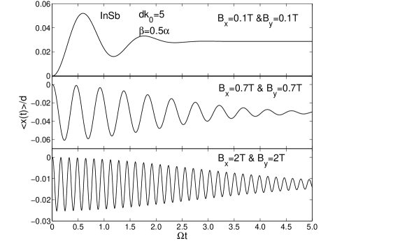
Figure 4: $\langle x(t)\rangle/d$ is plotted as a function of $\Omega t$ for InSb QW. Here, we set $\beta=0.5\alpha$.

InSb QW: Here, we consider InSb QW for which the the effective Lande $g$-factor is very high (e.g $g^{\ast}=-50$) as compared to GaAs/AlGaAs. The RSOI strength is taken to be $\alpha=0.9\times 10^{-11}$ eV-m. We set here $\beta=0.5\alpha$ and $dk_{0}=5$. In Fig. [4] $\langle x(t)\rangle/d$ is plotted with respect to $\Omega t$ for different values of the magnetic field. But the situation is different from the GaAs/AlGaAs QW case. Although the amplitude decreases but the number of oscillations contained in ZB within the same time range is quite large as we increase the magnetic field. Since the magnitude of $g^{\ast}$ is large the coupling between electron’s spin and magnetic field is strong.

One can obtain more oscillation in ZB by increasing the magnitude of the parameter $dk_{0}$ and we have shown that when $dk_{0}>>1$ the pattern is completely oscillatory as evident from Eq.(10). In all these cases it is observed that the ZB is transient in nature i.e it’s amplitude decreases with time and it is a direct consequence of Lock’s lock prediction that the ZB of electron will not be persistent in time if it is represented by a wave packet.

III Zitterbewegung in a Quantum dot

In this section we would like to study ZB of electrons in a semiconductor QD. We consider a 2DEG confined by an isotropic harmonic oscillator potential $V(x,y)=(1/2)m\omega^{2}\big{(}x^{2}+y^{2}\big{)}$. In this context our Hamiltonian reads as

$$H = \frac{p^{2}}{2m}+V(x,y)+\frac{\alpha}{\hbar}\big{(}\sigma_{x}p_{y}-\sigma_{y}p_{x}\big{)}$$ (21)

$$+ \frac{\beta}{\hbar}\big{(}\sigma_{x}p_{x}-\sigma_{y}p_{y}\big{)}+\frac{g^{\ast}}{2}{\mu_{{}_{B}}}\big{(}B_{x}\sigma_{x}+B_{y}\sigma_{y}\big{)}.$$

We introduce the conventional harmonic oscillator creation and annhilation operators as $a_{x}=(x/l+ilp_{x}/\hbar)/\sqrt{2}$, $a_{x}^{\dagger}=(x/l-ilp_{x}/\hbar)/\sqrt{2}$, $a_{y}=(y/l+ilp_{y}/\hbar)/\sqrt{2}$, and $a_{y}^{\dagger}=(y/l-ilp_{y}/\hbar)/\sqrt{2}$, where $l=\sqrt{\hbar/(m\omega)}$ is the harmonic oscillator length.

This Hamiltonian can be re-written as

$$H = \hbar\omega\Big{(}a_{x}^{\dagger}a_{x}+a_{y}^{\dagger}a_{y}+1\Big{)}$$ (22)

$$+ \frac{i\alpha}{\sqrt{2}l}\Big{\{}\big{(}a_{x}-a_{x}^{\dagger}\big{)}\sigma_{y}-\big{(}a_{y}-a_{y}^{\dagger}\big{)}\sigma_{x}\Big{\}}$$

$$+ \frac{i\beta}{\sqrt{2}l}\Big{\{}\big{(}a_{y}-a_{y}^{\dagger}\big{)}\sigma_{y}-\big{(}a_{x}-a_{x}^{\dagger}\big{)}\sigma_{x}\Big{\}}$$

$$+ \frac{g^{\ast}}{2}\mu_{{}_{B}}\big{(}B_{x}\sigma_{x}+B_{y}\sigma_{y}\big{)}.$$

We consider only two lowest occupied energy states (ground state and first excited state) of a two-dimensional harmonic oscillator potential. This approximation is known as the “two sub-band model”. Within this approximation the Hilbert space spanned by the following six basis vectors: $|0,0,\uparrow\rangle$, $|0,0,\downarrow\rangle$, $|1,0,\uparrow\rangle$, $|1,0,\downarrow\rangle$, $|0,1,\uparrow\rangle$, $|0,1,\downarrow\rangle$. Here, $\uparrow$ and $\downarrow$ represent the $z$-component of the electron’s spin vector.

Within six basis vectors one can write the Hamiltonian in a matrix form as

$$H=\begin{pmatrix}H_{11}&H_{12}&0&H_{14}&0&H_{16}\\ H_{21}&H_{22}&H_{23}&0&H_{25}&0\\ 0&H_{32}&H_{33}&H_{34}&0&0\\ H_{41}&0&H_{43}&H_{44}&0&0\\ 0&H_{52}&0&0&H_{55}&H_{56}\\ H_{61}&0&0&0&H_{65}&H_{66}\end{pmatrix}$$

The matrix elements are as follows: $H_{11}=H_{22}=\hbar\omega=\varepsilon_{0}$, $H_{33}=H_{44}=H_{55}=H_{66}=2\hbar\omega=\varepsilon_{1}$, $H_{12}=H_{21}^{\ast}=H_{34}=H_{56}=H_{43}^{\ast}=H_{65}^{\ast}=g^{\ast}\mu_{{}_{B}}\big{(}B_{x}-iB_{y}\big{)}/2$, $H_{14}=H_{41}^{*}=-H_{23}^{*}=-H_{32}=(\alpha-i\beta)/(l\sqrt{2})$, $H_{25}=H_{52}^{*}=-H_{61}=H_{25}^{\ast}=-H_{16}^{*}=-(\beta+i\alpha)/(l\sqrt{2})$.

Here $\varepsilon_{0}=\hbar\omega$ is the zero-point energy and $\varepsilon_{1}=2\hbar\omega$ is the 1st excited state energy of the two-dimensional harmonic oscillator.

We want to determine the expectation value of the time-dependent position operator in this system. Let us consider at $t=0$ the system is in the ground state and the spin is oriented along the positive $z$-direction. This initial state is given by $|\psi(0)\rangle=|0,0,\uparrow\rangle$, so the expectation value of the position operator is given by

$$\langle x_{{}_{H}}(t)\rangle = \langle\psi(0)|x_{{}_{H}}(t)|\psi(0)\rangle$$ (23)

$$= \langle\psi(0)|e^{iHt/\hbar}x(0)e^{-iHt/\hbar}|\psi(0)\rangle$$

$$= \langle 0|VV^{\dagger}e^{iHt/\hbar}VV^{\dagger}xVV^{\dagger}e^{-iHt/\hbar}VV^{\dagger}|0\rangle$$

$$= \langle 0|VV^{\dagger}e^{iHt/\hbar}VXV^{\dagger}e^{-iHt/\hbar}VV^{\dagger}|0\rangle$$

$$= \sum_{i=1}^{6}\Big{(}\sum_{j=1}^{6}V_{j1}H_{ij}e^{i\frac{(\lambda_{i}-\lambda_{j})t}{\hbar}}\Big{)}V_{i1}^{\dagger},$$

where $V$ is the diagonalization matrix which diagonalizes the Hamiltonian $H$ and $VV^{\dagger}=I$. Also, $\omega_{ij}=(\lambda_{i}-\lambda_{j})/\hbar$ is the beating frequency.

The $V$ matrix also diagonalizes $U(t)$ and becomes $U_{diag}(t)=VU(t)V^{\dagger}=e^{-i\lambda_{i}t/\hbar}I_{ij}$ and $X=VxV^{\dagger}$. The position operator is given by $x=\lambda\big{(}a+a^{\dagger}\big{)}/\sqrt{2}$. Within the above mentioned basis this can be written in a matrix form as

$$x=\frac{\lambda}{\sqrt{2}}\begin{pmatrix}0&0&0&0&1&0\\ 0&0&0&0&0&1\\ 0&0&0&0&0&0\\ 0&0&0&0&0&0\\ 1&0&0&0&0&0\\ 0&1&0&0&0&0\end{pmatrix}$$

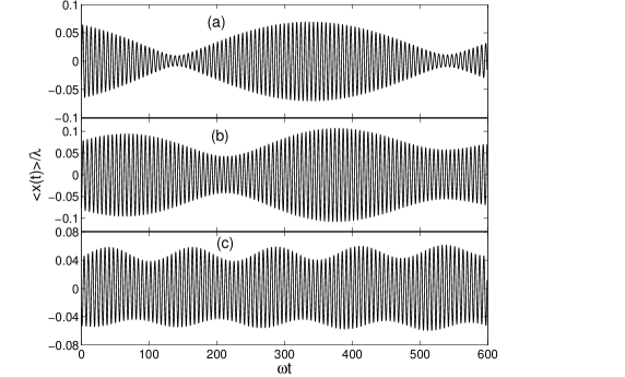
Figure 5: Plots of $\langle x(t)\rangle/\lambda$ vs $\omega t$ for GaAs/AlGaAs QD for different values of magnetic fields. Here, Fig. (a): ($B_{x}=0.1$ T, $B_{y}=0.1$ T), Fig. (b): ($B_{x}=1/\sqrt{(}2)$ T, $B_{y}=1/\sqrt{(}2)$ T), Fig. (c): ($B_{x}=6$ T, $B_{y}=8$ T). We consider only RSOI i.e. $\beta=0$.

III.1 Numerical Results and Discussion

The ZB of a GaAs/AlGaAs quantum dot in the presence of the in-plane magnetic field with SOI is investigated here. The value of the Rashba strength is taken as $\alpha=1.0\times 10^{-11}$ eV-m and the zero-point energy of the harmonic oscillator potential is fixed to the value $\varepsilon_{0}=5$ meV. We find the expectation values of the position coordinate as a function of time which are plotted in Figs. [5] and [6]. In Fig. [5] we fix $\beta=0$ and vary the magnetic field strengths. The magnetic field is kept constant and $\beta$ is varied in Fig. [6]. The ZB in quantum dots is similar to the beating effect in the classical wave mechanics with different frequencies. The oscillatory motion is due to the superposition of individual oscillatory motions with frequencies corresponding to the all possible energy eigenvalue differences of the Hamiltonian. In this case, there are six non-degenerate eigenvalues and we have six values of the energy differences. The number of beating frequencies is six.

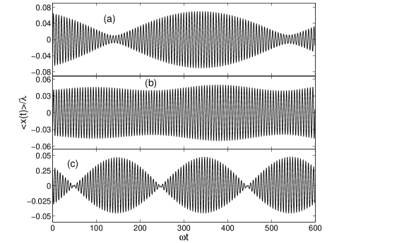
Figure 6: Plots of $\langle x(t)\rangle/\lambda$ vs $\omega t$ for GaAs/AlGaAs QD for different values of $\beta$. The value of magnetic field is kept fixed to $(B_{x},B_{y})=(0.1,0.1)T$. Figures (a),(b) and (c) correspond to $\beta=0$, $\beta=0.5\alpha$ and $\beta=\alpha$ respectively.

IV Conclusion

In this work we have investigated the effect of an external in-plane magnetic field on the ZB of an electron in semiconductor QW and QD with Rashba and Dresselhaus spin-orbit interactions. For QW a general expression of the expectation values of position coordinate and current due to ZB within the Gaussian wave packet is obtained. For QW case, the oscillatory quantum motion of electron which is represented by a wave packet shows transient behavior and this signature is a proof of Lock’s argument. Another important point is that ZB does not vanish even at $\alpha=\beta$ when a finite in-plane magnetic field is present. The $y$-component of current also performs ZB motion with finite magnetic field. We study the same problem for high Lande g-factor QW like InSb in comparison with low Lande g-factor QW like GaAs-AlGaAs. We have also studied the problem of ZB in a GaAs/AlGaAs QD numerically. The ZB in GaAs/AlGaAs QD is persistent in time. The ZB in quantum dots shows beating-like pattern and it is similar to the the beating effect in the classical wave mechanics.

References

• (1) S. Datta and B. Das, Appl. Phys. Lett. 56, 665 (1990).
• (2) I. Zutic, J. Fabian, and S. Das Sarma, Rev. Mod. Phys. 76, 323 (2004).
• (3) S. A. Wolf, et al., Science, 294, 1488 (2002).
• (4) D. D. Awschalom and M. E. Flatte, Nature physics 3, 153 (2007).
• (5) E. I. Rashba, Fiz. Tverd. Tela (Leningrad) 2, 1224 (1960) [Sov. Phys. Solid State 2, 1109 (1960)]; Y. A. Bychkov and E. I. Rashba, J. Phys. C 17, 580 (1984).
• (6) G. Dresselhaus, Phys. Rev. 100, 580 (1955).
• (7) J. Nitta, T. Akazaki, H. Takayanagi, and T. Enoki, Phys. Rev. Lett. 78, 1335 (1997).
• (8) T. Matsuyama, R. Kursten, C. Meibner, and U. Merkt Phys. Rev. B 61, 15588 (2000).
• (9) X. Cartoixa, L. W Wang, D. Z. Y Ting, and Y. C. Chang, Phys. Rev. B 73, 205341 (2006).
• (10) M. H. Liu, K. W. Chen, S. H. Chen, and C.R. Chang, Phys. Rev. B 74, 235322 (2006).
• (11) B. Andrei Bernevig, J. Orenstein, and Shou-Cheng Zhang, Phys. Rev. Lett. 97, 236601 (2006).
• (12) E. Schrodinger, Sitzungsber. Preuss. Akad. Wiss., Phys. Math. Kl. 24, 418 (1930); A. O. Barut and A. J. Bracken, Phys. Rev. D 23, 2454 (1981). (Schrodinger’s original derivation is reproduced here).
• (13) K. Huang, Am. J. Phys. 20, 479 (1952).
• (14) J. A. Lock, Am. J. Phys. 47, 797 (1979).
• (15) W. Zawadzki, Phys. Rev. B 72, 085217 (2005).
• (16) J. Schliemann, D. Loss, and R. M. Westervelt, Phys. Rev. Lett. 94, 206801 (2005).
• (17) J. Schliemann, D Loss, and R M Westervelt, Phys. Rev. B 73, 085323 (2006).
• (18) W. Zawadzki and T. M. Rusin, J. Phys.: Condens. Matter 23, 143201 (2011).
• (19) V. Ya. Demikhovskii, G. M. Maksimova, and E. V. Frolova, Phys. Rev. B 78, 115401 (2008).
• (20) T. M. Rusin and W. Zawadzki, Phys. Rev. B 76, 195439 (2007).
• (21) T. M. Rusin and W. Zawadzki, Phys. Rev. B 78, 125419 (2008).
• (22) G. M. Maksinova, V. Ya. Demikhovskii, and E. V. Frolova, Phys. Rev. B 78, 235321 (2008).
• (23) R. Winkler, U. Zulicke and, J. Bolte, Phys. Rev. B 75, 205314 (2007).
• (24) L. Lamata, J. Leon, T. Schatz, and E. Solano, Phys. Rev. Lett. 98, 253005 (2007).
• (25) R. Gerritsma, G. Kirchmair, F. Zahringer, E. Solano, R. Blatt and, C. F. Roos, Nature 463, 68 (2010).  ̵̈
• (26) J. Y. Vaishnav and W. C. Clark, Phys. Rev. Lett. 100, 153002 (2008); M. Merkl, F. E. Zimmer, G. Juzeliunas, and P. Ohberg, Europhys. Lett. 83, 54002 (2008).
• (27) X. Zhang, Phys. Rev. Lett. 100, 113903 (2008); A. Bermudez, M. A. Martin-Delgado, and A. Luis, Phys. Rev. A 77, 033832 (2008).
• (28) X. Zhang and Z. Liu, Phys. Rev. Lett. 101, 264303 (2008).
• (29) G. David and J. Cserti, Phys. Rev. B 81, 121417(R) (2010).
• (30) B. Vaseghi, G. Rezaei, Z. Moini, S. H. Hendi, and F. Taghizadeh, Superlattices and Microstructure 49, 373 (2011).
• (31) M. C. Chang, Phys. Rev. B 71, 085315 (2005).
• (32) M. Valin-Rodriguez and R. G. Nazmitdinov, Phys. Rev. B 73, 235306 (2006).
• (33) J. Schliemann, J. Carlos Egues, and D. Loss, Phys. Rev. Lett. 90, 146801 (2003).
• (34) J. Schliemann and D. Loss, Phys. Rev. B 68, 165311 (2003).