Levy multiplicative chaos and star scale invariant random measures

Abstract

In this article, we consider the continuous analog of the celebrated Mandelbrot star equation with infinitely divisible weights. Mandelbrot introduced this equation to characterize the law of multiplicative cascades. We show existence and uniqueness of measures satisfying the aforementioned continuous equation. We obtain an explicit characterization of the structure of these measures, which reflects the constraints imposed by the continuous setting. In particular, we show that the continuous equation enjoys some specific properties that do not appear in the discrete star equation. To that purpose, we define a Lévy multiplicative chaos that generalizes the already existing constructions.

, and t3Supported in part by the CHAMU ANR project (ANR-11-JCJC).

60G57, 28A80, 60H25, 60G15, 60G18, Random measure, star equation, scale invariance, multiplicative chaos, uniqueness, infinitely divisible processes, multifractal processes

1 Introduction

Log-normal multiplicative martingales were introduced by Mandelbrot mandelfan in order to build random measures describing energy dissipation and contribute explaining intermittency effects in Kolmogorov’s theory of fully developed turbulence; see cfCastaing , cfSch , cfSto , cfCas , cfFr . Two years later, Mandelbrot mandelbrot introduced the so-called random multiplicative cascades as a more easily understandable and more mathematically tractable alternative. Indeed, this last model was somewhat familiar to the community of turbulence as some authors novikov , yaglom had already considered, with various degrees of rigor, such cascades in the restricted framework of the so called conservative case.

Random multiplicative cascades exhibit nonlinear power-law scalings, rendering intermittency effects in turbulence. Random multiplicative cascades are therefore the first mathematical discrete approach of multifractality. Roughly speaking, a (dyadic) multiplicative cascade is a positive random measure $M$ on the unit interval $[0,1]$ that obeys the following decomposition rule:

$$M(dt)\stackrel{{\scriptstyle\mathrm{law}}}{{=}}Z^{0}\mathbf{1}_{[0,1/2]}(t)M^{0}(2dt)+Z^{1}\mathbf{1}_{[1/2,1]}(t)M^{1}(2dt-1),$$ (1)

where $M^{0},M^{1}$ are two independent copies of $M$, and $(Z^{0},Z^{1})$ is a random vector with prescribed law and positive components of mean $1$ independent from $M^{0},M^{1}$. Such an equation (and its generalizations to $b$-adic trees for $b\geq 2$), the celebrated star equation introduced by Mandelbrot in mandelbrotstar , uniquely determines the law of the multiplicative cascade. Since the seminal work of Mandelbrot, the star equation (1) has been intensively studied: of particular interest are the founding paper by Kahane and Peyriere cfKahPey and the work by Durrett and Ligget durrett . The following literature on the topic essentially builds on these two works. Let us also mention the article Comets which shows that the free energy of a directed polymer model can be obtained as the limit of the free energy of multiplicative cascade models, thus establishing a link between the two models.

Despite the fact that multiplicative cascades have been widely used as reference models in many applications, they possess many drawbacks related to their discrete scale invariance; mainly they involve a particular scale ratio, and they do not possess stationary fluctuations (this comes from the fact that they are constructed on a dyadic tree structure).

Much effort has been made to develop a continuous parameter theory of suitable stationary multifractal random measures ever since, stemming from the theory of multiplicative chaos introduced by Kahane cfKah , Bar , cfSch , bacry , cfRoVa , rhovar . Nevertheless, in comparison with the discrete case, the state of the art concerning continuous time models sounds rather empty: laying the foundations like defining a proper continuous star equation is very recent and its solving only concerns the lognormal situation allez . The main reasons are technical: first, Gaussian processes are very well understood and, second, the analysis of Gaussian multiplicative chaos is much simplified by the use of convexity inequalities for lognormal weights introduced by Kahane; see Kahane’s original paper cfKah or allez , Lemma 10, for instance.

In this paper, we are concerned with solving the continuous star equation:

A stationary random measure $M$ on $\mathbb{R}^{d}$ is said to be $\star$-scale invariant if for all $0<\epsilon\leq 1$, $M$ obeys the cascading rule

$$\bigl{(}M(A)\bigr{)}_{A\in\mathcal{B}(\mathbb{R}^{d})}\stackrel{{\scriptstyle\mathrm{law}}}{{=}}\biggl{(}\int_{A}e^{\omega_{\epsilon}(r)}M^{\epsilon}(dr)\biggr{)}_{A\in\mathcal{B}(\mathbb{R}^{d})},$$ (2)

where $\omega_{\epsilon}$ is a stochastically continuous stationary process and $M^{\epsilon}$ is a random measure independent from $\omega_{\epsilon}$ satisfying the relation

$$\bigl{(}M^{\epsilon}(\epsilon A)\bigr{)}_{A\in\mathcal{B}(\mathbb{R}^{d})}\stackrel{{\scriptstyle\mathrm{law}}}{{=}}\epsilon^{d}\bigl{(}M(A)\bigr{)}_{A\in\mathcal{B}(\mathbb{R}^{d})}.$$

Intuitively, this relation means that when you zoom in the measure $M$, you should observe the same behavior up to an independent factor. Notice that this definition is stated in great generality since no constraint on the law of $\omega_{\epsilon}$ is imposed. In the context of discrete multiplicative cascades, given any law for $\omega_{\epsilon}$ (up to some integrability conditions), this equation can be solved. However, the continuous case imposes the following constraint on $\omega_{\epsilon}$:

Lemma 1.

We consider a nontrivial $\star$-scale invariant measure $M$ on $\mathbb{R}^{d}$. We suppose that for some $x$ (and hence all $x$) the family $\epsilon\rightarrow\omega_{\epsilon}(x)$ is continuous in distribution and

$$\mathbb{E}\bigl{[}\bigl{(}M[0,1]^{d}\bigr{)}^{\gamma}\bigr{]}<\infty,\qquad\mathbb{E}\bigl{[}e^{(1+\gamma)\omega_{\epsilon}(x)}\bigr{]}<\infty\qquad\forall\epsilon\leq 1$$

for some $\gamma>0$. Then, for all $\epsilon$, the process $\omega_{\epsilon}$ is infinitely divisible.

Hence, with minimal assumptions on $\omega_{\epsilon}$ and the solution $M$, the process $\omega_{\epsilon}$ is infinitely divisible. In view of the above lemma, we can suppose that the process $\omega_{\epsilon}$ is infinitely divisible: we will make this assumption in the sequel. As suggested by the Gaussian case allez , this naturally leads to the issue of constructing random measures formally defined by

$$M(dx)=e^{L_{x}}\,dx,$$

where the process $L$ is infinitely divisible with logarithmic correlations. We carry out this construction in Section 2, which generalizes already existing such attempts bacry , Bar , fan , rhovar . We call such measures Lévy multiplicative chaos. This construction enables us not only to give nontrivial solutions to (2) (in Section 3) but also to characterize all the solutions to (2) (up to a few additional technical assumptions). These solutions share the property of a specific structure for the law of the process $\omega_{\epsilon}$. This structure reflects the fact that the continuous star equation is far more restrictive than the discrete one (similarly, Lévy processes are in some sense more restrictive than discrete simple random walks which can be considered with any law for the increments).

1.1 Notation

We will use the following notation throughout the paper. $\mathcal{B}(E)$ stands for the Borel $\sigma$-field of a topological space $E$. A random measure $M$ is a random variable taking values into the set of positive Radon measures defined on $\mathcal{B}(\mathbb{R}^{d})$. We will say that $M$ possesses a moment of order $p>0$ if $\mathbb{E}[M(K)^{p}]<+\infty$ for every compact set $K$. A random measure $M$ is said to be stationary if for all $y\in\mathbb{R}^{d}$ the random measures $M(\cdot)$ and $M(y+\cdot)$ have the same law. A stochastic process $(X_{t})_{t\in\mathbb{R}^{d}}$ is said to be stochastically continuous if, for each $t\in\mathbb{R}^{d}$, $X_{t+h}$ converges toward $X_{t}$ in probability when $h$ goes to $0$. We will also use the shortcut ID in place of infinitely divisible. We remind the reader that every stochastically continuous random process admits a measurable version; see borkar , Chapter 6. We will only deal with measurable versions of stochastically continuous process in this paper.

2 Generalized Lévy chaos

This section is devoted to the construction of measures that can formally be written as

$$M(dx)=e^{L_{x}}\,dx,$$

where $L$ is a stationary ID process with a logarithmic spatial dependency. As in the Gaussian case, such a singularity of the spatial structure imposes to construct these measures through a limiting procedure where the singularity has been “cut off.” Hence we will understand these measures as a limit

$$M(dx)=\lim_{\epsilon\to 0}e^{X^{\epsilon}_{x}}\,dx,$$

where $X^{\epsilon}$ is a stationary ID process that converges in some sense toward $L$. The process $X^{\epsilon}$ will basically depend on two parameters: a generator (any stationary ID process) and a rate function. We detail below the construction.

2.1 Generator and rate function

Let $(X_{t})_{t\in\mathbb{R}^{d}}$ be a stochastically continuous stationary ID random process. It follows from maru that $X$ admits a version given by

$$X_{t} = b+\int_{\mathbb{R}^{d}}\cos(t\cdot\lambda)\overline{W}(d\lambda)+\int_{\mathbb{R}^{d}}\sin(t\cdot\lambda)\overline{W}^{\prime}(d\lambda)$$

$${}+\int_{S}f\bigl{(}T_{t}(s)\bigr{)}\bigl{[}\overline{N}(ds)-\bigl{(}1\vee\bigl{|}f\bigl{(}T_{t}(s)\bigr{)}\bigr{|}\bigr{)}^{-1}\theta(ds)\bigr{]},$$

where:

• $b\in\mathbb{R}$;

• $\overline{W},\overline{W}^{\prime},\overline{N}$ are independent;

• $\overline{W},\overline{W}^{\prime}$ are identically distributed centered Gaussian random measures on $\mathbb{R}^{d}$ with covariance kernel given by $\mathbb{E}[\overline{W}(A)\overline{W}(B)]=R(A\cap B)$ for some symmetric positive finite measure $R$ on $(\mathbb{R}^{d},\mathcal{B}(\mathbb{R}^{d}))$;

• $\overline{N}$ is a Poisson random measure on a Borel space $S$ with a $\sigma$-finite intensity measure $\theta$;

• $f\dvtx S\to\mathbb{R}$ is a measurable deterministic function such that

  $$\int_{S}\bigl{(}\bigl{|}f(s)\bigr{|}^{2}\wedge 1\bigr{)}\theta(ds)<+\infty;$$

• $(T_{x})_{x}$ is a measure preserving flow on $(S,\theta)$.

In what follows, we will say that a stochastically continuous ID process is associated with $(S,\overline{W},\overline{W}^{\prime},\overline{N},\theta,R,f,(T_{x})_{x})$ if it is given by (2.1) where all the involved items are defined as described above.

We define the Laplace exponents $\psi$ of $X$ for $p\geq 1$ by

$$\mathbb{E}\bigl{[}e^{q_{1}X_{t_{1}}+\cdots+q_{p}X_{t_{p}}}\bigr{]}=e^{\psi_{t_{1},\ldots,t_{p}}(q_{1},\ldots,q_{p})}$$

for all $(t_{1},\ldots,t_{p})\in(\mathbb{R}^{d})^{p}$ and $q_{1},\ldots,q_{p}\in\mathbb{R}$ such that the above expectation makes sense. For the sake of clarity, $\psi_{0}$ (i.e., the Laplace exponents of $X_{0}$, or equivalently of $X_{t}$ for any $t\in\mathbb{R}^{d}$) will be denoted by $\psi$.

We assume that $X$ possesses a second order exponential moment, and we consider the following generalized covariance function:

$$F(x) = \psi_{0,x}(1,1)-2\psi(1),\qquad x\in\mathbb{R}^{d}.$$ (4)

Assumption 2.

Let $g$ be a nonnegative function in $L^{1}_{\mathrm{loc}}(\mathbb{R}_{+},dy)$ such that

$$\forall x\in\mathbb{R}^{d}\setminus\{0\}\quad\mbox{and}\quad a\geq 1$$

(5)

$$\qquad\int_{a}^{+\infty}\frac{|F(g(u)x)|}{u}\,du\leq\overline{F}\ln_{+}\frac{1}{a|x|}+h(a,x),$$

where $h$ is some bounded continuous function on $\mathbb{R}_{+}\times\mathbb{R}^{d}$ and $\overline{F}$ is some positive constant. The function $g$ will be called rate function.

2.2 Limiting procedure

For any $\epsilon\in\,]0,1[$, we define a new stochastically continuous ID random process:

$$X^{\epsilon}_{t} = b\ln\frac{1}{\epsilon}+\int_{1}^{1/\epsilon}\!\!\!\int_{\mathbb{R}^{d}}\cos\bigl{(}tg(y)\cdot\lambda\bigr{)}W(d\lambda,dy)$$ (7)

$${}+\int_{1}^{1/\epsilon}\!\!\!\int_{\mathbb{R}^{d}}\sin\bigl{(}tg(y)\cdot\lambda\bigr{)}W^{\prime}(d\lambda,dy)$$

$${}+\int_{1}^{1/\epsilon}\!\!\!\int_{S}f\bigl{(}T_{tg(y)}(s)\bigr{)}\biggl{[}N(ds,dy)-\bigl{(}1\vee\bigl{|}f\bigl{(}T_{tg(y)}(s)\bigr{)}\bigr{|}\bigr{)}^{-1}\theta(ds)\frac{dy}{y}\biggr{]},$$

where:

• $W,W^{\prime},N$ are independent;

• $W,W^{\prime}$ are identically distributed centered Gaussian random measures on $\mathbb{R}^{d}\times\mathbb{R}^{*}_{+}$ with covariance kernel $R(d\lambda)\frac{dy}{y}$, that is, $\mathbb{E}[W(A)W(B)]=\int_{A\cap B}R(d\lambda)\frac{dy}{y}$ for any Borel sets $A,B\subset\mathbb{R}^{d}\times\mathbb{R}^{*}_{+}$;

• $N$ is a Poisson random measure on the Borel space $S\times\mathbb{R}^{*}_{+}$ with intensity measure $\theta(ds)\otimes\frac{dy}{y}$;

• $f\dvtx S\to\mathbb{R}$ and $(T_{x})_{x}$ are the same as above.

Clearly, $X^{\epsilon}$ is a stationary ID process. From maru , Theorem 5, it is stochastically continuous. In what follows, we will say that a family $(X^{\epsilon})_{\epsilon}$ of stationary stochastically continuous ID processes is an approximating family associated with $(S,W,W^{\prime},N,\theta,R,f,(T_{x})_{x})$ if it is given by (LABEL:version2) where all the involved items are defined as described above. Notice that the whole law of the processes $(X^{\epsilon})_{\epsilon\in]0,1]}$ can be recovered from the law of the process $X$ introduced in the previous subsection and the rate function $g$. For this reason, the ID process $X$ will be called the generator of the approximating sequence $(X^{\epsilon})_{\epsilon}$ and $g$ the rate function.

We have

$$\forall q\geq 0,\ \forall x\in\mathbb{R}^{d}\qquad\mathbb{E}\bigl{[}e^{qX^{\epsilon}_{x}}\bigr{]}=\mathbb{E}\bigl{[}e^{qX^{\epsilon}_{0}}\bigr{]}=e^{\ln(1/\epsilon)\psi(q)}.$$ (8)

We stress that, in great generality, $\psi$ takes values into $\mathbb{R}_{+}\cup\{+\infty\}$, but it is finite at least for $q\in[0,2]$.

For $\epsilon>0$, we define a random measure

$$\forall A\in\mathcal{B}\bigl{(}\mathbb{R}^{d}\bigr{)}\qquad\widetilde{M}{}^{\epsilon}(A)=\int_{A}e^{X^{\epsilon}_{x}-\psi(1)\ln(1/\epsilon)}\,dx.$$ (9)

Clearly, for each fixed $A$ with finite Lebesgue measure, the family $(\widetilde{M}{}^{\epsilon}(A))_{\epsilon\in]0,1[}$ is a positive martingale. Thus it converges almost surely. We deduce that the family $(\widetilde{M}{}^{\epsilon})_{\epsilon}$ almost surely weakly converges toward a limiting random measure $M$ on $\mathcal{B}(\mathbb{R}^{d})$. This measure will be called Lévy multiplicative chaos associated with $(S,W,W^{\prime},N,\theta,R,f,(T_{x})_{x})$.

2.3 Main properties

By stationarity and the $0-1$ law, we deduce (as in cfKah , rhovar2 ).

Proposition 3.

Either of the following events occurs with probability one:

$$\{M\equiv 0\}\quad\mbox{or}\quad\bigl{\{}\forall B\mbox{ nonempty ball }M(B)>0\bigr{\}}.$$

In the second situation, we will say that the measure $M$ is nondegenerate.

The nondegeneracy is expectedly related to the Laplace exponents of the generator:

Theorem 4

Under Assumption 2, the measure $M$ is nondegenerate as soon as $\psi^{\prime}(1)-\psi(1)<d$.

Corollary 5.

Under Assumption 2 and provided that $\psi^{\prime}(1)-\psi(1)<d$, the measure $M$ almost surely does not possess any atom.

In some particular situations, it can be proved that the condition $\psi^{\prime}(1)-\psi(1)<d$ is optimal; see cfKah , Bar , bacry , for instance. But the situation presented here is far more intricate and it is not optimal in great generality since we only require the correlation structure to be sub-logarithmic (Assumption 2). To illustrate the situation, let us focus on the second order moment. It is well known that, in the particular situations presented in cfKah , Bar , bacry , the measure $M$ admits a second order moment if and only if $\psi(2)<d$. In our case, the situation is not that clear. For instance, choose $\theta$ equal to the Lebesgue measure on $S=\mathbb{R}^{d}$, $\theta$ any Lévy measure on $\mathbb{R}^{d}$ and $R=0$. The flow $(T_{t})_{t}$ is the usual group of translations. Take any positive bounded function $f$ with compact support over $\mathbb{R}^{d}$ and $g(y)=y^{q}$ (for $q\geq 1$). Notice that the associated function $F$ reduces to $0$ for all $x$ such that the supports of $f$ and $T_{x}f$ are disjoint, say for $|x|\geq R$. Then for $a>0$ and $x\in\mathbb{R}^{d}\setminus\{0\}$, we have (where $e_{x}=x/|x|$)

$$\qquad\quad\int_{1}^{+\infty}\frac{F(u^{q}x)}{u}\,du = \int_{|x|^{1/q}}^{+\infty}\frac{F(u^{q}e_{x})}{u}\,du$$

$$\simeq \frac{F(0)}{q}\ln_{+}\frac{1}{|x|}=\frac{\psi(2)-2\psi(1)}{q}\ln_{+}\frac{1}{|x|}\qquad\mbox{as }x\to 0.$$

Hence it can be proved that $M$ admits a second order moment if and only if $\frac{\psi(2)-2\psi(1)}{q}<d$, which is quite a different condition from cfKah , Bar , bacry .

Hence, it appears that the condition $\psi^{\prime}(1)-\psi(1)<d$ should be optimal when the rate function $g$ is “not far” from the function $g(y)=y$. In that spirit, we claim:

Theorem 6

If the measure $M$ admits a moment of order $1+\delta$ for some $\delta>0$, and if the rate function $g$ satisfies $g(y)\leq y$ for $y\geq 1$, then

$$\psi(1+\delta)-(1+\delta)\psi(1)\leq d\delta.$$

In particular $\psi^{\prime}(1)-\psi(1)<d$.

2.4 On possible generalizations

In the spirit of cfKah , it is possible to make the multiplicative chaos act on other measures than the Lebesgue measure. More precisely, choose a Radon measure $\kappa$ on $\mathbb{R}^{d}$ and, for $\epsilon>0$, define the random measure

$$\forall A\in\mathcal{B}\bigl{(}\mathbb{R}^{d}\bigr{)}\qquad\widetilde{M}{}^{\epsilon}(A)=\int_{A}e^{X^{\epsilon}_{x}-\psi(1)\ln(1/\epsilon)}\kappa(dx).$$ (11)

For each fixed $A$ with finite $\kappa$-measure, the family $(\widetilde{M}{}^{\epsilon}(A))_{\epsilon\in]0,1[}$ is a positive martingale once again and therefore converges almost surely. We deduce that the family $(\widetilde{M}{}^{\epsilon})_{\epsilon}$ almost surely weakly converges toward a limiting random measure $M$ on $\mathcal{B}(\mathbb{R}^{d})$. This measure will be called Lévy multiplicative chaos associated with $(S,W,W^{\prime},N,\theta,R,f,(T_{x})_{x})$ and integrating measure $\kappa$.

A $0-1$ law argument shows:

Proposition 7.

Either of the following events occurs with probability one:

$$\{M\equiv 0\}\quad\mbox{or}\quad\bigl{\{}\forall B\mbox{ nonempty ball with }\kappa(B)>0,M(B)>0\bigr{\}}.$$

In the second situation, we will say that the measure $M$ is nondegenerate.

In this case, nondegeneracy results in an intricate way from the structure of the measure $\kappa$ as well as the Laplace exponents of the generator. It seems difficult to state quite generally a result. Nevertheless we can focus on the situation when the structure of $\kappa$ is related to the Euclidean metric in the following way:

Definition 8.

We introduce the set $R_{\alpha}$ of Radon measures $\nu$ on $\mathbb{R}^{d}$ such that: for any nonempty ball $B$ of $\mathbb{R}^{d}$, for any $\varepsilon>0$, there exist $\delta>0,D>0$, and a compact set $K_{\varepsilon}\subset B$ with $\nu(B\setminus K_{\varepsilon})<\varepsilon$ such that the measure $\nu_{\varepsilon}=\mathbf{1}_{K_{\varepsilon}}(x)\nu(dx)$ satisfies, for every open set $U\subset B$,

$$\nu_{\varepsilon}(U)\leq D\times\operatorname{diam}(U)^{\alpha+\delta}.$$ (12)

In a rough sense, the class $R_{\alpha}$ consists of Radon measures that are locally “$\alpha$-Hölder.” For instance, the Lebesgue measure on $\mathbb{R}^{d}$ is in the class $R_{d}$.

Theorem 9

Under Assumption 2, the measure $M$ is nondegenerate as soon as $\psi^{\prime}(1)-\psi(1)<\alpha$.

Corollary 10.

Under Assumption 2 and provided that $\psi^{\prime}(1)-\psi(1)<\alpha$, the measure $M$ almost surely does not possess any atom.

3 Star scale invariant random measures

In this section, we explain the connection between $\star$-scale invariant random measures and Lévy multiplicative chaos. On one hand, we show that every Lévy multiplicative chaos defines a $\star$-scale invariant random measure provided that the rate function is defined by $g(y)=y$ for all $y\geq 1$. Then we show that all $\star$-scale invariant random measures with a moment of order strictly greater than $1$ are Lévy multiplicative chaos, up to a few additional assumptions.

3.1 Construction

We consider $X^{\epsilon}$, $\widetilde{M}{}^{\epsilon}$ and $M$ as constructed in Section 2 with generator $X$ and rate function $g$ given by $g(y)=y$ for all $y\geq 1$. Hence the process $X^{\epsilon}$ is given by

$$\qquad X^{\epsilon}_{t} = b\ln\frac{1}{\epsilon}+\int_{1}^{1/\epsilon}\!\!\!\int_{\mathbb{R}^{d}}\cos(ty\cdot\lambda)W(d\lambda,dy)$$ (14)

$${}+\int_{1}^{1/\epsilon}\!\!\!\int_{\mathbb{R}^{d}}\sin(ty\cdot\lambda)W^{\prime}(d\lambda,dy)$$

$${}+\int_{1}^{1/\epsilon}\!\!\!\int_{S}f\bigl{(}T_{ty}(s)\bigr{)}\biggl{[}N(ds,dy)-\bigl{(}1\vee\bigl{|}f\bigl{(}T_{ty}(s)\bigr{)}\bigr{|}\bigr{)}^{-1}\theta(ds)\frac{dy}{y}\biggr{]}.$$

Let us state a simple criterion to check Assumption 2:

Proposition 11.

Assumption 2 is satisfied if and only if

$$\sup_{|e|=1}\int_{1}^{+\infty}\frac{|F(ue)|}{u}\,du<+\infty.$$ (15)

Theorem 12

Assume that Assumption 2 [or equivalently (15)] holds and that $\psi^{\prime}(1)-\psi(1)<d$. Then $M$ is nontrivial and $\star$-scale invariant.

Hence, the $\star$-scale invariance property only depends on the choice of the rate function. This shows in a way that there are as many $\star$-scale invariant random measures as stochastically continuous ID processes [up to the condition $\psi^{\prime}(1)-\psi(1)<d$].

The existence of a second order moment is ruled by the following condition, which seems to be more conventional than the counter-example described in (2.3):

Proposition 13.

The measure $M$ admits a second order moment if and only if $F(0)<d$.

A straightforward adaptation of our proofs shows the following:

Proposition 14.

A $\star$-scale invariant random measure $M$ is multifractal in the sense that

$$\lim_{t\downarrow 0}\frac{\ln\mathbb{E}[M([0,t])^{q}]}{\ln t}=q-\psi(q)+q\psi(1),$$

where $\psi$ is the Laplace exponent of its generator.

3.2 Uniqueness

Conversely, we now want to describe as exhaustively as possible the set of all $\star$-scale invariant random measures. For that purpose, we introduce a few additional assumptions:

Assumption 15.

We will say that a stationary random measure $M$ is a good $\star$-scale invariant random measure if $M$ is $\star$-scale invariant and satisfies: [(2)]

the process $\omega_{\epsilon}$ admits exponential moments of order $2$, that is,$\mathbb{E}[e^{2\omega_{\epsilon}(0)}]<\infty$;

for $\epsilon<1$, the generalized covariance kernel associated with the ID process $\omega_{\epsilon}$

$$\forall x\in\mathbb{R}^{d}\qquad F_{\epsilon}(x)=\log\bigl{(}\mathbb{E}\bigl{[}e^{\omega_{\epsilon}(x)+\omega_{\epsilon}(0)}\bigr{]}\bigr{)}$$

satisfies

$$\forall x\neq 0\qquad\bigl{|}F_{\epsilon}(x)\bigr{|}\leq C_{\epsilon}\int_{|x|}^{+\infty}\theta(u)\,du$$ (16)

for some positive constant $C_{\epsilon}$ and some decreasing function $\theta\dvtx]0,+\infty[\,\to\mathbb{R}_{+}$ such that

$$\int_{1}^{+\infty}\theta(u)\ln(u)\,du<+\infty;$$ (17)

there is $\epsilon_{0}\in\,]0,1]$ such that, for each $p\geq 1$, $q_{1},\ldots,q_{p}\in\mathbb{R}$ and $t_{1},\ldots,t_{p}\in\mathbb{R}^{p}$, the mapping

$$(\epsilon,t_{1},\ldots,t_{p})\mapsto\mathbb{E}\bigl{[}e^{iq_{1}\omega_{\epsilon}(t_{1})+i\omega_{\epsilon}(t_{p})}\bigr{]}$$

admits a partial derivative w.r.t. $\epsilon$ at $\epsilon=\epsilon_{0}$ with a partial derivative continuous w.r.t. $(t_{1},\ldots,t_{p})$.

It turns out that the condition on the exponential moments of order $2$ of $\omega_{\epsilon}$ is also necessary as soon as the measure $M$ possesses a moment of order $2$. Point 2 is a decorrelation property at infinity whereas point 3 is a regularity property. In what follows, we denote by $\psi_{\epsilon}$ the Laplace exponent of $\omega_{\epsilon}$,

$$\psi_{\epsilon}(q)=\ln\mathbb{E}\bigl{[}e^{q\omega_{\epsilon}(0)}\bigr{]}$$

for all $q\in\mathbb{R}$ such that the above quantity is finite. Notice that, as soon as the measure $M$ possesses a moment of order $1$, the condition $\psi_{\epsilon}(1)=0$ is a necessary condition for the solution of (2) to be nontrivial.

The main result of this paper is the following:

Theorem 16

Consider a good $\star$-scale invariant measure $M$. Assume that $M$ admits a finite moment of order $1+\delta$ for some $\delta>0$(i.e., $\mathbb{E}[M(B)^{1+\delta}]<\infty$ for some open ball $B$). Then there exists a random variable $Y\in L^{1+\delta}$ and a Lévy multiplicative chaos $Q$ (independent from $Y$ and nondegenerate) with associated rate function $g(y)=y$ such that

$$M(dx)\stackrel{{\scriptstyle\mathrm{law}}}{{=}}YQ(dx).$$

We conjecture that the same theorem holds if $M$ is a $\star$-scale invariant measure with a finite moment of order $1+\delta$ for some $\delta>0$. Therefore, we think Assumption 15 is just a technical assumption (which we cannot avoid at present) and that our theorem characterizes all $\star$-scale invariant measure with a finite moment of order $1+\delta$ for some $\delta>0$. The general case of $\star$-scale invariant measures with no finite moment assumption is currently under investigation and requires the introduction of a different set of measures (work in progress).

Remark 17.

When $M$ is a good $\star$-scale invariant random measure, the law of $M$ is entirely characterized by the law of the process $\omega_{\epsilon}$ in (2) for some $\epsilon\in\,]0,1[$. Furthermore, the law of the finite-dimensional distributions of the generator $X$ can be recovered from those of $\omega_{\epsilon}$ by the following procedure: define the Lévy exponents $\eta^{\epsilon}$, $\eta$ of $\omega_{\epsilon}$ and $X$, that is,

$$\mathbb{E}\bigl{[}e^{iq_{1}\omega_{\epsilon}(t_{1})+\cdots+iq_{p}\omega_{\epsilon}(t_{p})}\bigr{]} = e^{\eta^{\epsilon}(q_{1},\ldots,q_{p},t_{1},\ldots,t_{p})},$$

$$\mathbb{E}\bigl{[}e^{iq_{1}X_{t_{1}}+\cdots+iq_{p}X_{t_{p}}}\bigr{]} = e^{\eta(q_{1},\ldots,q_{p},t_{1},\ldots,t_{p})}.$$

Then we have

$$\partial_{\epsilon}\eta^{\epsilon}(q_{1},\ldots,q_{p},t_{1},\ldots,t_{p})=-\frac{1}{\epsilon^{2}}\eta\biggl{(}q_{1},\ldots,q_{p},\frac{t_{1}}{\epsilon},\ldots,\frac{t_{p}}{\epsilon}\biggr{)}.$$

4 Examples

4.1 Lognormal case

The lognormal case, that is, when the generator of the $\star$-scale invariant measure is a Gaussian process, has been entirely treated in allez . Of course, the assumptions are less restrictive concerning good $\star$-scale invariant measures since their generator can be entirely described with its two marginals, that is its covariance function. As a consequence, we do not require Assumption 15, point (3) in the lognormal case.

4.2 Reminder about log-ID independently scattered random measures

The next examples are based on log-ID independently scattered random measures so that we first collect a few well-known facts about these measures. The reader is referred to rosinski for further details.

We remind the reader that an ID independently scattered random measure $\mu$ distributed on a measurable space $(S,\mathcal{B}(S))$ with control measure $\Gamma$ and kernel $K$ is a collection of random variables $(\mu(A),A\in\mathcal{B}(S))$ such that: [(2)]

for every sequence of disjoint sets $(A_{n})_{n}$ in $\mathcal{B}(S)$, the random variables $(\mu(A_{n}))_{n}$ are independent and

$$\mu\biggl{(}\bigcup_{n}A_{n}\biggr{)}=\sum_{n}\mu(A_{n})\qquad\mbox{a.s.};$$

for any measurable set $A$ in $\mathcal{B}(S)$, $\mu(A)$ is an ID random variable whose characteristic function is characterized by

$$\mathbb{E}\bigl{(}e^{iq\mu(A)}\bigr{)}=\mathbb{E}\bigl{[}e^{it\mu(A)}\bigr{]}=\exp\biggl{(}\int_{A}K(q,s)\Gamma(ds)\biggr{)}.$$

The control measure $\Gamma$ is a positive $\sigma$-finite measure on $S$ and the kernel $K$ takes on the form

$$K(q,s)=iqa(s)-\frac{1}{2}q^{2}\sigma^{2}(s)+\int_{\mathbb{R}}\bigl{(}e^{iqz}-1-iq\tau(z)\bigr{)}\varrho(s,dz),$$ (18)

where

$$\bigl{|}a(s)\bigr{|}+\sigma^{2}(s)+\int_{\mathbb{R}}\min\bigl{(}1,z^{2}\bigr{)}\varrho(s,dz)=1\qquad\theta\mbox{ a.e.}$$ (19)

Here $\sigma,a$ belong to $L^{\infty}(S,\Gamma)$ ($\sigma$ nonnegative) and $\varrho\dvtx S\times\mathcal{B}(\mathbb{R})\to[0,+\infty]$ is such that for each fixed $s\in S$, $\varrho(s,dz)$ is a Lévy measure on $\mathbb{R}$ and for each $B\in\mathcal{B}(\mathbb{R})$ the function $\varrho(\cdot,B)$ is measurable and finite whenever $0$ does not belong to the closure of $B$. The function $\tau$ is any truncation function. The random measure $\mu$ is characterized by the triple of measures $(a(s)\theta(ds),\sigma^{2}(s)\theta(ds),\varrho(s,dz)\theta(ds))$. Conversely, to such triple corresponds a unique (in law) ID independently scattered random measure.

4.3 Barral–Mandelbrot’s type $\star$-scale invariant MRMs

We consider the situation when the dimension $d$ is equal to $1$. We introduce an ID independently scattered random measure $\mu$ distributed on $(\mathbb{R}\times\mathbb{R}^{*}_{+},\mathcal{B}(\mathbb{R}\times\mathbb{R}^{*}_{+}))$ with control measure

$$\Gamma(dt,dy)=dty^{-2}\,dy$$

and kernel

$$K\bigl{(}q,(t,y)\bigr{)}=\varphi(q)=imq-\frac{1}{2}\sigma^{2}q^{2}+\int_{\mathbb{R}^{*}}\bigl{(}e^{iqx}-1-iqx\mathbf{1}_{|x|\leq 1}\bigr{)}\nu(dx),$$

where $\nu(dx)$ is a Lévy measure on $\mathbb{R}$ and $m,\sigma\in\mathbb{R}$. We denote by $\psi$ the Laplace exponent associated with $\varphi$, that is $\psi(q)=\varphi(-iq)$ whenever it makes sense to consider such a quantity. We assume that $\psi(1)=0$.

We can then define the stationary stochastically continuous ID process $(\omega_{l}(t))_{t\in\mathbb{R}}$ for $l>0$ by

$$\omega_{l}(t)=\mu\bigl{(}\mathcal{A}_{l}(t)\bigr{)},$$

where $\mathcal{A}_{l}(t)$ is the triangle like subset $\mathcal{A}_{l}(t)=\{(s,y)\in\mathbb{R}\times\mathbb{R}^{*}_{+}\dvtx l\leq y\leq T,-y/2\leq t-s\leq y/2\}$, see Figure 1.

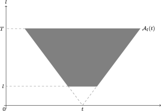
Figure 1: Triangle like subset $\mathcal{A}_{l}(t)$.

Define now the random measure $M_{l}$ by $M_{l}(dt)=e^{\omega_{l}(t)}\,dt$. Almost surely, the family of measures $(M_{l}(dt))_{l>0}$ weakly converges toward a random measure $M$. When $\psi^{\prime}(1)-\psi(1)<1$, this measure is not trivial; see bacry , Bar .

Let us check that $M$ is a good $\star$-scale invariant random measure. Fix $\epsilon<1$, and define the sets $\mathcal{A}_{l,\epsilon T}(t)=\{(s,y)\dvtx l\leq y\leq\epsilon T,-y/2\leq t-s\leq y/2\}$ and $\mathcal{A}_{\epsilon T,T}(t)=\{(s,y)\dvtx\epsilon T\leq y\leq T,-y/2\leq t-s\leq y/2\}$. Note that $\mathcal{A}_{l}(t)=\mathcal{A}_{l,\epsilon T}(t)\cup\mathcal{A}_{\epsilon T,T}(t)$ and that those two sets are disjoint, see Figure 2. Thus we can write for every measurable set $A$

$$M_{l}(A)=\int_{A}e^{\omega_{\epsilon T,T}(t)}e^{\omega_{l,\epsilon T}(t)}\,dt$$ (20)

with $\omega_{\epsilon T,T}(t)=\mu(\mathcal{A}_{\epsilon T,T}(t))$ and $\omega_{l,\epsilon T}(t)=\mu(\mathcal{A}_{l,\epsilon T}(t))$.

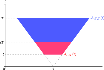
Figure 2: Construction of the sets $\mathcal{A}_{\epsilon T,T}(t)$ and $\mathcal{A}_{l,\epsilon T}(t)$.

We then study equation (20) in the limit $l\to 0$; we obtain

$$M(A)=\int_{A}e^{\omega_{\epsilon T,T}(t)}M^{\epsilon}(dt),$$ (21)

where $M^{\epsilon}$ is the limit when $l\to 0$ of the random measure $M^{\epsilon}_{l}(dt)=e^{\omega_{l,\epsilon T}(t)}\,dt$. We easily verify that $M^{\epsilon}(\epsilon A)\stackrel{{\scriptstyle\mathrm{law}}}{{=}}\epsilon M(A)$ writing

$$M^{\epsilon}_{l}(\epsilon A)=\epsilon\int_{A}e^{\omega_{l,\epsilon T}(\epsilon t)}\,dt$$ (22)

and checking that the finite-dimensional marginals of the process $(\omega_{l,\epsilon T}(\epsilon t))_{t\in\mathbb{R}}$ are the same as the one of $(\omega_{l,T}(t))_{t\in\mathbb{R}}$; see Bar .

By computing the Lévy exponents of the process $\omega_{\epsilon T,T}(t)$,

$$\mathbb{E}\bigl{[}e^{iq_{1}\omega_{\epsilon T,T}(t_{1})+\cdots+iq_{p}\omega_{\epsilon T,T}(t_{p})}\bigr{]}=e^{\psi^{\epsilon}(q_{1},\ldots,q_{p},t_{1},\ldots,t_{p})},$$ (23)

we obtain

$$\psi^{\epsilon}(q_{1},\ldots,q_{p},t_{1},\ldots,t_{p})=\int_{1}^{1/\epsilon}\!\!\!\int_{\mathbb{R}}\varphi\Biggl{(}\sum_{j=1}^{p}q_{j}f\bigl{(}T_{yt_{j}}(r)\bigr{)}\Biggr{)}\,dr\frac{dy}{y},$$ (24)

where $f(r)=\mathbf{1}_{[-T/2,T/2]}(r)$ and $T_{s}\dvtx t\in\mathbb{R}\mapsto t-s\in\mathbb{R}$ is the usual shift on $\mathbb{R}$. It is then straightforward to check that $M$ is good provided that $\int_{z>1}e^{2z}\nu(dz)<+\infty$. We stress that the Lévy exponents of the generator, say $X$, are given by

$$\mathbb{E}\bigl{[}e^{iq_{1}X(t_{1})+\cdots+iq_{p}X(t_{p})}\bigr{]}=\exp\Biggl{(}\int_{\mathbb{R}}\varphi\Biggl{(}\sum_{j=1}^{p}q_{j}f\bigl{(}T_{t_{j}}(r)\bigr{)}\Biggr{)}\,dr\Biggr{)}.$$

In this example, the $\star$-scale invariance property is easily understood via the geometric properties of the process, namely the scaling properties of the cones. Generalizing this example by means of geometric considerations is far from being obvious and has never been done in the literature. On the other hand, in view of the results in this paper, the generalization is straightforward. It suffices to change the function $f$. To make things more simple, we can, for instance, choose $f$ equal to any measurable function bounded by $1$ with compact support.

4.4 Stable Lévy chaos

We focus now on other situations of interest. We consider an infinitely divisible independently scattered random measure $\mu$ distributed on $\mathbb{R}$ with the Lebesgue measure $ds$ as control measure and kernel

$$K(q,t)=\varphi(q)=imq+\int_{0}^{\infty}\bigl{(}e^{-iqx}-1\bigr{)}\frac{dx}{x^{1+\alpha}}$$

for some $\alpha\in\,]0,1[$. Then the associated Laplace exponent is given by

$$\forall q\geq 0\qquad\psi(q)=mq-\frac{\Gamma(1-\alpha)}{\alpha}q^{\alpha}.$$

Let $(T_{t})_{t\in\mathbb{R}}$ be the family of usual shifts on $\mathbb{R}$. Let $f\dvtx\mathbb{R}\to\mathbb{R}_{+}$ be any integrable function with compact support. We define

$$\|f\|_{1}=\int_{\mathbb{R}}f(s)\,ds<+\infty,\qquad\|f\|_{\alpha}=\int_{\mathbb{R}}f(s)^{\alpha}ds<+\infty.$$

We consider the stationary ID random process

$$\forall t\in\mathbb{R}\qquad X_{t}=\int f\bigl{(}T_{t}(s)\bigr{)}\mu(ds).$$

We have

$$\mathbb{E}\bigl{[}e^{qX_{t}}\bigr{]}=e^{\int_{\mathbb{R}}\psi(qf(s))\,ds}=e^{mq\|f\|_{1}-(\Gamma(1-\alpha)/\alpha)\|f\|_{\alpha}q^{\alpha}}.$$

So we must set $m=\frac{\Gamma(1-\alpha)\|f\|_{\alpha}}{\alpha\|f\|_{1}}$ to ensure the normalizing condition $\psi(1)=0$. It is obvious to check that $X$ possesses exponential moments of second order. We assume that $\psi^{\prime}(1)<1$, that is,

$$\|f\|_{\alpha}<\frac{\alpha}{\Gamma(2-\alpha)}.$$

If we consider the Lévy multiplicative chaos with generator $X$ and rate function $g(y)=y$, we obtain a nontrivial good star scale invariant random measure. The scaling factor $\omega_{\epsilon}$ appearing in (2) is a stable ID process.

If we consider the Lévy multiplicative chaos with generator $X$ with $f(x)=\mathbf{1}_{B(x,r)}$ ($B(x,r)$ stands for the ball of radius $r$ centered at $x$) and rate function $g(y)=\sum_{n\geq 0}n\mathbf{1}_{[n,n+1[}(y)$, we recover Fan’s stable Lévy chaos.

5 Conjectures and open problems

5.1 Convergence of the derivative martingale

Consider a Lévy multiplicative chaos on $\mathbb{R}^{d}$ with integrating measure the Lebesgue measure. Let $\psi$ be the Laplace exponent to its generator and $(X^{\epsilon})_{\epsilon}$ the associated approximating family. Consider the martingale

$$M_{\epsilon}^{\theta}(dx)=\int_{\cdot}e^{\theta X_{\epsilon}(x)-\psi(\theta)\ln(1/\epsilon)}\,dx.$$ (25)

For $\theta\in\mathbb{R}_{+}$, define the function

$$\forall q\in\mathbb{R}\qquad\xi_{\theta}(q)=\bigl{(}d+\psi(\theta)\bigr{)}q-\psi(q\theta).$$

There is at most one solution $\theta_{0}>0$ to the equation $\xi^{\prime}_{\theta}(1)=0$.

Let us discuss the (only nontrivial) situation when $0<\theta_{0}<\infty$. The nondegeneracy condition of Theorem 4 reads $\xi^{\prime}_{\theta}(1)>0$, and it is valid if and only if $\theta<\theta_{0}$. Inspired by the Gaussian case (see cfKah ) or multiplicative cascades (see cfKahPey ), prove the following:

Conjecture 18.

For $\theta\geq\theta_{0}$, the martingale defined by (25) converges almost surely toward $0$.

Deduce the following estimate for the statistics of the maximum of a log-correlated infinitely divisible process:

Conjecture 19.

For any open bounded set $A$, we have

$$\max_{x\in A}X_{\epsilon}(x)-\psi^{\prime}(\theta_{0})\ln\frac{1}{\epsilon}\to-\infty\qquad\mbox{as }\epsilon\to 0.$$

At the critical point $\theta=\theta_{0}$, we must introduce the so-called derivative martingale (see Rnew7 )

$$D_{\epsilon}^{\theta}(dx)=\int_{\cdot}\biggl{(}\psi(\theta_{0})\ln\frac{1}{\epsilon}-X_{\epsilon}(x)\biggr{)}e^{\theta_{0}X_{\epsilon}(x)-\psi(\theta_{0})\ln(1/\epsilon)}\,dx.$$ (26)

Conjecture 20.

Prove that the derivative martingale almost surely converges toward a nontrivial positive random measure, denoted by $M^{\prime}$. Prove that $M^{\prime}$ does not possess atoms.

Conjecture 21.

Prove that the derivative martingale can be obtained as a suitable renormalization of the sequence $(M^{\theta_{0}}_{\epsilon})_{\epsilon}$. More precisely,

$$\sqrt{\ln\frac{1}{\epsilon}}M^{\theta_{0}}_{\epsilon}(dx)\to cM^{\prime}(dx)\qquad\mbox{as }\epsilon\to 0$$

for some deterministic factor $c$.

5.2 Conjectures about star scale invariance

Consider the star scale invariance equation in great generality, that is:

Definition 22 ((Star scale invariance)).

A random Radon measure $M$ is star scale invariant if for all $0<\epsilon\leq 1$, $M$ obeys the cascading rule

$$\bigl{(}M(A)\bigr{)}_{A\in\mathcal{B}(\mathbb{R}^{d})}\stackrel{{\scriptstyle\mathrm{law}}}{{=}}\biggl{(}\int_{A}e^{\omega_{\epsilon}(r)}M^{\epsilon}(dr)\biggr{)}_{A\in\mathcal{B}(\mathbb{R}^{d})},$$ (27)

where $\omega_{\varepsilon}$ is a stationary stochastically continuous Gaussian process, and $M^{\varepsilon}$ is a random measure independent from $\omega_{\varepsilon}$ satisfying the scaling relation

$$\bigl{(}M^{\epsilon}(A)\bigr{)}_{A\in\mathcal{B}(\mathbb{R}^{d})}\stackrel{{\scriptstyle\mathrm{law}}}{{=}}\biggl{(}M\biggl{(}\frac{A}{\epsilon}\biggr{)}\biggr{)}_{A\in\mathcal{B}(\mathbb{R}^{d})}.$$ (28)

Observe that the main difference with (2) is that we do not impose here the normalization $\mathbb{E}[e^{\omega_{\epsilon}(r)}]=\epsilon^{d}$. As soon as the measure possesses a moment of order $1+\delta$ for some $\delta>0$, the condition $\mathbb{E}[e^{\omega_{\epsilon}(r)}]=\epsilon^{d}$ must be satisfied. So it remains to investigate situations when the measure possesses moments of at most order $1$.

Inspired by the discrete multiplicative cascade case (see durrett ), we conjecture:

Conjecture 23.

Prove that, if $M$ is a good star scale invariant measure, there exists a $\alpha\in\,]0,1]$ such that

$$\mathbb{E}\bigl{[}e^{\alpha\omega_{\epsilon}(r)}\bigr{]}=\epsilon^{d}.$$

Assuming this, we may follow the proof of Theorem 16 to see that the process $\alpha\omega_{\epsilon}$ has a structure given by (LABEL:version2). More precisely, we can then rewrite the process $\omega_{\epsilon}$ as

$$\omega_{\epsilon}(x)=\frac{1}{\alpha}X_{\epsilon}(x)-\frac{\psi(1)}{\alpha}\ln\frac{1}{\epsilon}-\frac{d}{\alpha}\ln\frac{1}{\epsilon}$$ (29)

for some family $(X_{\epsilon})_{\epsilon}$ of the type (LABEL:version2), and $\psi$ is its Laplace exponent.

Conjecture 24.

Assume that $M$ is an ergodic good star scale invariant measure, and let (29) be the decomposition of $\omega_{\epsilon}$: [(3)]

If $\alpha=1$ and $\psi^{\prime}(1)-\psi(1)<d$, then the law of the solution $M$ is Levy multiplicative chaos multiplicative chaos with rate function $g(y)=y$ up to a deterministic multiplicative constant; see Theorem 16.

If $\alpha=1$ and $\psi^{\prime}(1)-\psi(1)=d$, prove that the law of the solution $M$ is that of the limit of the derivative martingale, namely $M^{\prime}$ described above, up to a multiplicative constant.

If $\alpha<1$ and $\psi^{\prime}(1)-\psi(1)<d$, prove that $M$ is an “atomic Lévy multiplicative chaos” (see Rnew4 in the Gaussian case) up to a multiplicative constant. More precisely, the law can be constructed as follows:

1. [(a)]

2. Sample the standard Levy multiplicative chaos

   $$\overline{M}(dx)=\lim_{\epsilon\to 0}\int_{\cdot}e^{X_{\epsilon}(x)-\psi(1)\ln(1/\epsilon)}\,dx.$$

   The measure $\overline{M}$ is perfectly defined since $\psi^{\prime}(1)-\psi(1)<d$.

3. Sample a point process $M$ whose law, conditioned on $\overline{M}$, is that of an independently scattered random measure characterized by

   $$\forall q\geq 0\qquad\mathbb{E}\bigl{[}e^{-qM(A)}|\overline{M}\bigr{]}=e^{-q^{\alpha}\overline{M}(A)}.$$

If $\alpha<1$ and $\psi^{\prime}(1)-\psi(1)=d$, prove that $M$ is an atomic Lévy multiplicative chaos of a second type. More precisely, the law can be constructed as follows:

1. [(a)]

2. sample the derivative Lévy multiplicative chaos $M^{\prime}(dx)$ as described above;

3. sample a point process $M$ whose law, conditioned on $M^{\prime}$, is that of an independently scattered random measure characterized by

   $$\forall A\in\mathcal{B}\bigl{(}\mathbb{R}^{d}\bigr{)},\ \forall q\geq 0\qquad\mathbb{E}\bigl{[}e^{-qM(A)}|M^{\prime}\bigr{]}=e^{-q^{\alpha}M^{\prime}(A)}.$$

The reader may find in Rnew4 , Rnew7 some further conjectures in the Gaussian case that can also be adapted to this framework. In particular, adapting these conjectures to our framework, the reader may deduce conjectures about the glassy phase and freezing phenomena of log-correlated infinitely divisible random potentials and about the asymptotics of the extreme values of log-correlated infinitely divisible random fields.

Appendix A Proof of Lemma 1

We first state the following intermediate lemma:

Lemma 25.

Let $(F(x))_{x\in\mathbb{R}^{d}}$ and $(G(x))_{x\in\mathbb{R}^{d}}$ be two stationary and nonnegative stochastically continuous processes. We consider a nontrivial stationary random measure $\eta$ on $\mathbb{R}^{d}$ independent of $F,G$. We suppose that there exists $\gamma>0$ such that $\mathbb{E}[F(x)^{1+\gamma}]<\infty$, $\mathbb{E}[G(x)^{1+\gamma}]<\infty$, and $\mathbb{E}[\eta(K)^{\gamma}]<\infty$ for all compact set $K$. If the following equality on measures holds:

$$F(x)\eta(dx)\stackrel{{\scriptstyle\mathrm{law}}}{{=}}G(x)\eta(dx),$$

then the two processes $F$ and $G$ have same law.

We consider the case $d=1$ (the higher dimensions work the same). Let $\delta>0$. Notice that $\mathbb{E}[\eta([0,\delta])^{\alpha}]>0$ for all $\alpha\in\,]0,\gamma[$. Indeed, the measure is stationary and nontrivial. Choose now $\alpha\in\,]0,\min(\gamma,1)[$. Notice that the mapping $x\in\mathbb{R}_{+}\mapsto x^{\alpha}$ is sub-additive. Therefore $|x^{\alpha}-y^{\alpha}|\leq|x-y|^{\alpha}$ for any $x,y\geq 0$. We deduce the following inequality:

$$\biggl{|}\mathbb{E}\biggl{[}\biggl{(}\int_{0}^{\delta}F(x)\eta(dx)\biggr{)}^{\alpha}\biggr{]}-\mathbb{E}\biggl{[}\biggl{(}\int_{0}^{\delta}F(0)\eta(dx)\biggr{)}^{\alpha}\biggr{]}\biggr{|}$$

$$\qquad\leq\mathbb{E}\biggl{[}\biggl{|}\int_{0}^{\delta}F(x)\eta(dx)-\int_{0}^{\delta}F(0)\eta(dx)\biggr{|}^{\alpha}\biggr{]}$$

$$\qquad\leq\mathbb{E}\biggl{[}\biggl{(}\int_{0}^{\delta}\bigl{|}F(x)-F(0)\bigr{|}\eta(dx)\biggr{)}^{\alpha}\biggr{]}.$$

The mapping $x\in\mathbb{R}_{+}\mapsto x^{\alpha}$ is concave. So we use Jensen’s inequality applied to $\mathbb{E}[\cdot|\eta]$, and we get:

$$\biggl{|}\mathbb{E}\biggl{[}\biggl{(}\int_{0}^{\delta}F(x)\eta(dx)\biggr{)}^{\alpha}\biggr{]}-\mathbb{E}\biggl{[}\biggl{(}\int_{0}^{\delta}F(0)\eta(dx)\biggr{)}^{\alpha}\biggr{]}\biggr{|}$$

$$\qquad\leq\mathbb{E}\biggl{[}\biggl{(}\int_{0}^{\delta}\mathbb{E}\bigl{[}\bigl{|}F(x)-F(0)\bigr{|}\bigr{]}\eta(dx)\biggr{)}^{\alpha}\biggr{]}$$

$$\qquad\leq\sup_{x\in[0,\delta]}\mathbb{E}\bigl{[}\bigl{|}F(x)-F(0)\bigr{|}\bigr{]}^{\alpha}\mathbb{E}\bigl{[}\eta[0,\delta]^{\alpha}\bigr{]}.$$

Since $\sup_{x\in[0,\delta]}\mathbb{E}[|F(x)-F(0)|]\mathop{\rightarrow}\limits_{\delta\to 0}0$, we get that

$$\frac{\mathbb{E}[(\int_{0}^{\delta}F(x)\eta(dx))^{\alpha}]}{\mathbb{E}[\eta[0,\delta]^{\alpha}]}\mathop{\rightarrow}\limits_{\delta\to 0}\mathbb{E}\bigl{[}F(0)^{\alpha}\bigr{]}.$$

Similarly, we get the above convergence with $F$ replaced by $G$: this shows that $F(0)$ and $G(0)$ have the same distribution. We show similarly, for all $x_{1},\ldots,x_{n}$, that $(F(x_{1}),\ldots,F(x_{n}))$ and $(G(x_{1}),\ldots,G(x_{n}))$ have the same distribution.

Now, we can finish the proof of Lemma 1:

Proof of Lemma 1 By iterating (2) and using the above lemma, the process $(\omega_{\epsilon}(x))_{x\in\mathbb{R}^{d}}$ is such that ($\epsilon,\epsilon^{\prime}<1$),

$$\bigl{(}\omega_{\epsilon\epsilon^{\prime}}(x)\bigr{)}_{x\in\mathbb{R}^{d}}\stackrel{{\scriptstyle\mathrm{law}}}{{=}}\biggl{(}\omega_{\epsilon}(x)+\tilde{\omega}_{\epsilon^{\prime}}\biggl{(}\frac{x}{\epsilon}\biggr{)}\biggr{)}_{x\in\mathbb{R}^{d}},$$ (30)

where $\omega_{\epsilon}$ and $\tilde{\omega}_{\epsilon^{\prime}}$ are independent copies of $\omega_{\epsilon}$ and $\omega_{\epsilon^{\prime}}$. We fix $\epsilon$ and consider $\epsilon_{n}={\epsilon}^{1/n}$. Of course $\epsilon_{n}^{n}=\epsilon$. By iterating the cascade rule (30), we get

$$\bigl{(}\omega_{\epsilon}(x)\bigr{)}_{x\in\mathbb{R}^{d}}\stackrel{{\scriptstyle\mathrm{law}}}{{=}}\Biggl{(}\sum_{k=0}^{n-1}\omega_{\epsilon_{n}}^{(k)}\biggl{(}\frac{x}{\epsilon_{n}^{k}}\biggr{)}\Biggr{)}_{x\in\mathbb{R}^{d}},$$

where the $\omega_{\epsilon_{n}}^{(k)}$ are independent processes of law $\omega_{\epsilon_{n}}$. Fix $x,y\in\mathbb{R}^{d}$. We therefore have for all $\lambda,\mu$,

$$\lambda\omega_{\epsilon}(x)+\mu\omega_{\epsilon}(y)\stackrel{{\scriptstyle\mathrm{law}}}{{=}}\sum_{k=0}^{n-1}\mu\omega_{\epsilon_{n}}^{(k)}\biggl{(}\frac{x}{\epsilon_{n}^{k}}\biggr{)}+\lambda\omega_{\epsilon_{n}}^{(k)}\biggl{(}\frac{y}{\epsilon_{n}^{k}}\biggr{)}.$$

The stochastic continuity of the process $\omega$ with respect to $\epsilon$ entails, for all $\eta>0$,

$$\sup_{0\leq k\leq n-1}P\biggl{(}\biggl{|}\mu\omega_{\epsilon_{n}}^{(k)}\biggl{(}\frac{x}{\epsilon_{n}^{k}}\biggr{)}+\lambda\omega_{\epsilon_{n}}^{(k)}\biggl{(}\frac{y}{\epsilon_{n}^{k}}\biggr{)}\biggr{|}>\eta\biggr{)}\mathop{\rightarrow}\limits_{n\to\infty}0.$$

By a classical theorem on independent triangular arrays (see Chapter XVII in Feller ), this shows that the couple $(\omega_{\epsilon}(x),\omega_{\epsilon}(y))$ is ID. One proceeds similarly to show that, for all $(x_{1},\ldots,x_{n})$, the vector $(\omega_{\epsilon}(x_{1}),\ldots,\omega_{\epsilon}(x_{n}))$ is ID.

Appendix B Proof of Theorem 4

We adapt the proofs of cfKah , rhovar .

The class $R_{\alpha}$. Let $B$ be a nonempty ball of $\mathbb{R}^{d}$. We introduce the set $R_{\alpha}$ of Radon measures $\nu$ on $B$ satisfying: for any $\varepsilon>0$, there exist $\delta>0,D>0$ and a compact set $K_{\varepsilon}\subset B$ with $\nu(B\setminus K_{\varepsilon})<\varepsilon$ such that the measure $\nu_{\varepsilon}=\mathbf{1}_{K_{\varepsilon}}(x)\nu(dx)$ satisfies, for every open set $U\subset B$,

$$\nu_{\varepsilon}(U)\leq D\times\operatorname{diam}(U)^{\alpha+\delta}.$$ (31)

We further define the set of Radon measures $R^{\alpha}_{-}=\bigcap_{\beta<\alpha}R^{\beta}$. For a Radon measure $\nu$, we define the quantity

$$C_{\alpha}(\nu)=\int_{B\times B}\frac{1}{|x-y|^{\alpha}}\nu(dx)\nu(dy).$$

It is plain to see that

$$C_{\alpha}(\nu)<\infty\quad\Longrightarrow\quad\nu\in R^{\alpha}_{-}.$$

Conversely, a measure obeying (31) satisfies $C_{\beta}(\nu)<+\infty$ for all $\beta<\alpha+\delta$.

We show the following intermediate result:

Lemma 26.

Consider a Radon measure $\kappa\in R_{\alpha}$. Let $N$ be the Radon measure defined on $B$ by

$$N(dx)=\lim_{\varepsilon\searrow 0}e^{X^{\varepsilon}_{x}-\psi(1)\ln(1/\varepsilon)}\kappa(dx)=:\lim_{\varepsilon\searrow 0}N_{\varepsilon}(dx).$$

If $\overline{F}<\alpha$, then the martingale $(N_{\epsilon}(B))_{\epsilon}$ is regular and $N\in R_{\alpha-\psi^{\prime}(1)+\psi(1)}$.

We first show that the martingale $(N_{\epsilon}(B))_{\epsilon}$ is regular. For this, we use the fact that $F(\cdot)$ verifies Assumption 2 to get (for some positive constant $S=\sup_{\mathbb{R}_{+}\times\mathbb{R}^{d}}|h|$)

$$\mathbb{E}\bigl{[}N_{\epsilon}(B)^{2}\bigr{]} = \int_{B\times B}\mathbb{E}\bigl{[}e^{X_{x}^{\epsilon}+X_{y}^{\epsilon}}\bigr{]}e^{-2\psi(1)\ln(1/\epsilon)}\kappa(dx)\kappa(dy)$$

$$= \int_{B\times B}e^{\int_{1}^{1/\varepsilon}F(g(u)(x-y))((du)/u)}\kappa(dx)\kappa(dy)$$

$$\leq \int_{B\times B}e^{\int_{1}^{\infty}\bigl{|}F(g(u)(x-y))\bigr{|}((du)/u)}\kappa(dx)\kappa(dy)$$

$$\leq \int_{B\times B}e^{\overline{F}\ln_{+}(1/|x-y|)+S}\kappa(dx)\kappa(dy)$$

$$\leq e^{S}\int_{B\times B}\max\biggl{(}\frac{1}{|x-y|^{\overline{F}}},1\biggr{)}\kappa(dx)\kappa(dy)$$

and the last integral is finite as soon as $\overline{F}<\alpha$. Hence, the martingale $(N_{\epsilon}(B))_{\epsilon}$ is regular.

We consider a compact set $K\subset B$. Even if it means multiplying $\kappa$ by a positive constant, we assume that $\kappa(K)=1$. We consider on $\Omega\times K$ the probability measure $\mathbb{Q}$ defined by

$$\int_{\Omega\times K}f(\omega,x)\,d\mathbb{Q}=\mathbb{E}\biggl{[}\int_{K}f(\omega,x)N(dx)\biggr{]},$$

where $f$ is any nonnegative measurable function.

For $0<\varepsilon^{\prime}<\varepsilon<1$, we define the process $(X^{\varepsilon^{\prime},\varepsilon}_{x})_{x\in\mathbb{R}^{d}}$ by

$$\forall x\in\mathbb{R}^{d}\qquad X^{\varepsilon^{\prime},\varepsilon}_{x}=X^{\varepsilon^{\prime}}_{x}-X^{\varepsilon}_{x}-\psi(1)\ln\bigl{(}\varepsilon/\varepsilon^{\prime}\bigr{)}.$$

Because of expression (LABEL:defX), it is straightforward to check that, given $\varepsilon_{1}<\varepsilon_{2}<\cdots<\varepsilon_{n}$, the processes $X^{\varepsilon_{1},\varepsilon_{2}},X^{\varepsilon_{2},\varepsilon_{3}},\ldots,X^{\varepsilon_{n-1},\varepsilon_{n}}$ are $\mathbb{Q}$-independent. Moreover, for $\lambda\geq 0$ and because $(N_{\epsilon})_{\epsilon}$ is uniformly integrable, we have

$$\int e^{\lambda X^{\varepsilon^{\prime},\varepsilon}_{x}}\,d\mathbb{Q}$$

$$\!\!\qquad=\int_{K}\mathbb{E}\biggl{[}\exp\biggl{\{}\lambda\int_{1/\epsilon}^{1/\epsilon^{\prime}}\!\!\!\int_{\mathbb{R}^{d}}\cos\bigl{(}xg(y)\cdot u\bigr{)}W(du,dy)$$

$$\!\!\hskip 79.0pt{}+\sin\bigl{(}xg(y)\cdot u\bigr{)}W^{\prime}(du,dy)+\lambda b\ln\frac{\epsilon}{\epsilon^{\prime}}-\lambda\psi(1)\ln\bigl{(}\varepsilon/\varepsilon^{\prime}\bigr{)}\biggr{\}}$$

$$\!\!\hskip 57.0pt{}\times\exp\biggl{\{}\lambda\int_{1/\epsilon}^{1/\epsilon^{\prime}}\!\!\!\int_{S}f\bigl{(}T_{tg(y)}(s)\bigr{)}$$

$$\!\!\hskip 130.0pt{}\times\biggl{[}N(ds,dy)$$

$$\!\!\hskip 145.0pt{}-\bigl{(}1\vee\bigl{|}f\bigl{(}T_{tg(y)}(s)\bigr{)}\bigr{|}\bigr{)}^{-1}\theta(ds)\frac{dy}{y}\biggr{]}\biggr{\}}$$

$$\!\!\hskip 220.0pt{}\times\exp\biggl{\{}X^{\epsilon^{\prime}}_{x}-\psi(1)\ln\frac{1}{\epsilon^{\prime}}\biggr{\}}\biggr{]}\kappa(dx)$$

$$\!\!\qquad=\int_{K}\mathbb{E}\biggl{[}\exp\biggl{\{}(\lambda+1)\int_{1/\epsilon}^{1/\epsilon^{\prime}}\!\!\!\int_{\mathbb{R}^{d}}\cos\bigl{(}xg(y)\cdot u\bigr{)}W(du,dy)$$

$$\!\!\hskip 80.0pt{}+\sin\bigl{(}xg(y)\cdot u\bigr{)}W^{\prime}(du,dy)+(\lambda+1)b\ln\frac{\epsilon}{\epsilon^{\prime}}$$

$$\!\!\hskip 174.0pt{}-(\lambda+1)\psi(1)\ln\bigl{(}\varepsilon/\varepsilon^{\prime}\bigr{)}\biggr{\}}$$

$$\!\!\hskip 57.0pt{}\times\exp\biggl{\{}(\lambda+1)\int_{1/\epsilon}^{1/\epsilon^{\prime}}\!\!\!\int_{S}f\bigl{(}T_{tg(y)}(s)\bigr{)}$$

$$\!\!\hskip 155.0pt{}\times\biggl{[}N(ds,dy)$$

$$\!\!\hskip 170.0pt{}-\bigl{(}1\vee\bigl{|}f\bigl{(}T_{tg(y)}(s)\bigr{)}\bigr{|}\bigr{)}^{-1}\theta(ds)\frac{dy}{y}\biggr{]}\biggr{\}}\biggr{]}\kappa(dx)$$

$$\!\!\qquad=\exp\biggl{\{}\psi(\lambda+1)\ln\bigl{(}\varepsilon/\varepsilon^{\prime}\bigr{)}-(\lambda+1)\psi(1)\ln\bigl{(}\varepsilon/\varepsilon^{\prime}\bigr{)}\biggr{\}}.$$

In particular, under $\mathbb{Q}$, the process $u\in\mathbb{R}^{+}\mapsto X^{e^{-u},1}$ is an integrable Lévy process. Thus from the strong law of large numbers, we get that $\mathbb{Q}$-almost surely:

$$\frac{X^{e^{-u},1}}{u}\to\psi^{\prime}(1)-\psi(1),$$

when $u\to\infty$. Consequently, $\mathbb{P}$ almost surely,

$$N\mbox{ a.s.},\qquad\frac{X^{e^{-u}}_{x}}{u}\to\psi^{\prime}(1).$$ (32)

In particular, by Egoroff’s theorem, there exists a compact set $K_{\varepsilon}^{1}\subset K$ such that $N(K\setminus K_{\varepsilon}^{1})<\varepsilon$ and the convergence (32) is uniform with respect to $x\in K_{\varepsilon}^{1}$. Let now $q>0$, and define $N_{q}(dy)=\lim_{\epsilon\searrow 0}e^{X^{\epsilon,e^{-q}}_{y}}\kappa(dy)$ and $P_{q}(x)=N_{q}(B_{x}^{q}\cap K)$ where $B_{x}^{q}$ denotes the ball centered on $x$ and with radius $e^{-q}$. We finally define the function

$$\theta_{q}(x,y)=\mathbf{1}_{\{|x-y|\leq e^{-q}\}},$$

in such a way that $P_{q}(x)=\int_{K}\theta_{q}(x,y)N_{q}(dy)$. Thus we have:

$$\int P_{q}\,d\mathbb{Q} = \mathbb{E}\biggl{[}\int_{K\times K}\theta_{q}(x,y)N_{q}(dx)N(dy)\biggr{]}$$

$$= \lim_{\epsilon\to 0}\mathbb{E}\biggl{[}\int_{K\times K}\theta_{q}(x,y)e^{X^{\epsilon,e^{-q}}_{x}+X^{\epsilon,e^{-q}}_{y}}\kappa(dx)\kappa(dy)\biggr{]}$$

$$= \int_{K\times K}\theta_{q}(x,y)e^{\int_{[e^{q},\infty]}F(g(u)(y-x))((du)/u)}\kappa(dx)\kappa(dy).$$

Let $\beta>\overline{F}$ be fixed. By using Assumption 2 and the above relation, we obtain (for some positive constant $S=\sup_{\mathbb{R}_{+}\times\mathbb{R}^{d}}|h|$)

$$\int\sum_{n\geq 1}e^{\beta n}P_{n}\,d\mathbb{Q}$$

$$\qquad=\sum_{n\geq 1}\int_{K\times K}\theta_{n}(x,y)e^{\beta n}e^{\int_{[e^{n},\infty]}F(g(u)(y-x))((du)/u)}\kappa(dx)\kappa(dy)$$

$$\qquad=\int_{K\times K}\sum_{1\leq n\leq-\ln(|x-y|)}e^{\beta n}e^{\int_{[e^{n},\infty]}F(g(u)(y-x))((du)/u)}\kappa(dx)\kappa(dy)$$

$$\qquad\leq e^{S}\int_{K\times K}\sum_{1\leq n\leq-\ln(|x-y|)}e^{\beta n}e^{\overline{F}\ln(1/(e^{n}|x-y|))}\kappa(dx)\kappa(dy)$$

$$\qquad\leq e^{S}\int_{K\times K}\sum_{1\leq n\leq-\ln(|x-y|)}e^{(\beta-\overline{F})n}\frac{1}{|x-y|^{\overline{F}}}\kappa(dx)\kappa(dy).$$

Note that, for some positive constant $D$,

$$\sum_{1\leq n\leq-\ln(|x-y|)}e^{(\beta-\overline{F})n}\leq D\frac{1}{|x-y|^{\beta-\overline{F}}},$$

in such a way that

$$\int\sum_{n\geq 1}e^{\beta n}P_{n}\,d\mathbb{Q} \leq De^{S}\int_{K\times K}\frac{1}{|x-y|^{\beta}}\kappa(dx)\kappa(dy)=DD^{\prime}C_{\beta}(\kappa).$$

The last term is finite as soon as $\beta<\alpha$. Thus for $\beta\in\,]\overline{F},\alpha[$, $\mathbb{Q}$ a.s., $e^{\beta n}P_{n}\to 0$ as $n\to\infty$. In particular, one can find a compact set $K_{\varepsilon}^{2}\subset K$ such that $N(K\setminus K_{\varepsilon}^{2})<\varepsilon$ and such that, $N$ almost surely,

$$\limsup_{n\to\infty}\frac{\log(P_{n}(x))}{n}\leq-\beta$$

uniformly for $x\in K_{\varepsilon}^{2}$. Setting $\widetilde{K}=K_{\varepsilon}^{2}\cap K_{\varepsilon}^{1}$ and $N_{\widetilde{K}}=\mathbf{1}_{\widetilde{K}}(x)N(dx)$, we get that, uniformly with respect to $x\in\widetilde{K}$,

$$\limsup_{n\to\infty}\frac{\log(N_{\widetilde{K}}(B_{n}^{x}))}{n} = \limsup_{n\to\infty}\frac{\log(\int_{\widetilde{K}\cap B_{n}^{x}}e^{X^{e^{-n}}_{u}-\psi(1)n}N_{n}(du))}{n}$$

$$\leq -\beta+\psi^{\prime}(1)-\psi(1).$$

This entails in particular that $M\in R_{\alpha-\psi^{\prime}(1)+\psi(1)}$.

Making use of Lemma 26, we now prove Theorem 4.

Proof of Theorem 4 The basic idea is to show that a Lévy multiplicative chaos satisfying $\psi^{\prime}(1)-\psi(1)<d$ can be decomposed as an iterated Lévy multiplicative chaos.

First, fix an integer $n$ such that

$$\overline{F}<n\bigl{(}d-\psi^{\prime}(1)+\psi(1)\bigr{)}.$$

There exist $n$ independent identically distributed approximating families $(X^{(1),\epsilon},\ldots,X^{(n),\epsilon})_{\epsilon\in]0,1[}$, respectively, associated with $(S,W^{(i)},W^{\prime(i)},N^{(i)},\break R/n,\theta/n,f,(T_{x})_{x})$ where the $(W^{(i)},W^{\prime(i)},N^{(i)})_{1\leq i\leq n}$ are all independent. We assume that the triples $(W^{(1)},W^{\prime(1)},N^{(1)}),\ldots,(W^{(n)},W^{\prime(n)},N^{(n)})$ are, respectively, constructed on the probability space $(\Omega_{1},\mathbb{P}^{1}),\ldots,(\Omega_{n},\mathbb{P}^{n})$, and we define $\Omega=\Omega_{1}\times\cdots\times\Omega_{n}$ equipped with the probability measure $\mathbb{P}=\mathbb{P}^{1}\otimes\cdots\otimes\mathbb{P}^{n}$.

We define recursively for $1\leq k\leq n$,

$$\qquad M^{(0)}(dx)=dx,\qquad M^{(k)}(dx)=\lim_{\varepsilon\searrow 0}e^{X^{(k),\varepsilon}_{x}-(\psi(1)/n)\ln(1/\varepsilon)}M^{(k-1)}(dx),$$ (33)

where the limit has to be understood in the sense of weak convergence of Radon measures. For $k\in[1,n-1]$, one has the relation

$$\frac{\overline{F}}{n}\leq d-\frac{k}{n}\bigl{(}\psi^{\prime}(1)-\psi(1)\bigr{)},$$

so that we can apply recursively Lemma 26 to prove that for each $k\leq n$,

$$\mathbb{E}\bigl{[}M^{(k)}(B)\bigr{]}=\mathbb{E}\bigl{[}M^{(k-1)}(B)\bigr{]}\quad\mbox{and}\quad M^{(k)}\in R_{d-(k/n)(\psi^{\prime}(1)-\psi(1))}.$$

In particular, the martingales considered in (33) are uniformly integrable. Then we prove that the measures $M$ and $M^{(n)}$ have the same law. For this, we note that the following equality in law holds:

$$M^{(n)}(dx)=\lim_{\varepsilon\searrow 0}e^{X^{(1),\varepsilon}_{x}+\cdots+X^{(n),\varepsilon}_{x}-\psi(1)\ln(1/\varepsilon)}\,dx.$$ (34)

Indeed, consider the $\sigma$-algebra $\mathcal{G}_{\varepsilon}$ generated by $\{X_{r}^{(1),\varepsilon^{\prime}},\ldots,X_{r}^{(n),\varepsilon^{\prime}},\varepsilon^{\prime}>\varepsilon,r\in\mathbb{R}^{d}\}$. Using the fact that the martingales considered in (33) are uniformly integrable, we compute

$$\mathbb{E}\bigl{[}M^{(n)}(A)|\mathcal{G}_{\varepsilon}\bigr{]}$$

$$\qquad=\mathbb{E}\bigl{[}\mathbb{E}\bigl{[}M^{(n)}(A)\bigl{|}\bigl{(}X_{r}^{(1),\varepsilon^{\prime}},\ldots,X_{r}^{(n-1),\varepsilon^{\prime}}\bigr{)}_{r\in\mathbb{R}^{d},\epsilon^{\prime}\in]0,1[},\bigl{(}X^{(n),\varepsilon^{\prime}}_{r}\bigr{)}_{r\in\mathbb{R}^{d},\varepsilon^{\prime}>\varepsilon}\bigr{]}\bigr{|}\mathcal{G}_{\varepsilon}\bigr{]}$$

$$\qquad=\mathbb{E}\bigl{[}\mathbb{E}^{(n)}\bigl{[}M^{(n)}(A)|\bigl{(}X^{(n),\varepsilon^{\prime}}_{r}\bigr{)}_{r\in\mathbb{R}^{d},\varepsilon^{\prime}>\varepsilon}\bigr{]}|\mathcal{G}_{\varepsilon}\bigr{]}$$

$$\qquad=\mathbb{E}\biggl{[}\int_{A}e^{X^{(n),\varepsilon}_{r}-(\psi(1)/n)\log(1/\varepsilon)}M^{(n-1)}(dr)\Big{|}\mathcal{G}_{\varepsilon}\biggr{]}$$

$$\qquad=\cdots$$

$$\qquad=\int_{A}e^{X^{(n),\varepsilon}_{r}+\cdots+X^{(1),\varepsilon}_{r}-\psi(1)\log(1/\varepsilon)}\,dr.$$

Since this last quantity has the same law as $M^{\epsilon}(A)$, (34) follows by passing to the limit as $\epsilon\to 0$. Since $\mathbb{E}[M^{(n)}(A)]=|A|$, we deduce $\mathbb{E}[M(A)]=|A|$. Hence $M$ is not trivial. Furthermore we have proved that $M\in R_{d-\psi^{\prime}(1)+\psi(1)}$. In particular, $M$ cannot possess any atom.

We further stress that the proof of Theorem 9 works exactly the same [just replace $dx$ by $\kappa(dx)$ in the proof of Theorem 4].

Appendix C Proofs of Section 3

C.1 Proof of Proposition 11

We have

$$\int_{a}^{\infty}\frac{|F(ux)|}{u}\,du = \int_{a|x|}^{\infty}\frac{|F(ue_{x})|}{u}\,du,$$

where $e_{x}=\frac{x}{|x|}$. For $a|x|\geq 1$, this quantity is less than (15). For $a|x|\leq 1$, we have the bound

$$\int_{a|x|}^{\infty}\frac{|F(ue_{x})|}{u}\,du = \int_{a|x|}^{1}\frac{|F(ue_{x})|}{u}\,du+\int_{1}^{\infty}\frac{F(ue_{x})}{u}\,du$$

$$\leq F(0)\ln\frac{1}{a|x|}+\int_{1}^{\infty}\frac{|F(ue_{x})|}{u}\,du$$

because $|F(x)|\leq F(0)$. Actually, because of the continuity of the function $F$ at $0$, it turns out that we have $\int_{|x|}^{1}\frac{F(ue_{x})}{u}\,du\simeq F(0)\ln\frac{1}{|x|}$ as $|x|\to 0$. We deduce

$$\int_{|x|}^{\infty}\frac{F(ue_{x})}{u}\,du\simeq F(0)\ln\frac{1}{|x|}\qquad\mbox{as }|x|\to 0.$$ (35)

C.2 Proof of Proposition 13

We just have to compute the second order moment (we use the notation $e_{x-y}=\frac{x-y}{|x-y|}$)

$$\mathbb{E}\bigl{[}\widetilde{M}{}^{\epsilon}(A)^{2}\bigr{]} = \int_{A\times A}\mathbb{E}\bigl{[}e^{X_{x}^{\epsilon}+X_{y}^{\epsilon}}\bigr{]}e^{-2\psi(1)\ln(1/\epsilon)}\,dx\,dy$$

$$= \int_{A\times A}e^{\int_{1}^{1/\varepsilon}F(u(x-y))((du)/u)}\,dx\,dy$$

$$= \int_{A\times A}e^{\int_{|x-y|}^{|x-y|/\varepsilon}F(ue_{x-y})((du)/u)}\,dx\,dy.$$

In case $M$ admits a second order moment, we deduce that the quantity

$$\mathbb{E}\bigl{[}M(A)^{2}\bigr{]}=\int_{A\times A}e^{\int_{|x-y|}^{\infty}F(ue_{x-y})((du)/u)}\,dx\,dy$$

is finite. Because of (35), we necessarily have $F(0)<d$. Conversely, if $F(0)<d$, then $\sup_{\epsilon}\mathbb{E}[\widetilde{M}{}^{\epsilon}(A)^{2}]$ is less than the above right-hand side, which is finite. The proof is complete.

C.3 Proof of Proposition 12

For $0<\epsilon<1$, $t_{1},\ldots,t_{p}\in(\mathbb{R}^{d})^{p}$ and $q_{1},\ldots,\break q_{p}\in\mathbb{R}$ such that the following expectations make sense, we define the Laplace exponents $\psi^{\epsilon}$ of $X^{\epsilon}$

$$\mathbb{E}\bigl{[}e^{q_{1}X^{\epsilon}_{t_{1}}+\cdots+q_{p}X^{\epsilon}_{t_{p}}}\bigr{]}=e^{\psi^{\epsilon}_{t_{1},\ldots,t_{p}}(q_{1},\ldots,q_{p})}.$$

For $\epsilon^{\prime}<\epsilon$, we have

$$\psi^{\epsilon^{\prime}}_{t_{1},\ldots,t_{p}}(q_{1},\ldots,q_{p})$$

$$\quad=b\ln\frac{1}{\epsilon^{\prime}}\sum_{i=1}^{p}q_{i}+\frac{1}{2}\int_{1}^{1/\epsilon^{\prime}}\!\!\!\int_{\mathbb{R}^{d}}\Biggl{(}\sum_{i=1}^{p}q_{i}\cos(yt_{i}u)\Biggr{)}^{2}R(du)\frac{dy}{y}$$

$$\qquad{}+\frac{1}{2}\int_{1}^{1/\epsilon^{\prime}}\!\!\!\int_{\mathbb{R}^{d}}\Biggl{(}\sum_{i=1}^{p}q_{i}\sin(yt_{i}u)\Biggr{)}^{2}R(du)\frac{dy}{y}$$

$$\qquad{}+\int_{1}^{1/\epsilon^{\prime}}\!\!\!\int_{S}\Biggl{(}e^{\sum_{i=1}^{p}q_{i}f(T_{t_{i}y}(s))}-1-\sum_{i=1}^{p}q_{i}\frac{f(T_{t_{i}y}(s))}{1\vee|f(T_{t_{i}y}(s))|}\Biggr{)}\theta(ds)\frac{dy}{y}$$

$$\quad=b\ln\frac{\epsilon}{\epsilon^{\prime}}\sum_{i=1}^{p}q_{i}+\frac{1}{2}\int_{1/\epsilon}^{1/\epsilon^{\prime}}\!\!\!\int_{\mathbb{R}^{d}}\Biggl{(}\sum_{i=1}^{p}q_{i}\cos(yt_{i}u)\Biggr{)}^{2}R(du)\frac{dy}{y}$$

$$\qquad{}+\frac{1}{2}\int_{1/\epsilon}^{1/\epsilon^{\prime}}\!\!\!\int_{\mathbb{R}^{d}}\Biggl{(}\sum_{i=1}^{p}q_{i}\sin(yt_{i}u)\Biggr{)}^{2}R(du)\frac{dy}{y}$$

$$\qquad{}+\int_{1/\epsilon}^{1/\epsilon^{\prime}}\!\!\!\int_{S}\Biggl{(}e^{\sum_{i=1}^{p}q_{i}f(T_{t_{i}y}(s))}-1-\sum_{i=1}^{p}q_{i}\frac{f(T_{t_{i}y}(s))}{1\vee|f(T_{t_{i}y}(s))|}\Biggr{)}\theta(ds)\frac{dy}{y}$$

$$\qquad{}+\psi^{\epsilon}_{t_{1},\ldots,t_{p}}(q_{1},\ldots,q_{p})$$

$$\quad=b\ln\frac{\epsilon}{\epsilon^{\prime}}\sum_{i=1}^{p}q_{i}+\frac{1}{2}\int_{1}^{\epsilon/\epsilon^{\prime}}\!\!\!\int_{\mathbb{R}^{d}}\Biggl{(}\sum_{i=1}^{p}q_{i}\cos\biggl{(}y\frac{t_{i}}{\epsilon}u\biggr{)}\Biggr{)}^{2}R(du)\frac{dy}{y}$$

$$\qquad{}+\frac{1}{2}\int_{1/\epsilon}^{1/\epsilon^{\prime}}\!\!\!\int_{\mathbb{R}^{d}}\Biggl{(}\sum_{i=1}^{p}q_{i}\sin\biggl{(}y\frac{t_{i}}{\epsilon}u\biggr{)}\Biggr{)}^{2}R(du)\frac{dy}{y}$$

$$\qquad{}+\int_{1}^{\epsilon/\epsilon^{\prime}}\!\!\!\int_{S}\Biggl{(}e^{\sum_{i=1}^{p}q_{i}f(T_{(t_{i}/\epsilon)y}(s))}-1-\sum_{i=1}^{p}q_{i}\frac{f(T_{(t_{i}/\epsilon)y}(s))}{1\vee|f(T_{(t_{i}/\epsilon)y}(s))|}\Biggr{)}\theta(ds)\frac{dy}{y}$$

$$\qquad{}+\psi^{\epsilon}_{t_{1},\ldots,t_{p}}(q_{1},\ldots,q_{p})$$

$$\quad=\psi^{\epsilon^{\prime}/\epsilon}_{t_{1}/\epsilon,\ldots,t_{p}/\epsilon}(q_{1},\ldots,q_{p})+\psi^{\epsilon}_{t_{1},\ldots,t_{p}}(q_{1},\ldots,q_{p}).$$

Hence we can write

$$\bigl{(}X^{\epsilon^{\prime}}_{x}\bigr{)}_{x}\stackrel{{\scriptstyle\mathrm{law}}}{{=}}\bigl{(}X^{\epsilon}_{x}+\overline{X}{}^{\epsilon^{\prime}/\epsilon}_{x/\epsilon}\bigr{)}_{x},$$ (36)

where $\overline{X}{}^{\epsilon^{\prime}/\epsilon}$ is independent from $X^{\epsilon}$ and has the same law as $X^{\epsilon^{\prime}/\epsilon}$. It is then plain to deduce that $M$ is $\star$-scale invariant. Indeed, define $M^{\epsilon}$ by

$$\forall A\in\mathcal{B}\bigl{(}\mathbb{R}^{d}\bigr{)}\qquad M^{\epsilon}(A)=\lim_{\epsilon^{\prime}\to 0}\int_{A}e^{\overline{X}{}^{\epsilon^{\prime}/\epsilon}_{x/\epsilon}-\psi(1)\ln(\epsilon/\epsilon^{\prime})}\,dx.$$

A straightforward change of variables shows that

$$M^{\epsilon}(dx)\stackrel{{\scriptstyle\mathrm{law}}}{{=}}\epsilon^{d}M(dx/\epsilon).$$

From (36), we deduce

$$M(dx)=e^{X^{\epsilon}_{x}-\psi(1)\ln(1/\epsilon)}M^{\epsilon}(dx).$$

Appendix D Proof of Theorem 16

We carry out the proof in the case when the dimension is equal to $1$. This simplifies the notation. In higher dimensions, the proof works the same way.

The guiding line is the same as in allez . But the lack of convexity inequalities, which are specific to the Gaussian case, gives rise to further technical difficulties. So we detail what differs and refer to allez for the proofs of the results that do not change with respect to the Gaussian case.

D.1 Setting

We consider a nontrivial measure satisfying (2) with a moment of order $1+\delta$ for some $\delta>0$ and a fixed $\epsilon\in\,]0,1[$. The first step is to prove that the measure $M$ is a Lévy multiplicative chaos. Since $M$ is not trivial and possesses a moment of order at least $1$, we necessarily have

$$\forall x\in\mathbb{R}\qquad\mathbb{E}\bigl{[}e^{\omega_{\epsilon}(x)}\bigr{]}=1.$$ (37)

Because it is stochastically continuous and ID, the process $\omega_{\epsilon}$ admits a version with a representation as in (2.1) with associated parameters $(S_{\epsilon},W_{\epsilon},W^{\prime}_{\epsilon},\break N,\theta_{\varepsilon},R_{\varepsilon},f_{\varepsilon},(T^{\epsilon}_{x})_{x})$. The Laplace transform of $\omega_{\epsilon}$ is denoted by

$$\psi_{\epsilon}(q)=\ln\mathbb{E}\bigl{[}e^{q\omega_{\epsilon}(0)}\bigr{]}.$$

It satisfies $\psi_{\varepsilon}(1)=0$. We let $(X^{n})_{n}$ denote a sequence of independent stationary stochastically continuous ID processes with common law that of $\omega_{\varepsilon}$. Of course, the law of this sequence depends on $\epsilon$, but we remove this dependence from the notation for the sake of clarity. We also define the measure $M^{N}$ for $N\geq 0$ by

$$M^{N}(A)=\varepsilon^{N+1}M\biggl{(}\frac{1}{\varepsilon^{N+1}}A\biggr{)}.$$ (38)

We assume that the sequences $(X_{n})_{n}$ and $(M^{N})_{N}$ are independent. Iterating relation (2), we get that, for every integer $N$, the measure $\widetilde{M}{}^{N}$ defined by

$$\widetilde{M}{}^{N}(A)=\int_{A}\exp\Biggl{(}\sum_{n=0}^{N}X^{n}_{r/\varepsilon^{n}}\Biggr{)}M^{N}(dr)$$ (39)

has the same law as the measure $M$.

Lemma 27 ((See allez )).

Let $M$ be a stationary random measure on $\mathbb{R}$ admitting a moment of order $1+\delta$. There is a nonnegative integrable random variable $Y\in L^{1+\delta}$ such that, for every bounded interval $I\subset\mathbb{R}$,

$$\lim_{T\to\infty}\frac{1}{T}M(TI)=Y|I|\qquad\mbox{almost surely and in }L^{1+\delta},$$

where $|\cdot|$ stands for the Lebesgue measure on $\mathbb{R}$. As a consequence, almost surely the random measure

$$A\in\mathcal{B}(\mathbb{R})\mapsto\frac{1}{T}M(TA)$$

weakly converges toward $Y|\cdot|$, and $\mathbb{E}_{Y}[M(A)]=Y|A|$ ($\mathbb{E}_{Y}[\cdot]$ denotes the conditional expectation with respect to $Y$).

Thus, in what follows, the random variable $Y$ will be defined as the unique (up to a set of probability $0$) random variable such that $\mathbb{E}_{Y}[M(A)]=Y|A|$ for all Borel sets $A$.

For $x\neq 0$, define

$$S^{\varepsilon}(x)=\sum_{n=0}^{\infty}F_{\varepsilon}\bigl{(}x/\varepsilon^{n}\bigr{)},$$ (40)

where $F_{\varepsilon}(\cdot)$ is the generalized covariance function associated with $\omega_{\varepsilon}$; see Assumption 15. The uniform convergence of the series on the sets of the type $\{x\in\mathbb{R};|x|\geq\rho\}$ is ensured by (16); see allez . Then we can reproduce the proofs of allez , Section 5.2, by replacing $K^{\epsilon}$ by $S^{\varepsilon}$ in the proofs.

D.2 $M$ is a Lévy multiplicative chaos

Let us define the $\sigma$ algebra $\mathcal{F}_{N}=\sigma(X^{0},\ldots,X^{N},Y)$. For every Borel subset $A\subset\mathbb{R}$, we define

$$G_{N}(A)=\mathbb{E}\bigl{[}\widetilde{M}{}^{N}(A)|\mathcal{F}_{N}\bigr{]}.$$ (41)

As in allez , we prove

$$\forall N\geq 0\qquad G_{N}(A)=Y\int_{A}\exp\Biggl{(}\sum_{n=0}^{N}X^{n}_{x/\varepsilon^{n}}\Biggr{)}\,dx.$$ (42)

Hence, for each bounded Borel set $A$, the sequence $(G_{N}(A))_{N}$ is a positive martingale bounded in $L^{1+\delta}$. Being bounded in $L^{1+\delta}$, the martingale $G_{N}(A)$ converges toward a random variable $Q(A)$ which should be formally thought of as

$$Q(A)=Y\int_{A}\exp\Biggl{(}\sum_{n=0}^{\infty}X^{n}_{x/\varepsilon^{n}}\Biggr{)}\,dx.$$

The result below is proved in allez and uses specific properties of Gaussian processes, namely Gaussian concentration inequalities due to Kahane; see cfKah . It turns out that we can carry out the proof while skipping these inequalities:

Lemma 28.

For small enough $\gamma\in\,]0,\delta[$, there exists $\rho>0$ such that

$$\sup_{n}n^{1+\rho}\mathbb{E}\biggl{[}M\biggl{(}\biggl{[}0,\frac{1}{n}\biggr{]}\biggr{)}^{1+\gamma}\biggr{]}<\infty.$$ (43)

The central lemma for establishing Lemma 28 is the following:

Lemma 29.

The finiteness of a moment of order $1+\delta$ ( for some $\delta>0$) implies

$$\forall\epsilon<1\qquad\psi_{\epsilon}^{\prime}(1)<\ln\frac{1}{\epsilon}$$ (44)

and

$$\forall\gamma\in[0,\delta[,\ \forall\epsilon<1\qquad\psi_{\epsilon}(1+\gamma)<\gamma\ln\frac{1}{\epsilon}.$$ (45)

Let us fix $\epsilon<1$ and define for $q\leq 1$,

$$F_{\epsilon}(q,r)=\ln\mathbb{E}\bigl{[}e^{q\omega_{\epsilon}(r)+q\omega_{\epsilon}(0)}\bigr{]}.$$

Let us consider $h>1$ such that $(1+\delta)h=2$. By concavity of the function $x\mapsto x^{1/h}$, we can make use of Jensen’s inequality to get for $N\geq 1$,

$$\mathbb{E}\biggl{[}M\biggl{(}\biggl{[}0,\frac{1}{n}\biggr{]}\biggr{)}^{1+\delta}\biggr{]}$$

$$\qquad=\mathbb{E}\biggl{[}M\biggl{(}\biggl{[}0,\frac{1}{n}\biggr{]}\biggr{)}^{2\times(1/h)}\biggr{]}$$

$$\qquad=\mathbb{E}\biggl{[}\biggl{(}\int_{0}^{1/n}\int_{0}^{1/n}e^{\sum_{p=0}^{N-1}X^{p}(r/\epsilon^{p})+X^{p}(u/\epsilon^{p})}M^{N-1}(dr)M^{N-1}(du)\biggr{)}^{1/h}\biggr{]}$$

$$\qquad\geq\mathbb{E}\biggl{[}\int_{0}^{1/n}\int_{0}^{1/n}e^{(1/h)\sum_{p=0}^{N-1}X^{p}(r/\epsilon^{p})+X^{p}(u/\epsilon^{p})}M^{N-1}(dr)M^{N-1}(du)M^{N-1}$$

$$\hskip 267.0pt{}\times\biggl{(}\biggl{[}0,\frac{1}{n}\biggr{]}\biggr{)}^{2/h-2}\biggr{]}$$

$$\qquad\geq e^{N\inf_{|r|\leq 1/(n\epsilon^{N})}F_{\epsilon}(1/h,r)}\mathbb{E}\biggl{[}M^{N-1}\biggl{(}\biggl{[}0,\frac{1}{n}\biggr{]}\biggr{)}^{1+\delta}\biggr{]},$$

where we made use of the fact that the sequence $(X^{n})_{n\leq N-1}$ is independent of the random measure $M^{N-1}$. Now we choose $N$ such that $\epsilon^{N}=\frac{1}{\alpha n}$ for some $\alpha>0$, that is, $N=\frac{\ln\alpha+\ln n}{\ln(1/\epsilon)}$. We obtain

$$\mathbb{E}\biggl{[}M\biggl{(}\biggl{[}0,\frac{1}{n}\biggr{]}\biggr{)}^{1+\delta}\biggr{]}$$

$$\qquad\geq\frac{1}{n^{1+\delta}}e^{((\ln n+\ln\alpha)(\inf_{|r|\leq\alpha}F_{\epsilon}(1/h,r))/\ln(1/\epsilon))}\frac{1}{\alpha^{1+\delta}}\mathbb{E}\bigl{[}M\bigl{(}[0,\alpha]\bigr{)}^{1+\delta}\bigr{]}.$$

Now, we use the super-additivity of the function $x\mapsto x^{1+\delta}$ to obtain

$$\mathbb{E}\bigl{[}M\bigl{(}[0,1]\bigr{)}^{1+\delta}\bigr{]} \geq \sum_{k=1}^{n}\mathbb{E}\biggl{[}M\biggl{(}\biggl{[}\frac{k-1}{n},\frac{k}{n}\biggr{]}\biggr{)}^{1+\delta}\biggr{]}.$$

By gathering the above inequalities, we deduce

$$\mathbb{E}\bigl{[}M\bigl{(}[0,1]\bigr{)}^{1+\delta}\bigr{]}$$

$$\qquad\geq n\frac{1}{n^{1+\delta}}e^{(\ln n+\ln\alpha)((\inf_{|r|\leq\alpha}F_{\epsilon}(1/h,r))/\ln(1/\epsilon))}\frac{1}{\alpha^{1+\delta}}\mathbb{E}\bigl{[}M\bigl{(}[0,\alpha]\bigr{)}^{1+\delta}\bigr{]}.$$

Because the left-hand side is bounded independently of $n$, we necessarily have

$$\forall\epsilon>0\qquad\frac{\inf_{|r|\leq\alpha}F_{\epsilon}(1/h,r)}{\ln(1/\epsilon)}\leq\delta.$$ (46)

By letting $\alpha$ go to $0$ and by continuity of $F_{\epsilon}(\frac{1}{h},\cdot)$ at $0$ ($\omega_{\epsilon}$ is stochastically continuous with a moment of order $1+\delta$), we deduce

$$\forall\epsilon>0\qquad\frac{\psi_{\epsilon}(1+\delta)}{\ln(1/\epsilon)}\leq\delta.$$ (47)

By convexity arguments, it is then plain to deduce that

$$\frac{\psi_{\epsilon}^{\prime}(1)}{\ln(1/\epsilon)}<1.$$ (48)

Indeed, the (not strict) inequality results from (47). If equality holds, this means that $\psi_{\epsilon}(1+\gamma)=1$ for all $\gamma\in[0,\delta[$. By analycity arguments, this implies that the law of the process $\omega_{\epsilon}$ is that of a constant, and the measure $M$ is thus trivial. This is in contradiction to our assumptions. The same type of argument leads to (45).

Proof of Lemma 28 We consider $\gamma\in\,]0,\delta[$. As the function $x\mapsto x^{1+\gamma}$ is convex, we make use of Jensen’s inequality to get for $N\geq 1$,

$$\mathbb{E}\biggl{[}M\biggl{(}\biggl{[}0,\frac{1}{n}\biggr{]}\biggr{)}^{1+\gamma}\biggr{]}$$

$$\qquad=\mathbb{E}\biggl{[}\biggl{(}\int_{0}^{1/n}\frac{e^{\sum_{p=0}^{N-1}X^{p}(r/\epsilon^{p})}}{M^{N-1}([0,1/n])}M^{N-1}(dr)\biggr{)}^{1+\gamma}M^{N-1}\biggl{(}\biggl{[}0,\frac{1}{n}\biggr{]}\biggr{)}^{1+\gamma}\biggr{]}$$

$$\qquad\leq\mathbb{E}\biggl{[}\int_{0}^{1/n}e^{(1+\gamma)\sum_{p=0}^{N-1}X^{p}(r/\epsilon^{p})}M^{N-1}(dr)M^{N-1}\biggl{(}\biggl{[}0,\frac{1}{n}\biggr{]}\biggr{)}^{\gamma}\biggr{]}$$

$$\qquad\leq\mathbb{E}\bigl{[}e^{(1+\gamma)\sum_{p=0}^{N-1}X^{p}(0)}\bigr{]}\mathbb{E}\biggl{[}M^{N-1}\biggl{(}\biggl{[}0,\frac{1}{n}\biggr{]}\biggr{)}^{1+\gamma}\biggr{]}$$

$$\qquad=e^{N\psi_{\epsilon}(1+\gamma)}\mathbb{E}\biggl{[}M^{N-1}\biggl{(}\biggl{[}0,\frac{1}{n}\biggr{]}\biggr{)}^{1+\gamma}\biggr{]},$$

where, once again, we made use of the fact that the sequence $(X^{n})_{n\leq N-1}$ is independent of the random measure $M^{N-1}$. We choose $N=\frac{-\ln n}{\ln\epsilon}$ in order to have $\epsilon^{N}=\frac{1}{n}$. We get that

$$\mathbb{E}\biggl{[}M\biggl{(}\biggl{[}0,\frac{1}{n}\biggr{]}\biggr{)}^{1+\gamma}\biggr{]} \leq \frac{1}{n^{1+\gamma-((\psi_{\epsilon}(1+\gamma))/\ln(1/\epsilon))}}\mathbb{E}\bigl{[}M\bigl{(}[0,1]\bigr{)}^{1+\delta}\bigr{]}.$$

We are thus left with checking that $\frac{\psi_{\epsilon}^{\prime}(1)}{\ln(1/\epsilon)}<1$. This the content of Lemma 29.

Let us stress that, as an immediate consequence of Lemma 28, the measure $M$ does not possess any atom; see daley , Corollary 9.3VI. With the above estimation on the function $\psi_{\epsilon}$, we can prove that $Q$ is a nontrivial Lévy multiplicative chaos:

Lemma 30.

The random measure $Q$ is a Lévy multiplicative chaos, and it is nonrivial.

Let us use the decomposition of $X^{n}$ to write

$$X^{n}(r) = b_{\epsilon}+\int_{\mathbb{R}^{d}}\cos(t\cdot u)W_{\epsilon}^{n}(du)+\int_{\mathbb{R}^{d}}\sin(t\cdot u)W_{\epsilon}^{n^{\prime}}(du)$$

$${}+\int_{S_{\epsilon}}f_{\epsilon}\bigl{(}T^{\epsilon}_{t}(s)\bigr{)}\bigl{[}N_{\epsilon}^{n}(ds)-\bigl{(}1\vee\bigl{|}f_{\epsilon}\bigl{(}T^{\epsilon}_{t}(s)\bigr{)}\bigr{|}\bigr{)}^{-1}\theta_{\epsilon}(ds)\bigr{]},$$

where the triples $(W_{\epsilon}^{n},W_{\epsilon}^{n^{\prime}},N_{\epsilon}^{n})_{n}$ are independent. Thus we have

$$Y^{N}_{t} = \sum_{n=0}^{N}X^{n}\biggl{(}\frac{t}{\epsilon^{n}}\biggr{)}$$

$$= Nb_{\epsilon}+\sum_{n=0}^{N}\int_{\mathbb{R}^{d}}\cos\biggl{(}\frac{t}{\epsilon^{n}}\cdot u\biggr{)}W_{\epsilon}^{n}(du)+\sum_{n=0}^{N}\int_{\mathbb{R}^{d}}\sin\biggl{(}\frac{t}{\epsilon^{n}}\cdot u\biggr{)}W_{\epsilon}^{n^{\prime}}(du)$$

$${}+\sum_{n=0}^{N}\int_{S_{\epsilon}}f_{\epsilon}\bigl{(}T^{\epsilon}_{t/\epsilon^{n}}(s)\bigr{)}\bigl{[}N_{\epsilon}^{n}(ds)-\bigl{(}1\vee\bigl{|}f_{\epsilon}\bigl{(}T^{\epsilon}_{t/\epsilon^{n}}(s)\bigr{)}\bigr{|}\bigr{)}^{-1}\theta_{\epsilon}(ds)\bigr{]}.$$

Let us compute the Lévy exponent of $Y^{N}$. For $r_{1},\ldots,r_{p}\in\mathbb{R}$ and $\lambda_{1},\ldots,\break\lambda_{N}\in\mathbb{R}$ such that the following expectations make sense, we have

$$\mathbb{E}\bigl{[}e^{\sum_{i=1}^{p}\lambda_{i}Y^{N}_{r_{i}}}\bigr{]}$$

$$\quad=\exp\Biggl{(}Nb_{\epsilon}+\frac{1}{2}\sum_{n=0}^{N}\int_{\mathbb{R}^{d}}\Biggl{(}\sum_{i=1}^{p}\lambda_{i}\cos\biggl{(}\frac{r_{i}}{\epsilon^{n}}\cdot u\biggr{)}\Biggr{)}^{2}R_{\epsilon}(du)$$

$$\hskip 21.0pt\qquad{}+\frac{1}{2}\sum_{n=0}^{N}\int_{\mathbb{R}^{d}}\Biggl{(}\sum_{i=1}^{p}\lambda_{i}\sin\biggl{(}\frac{r_{i}}{\epsilon^{n}}\cdot u\biggr{)}\Biggr{)}^{2}R_{\epsilon}(du)$$

$$\hskip 21.0pt\qquad{}+\sum_{n=0}^{N}\int_{S_{\epsilon}}\Biggl{(}e^{\sum_{i=1}^{p}\lambda_{i}f_{\epsilon}(T^{\epsilon}_{r_{i}/\epsilon^{n}}(s))}-1-\sum_{i=1}^{p}\frac{\lambda_{i}f_{\epsilon}(T^{\epsilon}_{r_{i}/\epsilon^{n}}(s))}{1\vee|f_{\epsilon}(T^{\epsilon}_{r_{i}/\epsilon^{n}}(s))|}\Biggr{)}\theta_{\epsilon}(ds)\Biggr{)}.$$

We point out that the last quantity can be rewritten as

$$\exp\Biggl{(}\int_{1}^{1/\epsilon^{N}}\frac{b_{\epsilon}}{\ln(1/\epsilon)}\frac{dy}{y}+\frac{1}{2}\int_{1}^{1/\epsilon^{N}}\!\!\!\int_{\mathbb{R}^{d}}\Biggl{(}\sum_{i=1}^{p}\lambda_{i}\cos\bigl{(}r_{i}g(y)\cdot u\bigr{)}\Biggr{)}^{2}\frac{R_{\epsilon}(du)}{\ln(1/\epsilon)}\frac{dy}{y}$$

$$\hskip 12.0pt{}+\frac{1}{2}\int_{1}^{1/\epsilon^{N}}\!\!\!\int_{\mathbb{R}^{d}}\Biggl{(}\sum_{i=1}^{p}\lambda_{i}\sin\bigl{(}r_{i}g(y)\cdot u\bigr{)}\Biggr{)}^{2}\frac{R_{\epsilon}(du)}{\ln(1/\epsilon)}\frac{dy}{y}$$

$$\hskip 12.0pt{}+\int_{1}^{1/\epsilon^{N}}\!\!\!\int_{S_{\epsilon}}\Biggl{(}e^{\sum_{i=1}^{p}\lambda_{i}f_{\epsilon}(T^{\epsilon}_{r_{i}g(y)}(s))}-1-\sum_{i=1}^{p}\frac{\lambda_{i}f_{\epsilon}(T^{\epsilon}_{r_{i}g(y)}(s))}{1\vee|f_{\epsilon}(T^{\epsilon}_{r_{i}g(y)}(s))|}\Biggr{)}\frac{\theta_{\epsilon}(ds)}{\ln(1/\epsilon)}\frac{dy}{y}\Biggr{)},$$

where $g$ is defined by $g(y)=\frac{1}{\epsilon^{n}}$ on the interval $[\frac{1}{\epsilon^{n}},\frac{1}{\epsilon^{n+1}}[$. Hence, $Q$ is obviously a Lévy multiplicative chaos. Furthermore, from relation (41), it is plain to deduce that the martingale $(G_{N}(A))_{N}$ is bounded in $L^{1+\delta}$ as $(\widetilde{M}{}^{N})_{N}$ is. Thus, the martingale $(G_{N}(A))_{N}$ converges a.s. and in $L^{1+\delta}$ toward its limit $Q(A)$, which is necessarily nontrivial.

Once we have proved Lemmas 28 and 30, we can proceed along the same lines as in allez , Section 5, to have the following description of the set of good $\star$-scale invariant random measures:

Proposition 31.

The random measures $(Q(A))_{A\in\mathcal{B}(\mathbb{R})}$ and $(M(A))_{A\in\mathcal{B}(\mathbb{R})}$ have the same law.

D.3 Structure of the Lévy chaos

Now, we still have to show that the chaos $M$ can be recovered in the same way as the construction set out in Section 3. For $(t_{1},\ldots,t_{p})\in\mathbb{R}^{p}$, we introduce the Lévy exponent $\eta^{\epsilon}$ of the random variable $(\omega_{\epsilon}(t_{1}),\ldots,\omega_{\epsilon}(t_{p}))$, namely

$$\mathbb{E}\bigl{[}e^{iq_{1}\omega_{\epsilon}(t_{1})+\cdots+iq_{p}\omega_{\epsilon}(t_{p})}\bigr{]}=e^{\eta^{\epsilon}(t_{1},\ldots,t_{p},Q)},$$

where $Q$ stands for the vector $(q_{1},\ldots,q_{p})\in\mathbb{R}^{p}$. For $T\in\mathbb{R}$, $Q\in\mathbb{R}^{p}$ and $t\geq 0$, we define $G_{Q}(t,T)=\eta^{e^{-t}}(e^{-T}t_{1},\ldots,e^{-T}t_{p},Q)$. It is the Lévy exponent of the random variable $(\omega_{e^{-t}}(e^{-T}t_{1}),\ldots,\omega_{e^{-t}}(e^{-T}t_{p}))$. Now, we make use of the cascading equation. We claim that for $\varepsilon,\varepsilon^{\prime}>0$, the following equality holds:

$$\bigl{(}\omega_{r}^{\varepsilon\varepsilon^{\prime}}\bigr{)}_{r\in\mathbb{R}}\stackrel{{\scriptstyle\mathrm{law}}}{{=}}\bigl{(}\omega_{r}^{\varepsilon}+\omega_{r/\varepsilon}^{\varepsilon^{\prime}}\bigr{)}_{r\in\mathbb{R}},$$

where the processes $\omega^{\varepsilon}$ and $\omega^{\varepsilon^{\prime}}$ are independent. This is an easy consequence of the cascading equation and Lemma 25. It follows that, for $h>0$,

$$G_{Q}(t+h,T)=G_{Q}(t,T)+G_{Q}(h,T-t),$$

or

$$\frac{G_{Q}(t+h,T)-G_{Q}(t,T)}{h}=\frac{G_{Q}(h,T-t)}{h}.$$

Because of Assumption 15(3), at $t_{0}=\ln\frac{1}{\epsilon_{0}}$ and for all $T\in\mathbb{R}$, the left-hand side converges as $h\to 0$, and so does the right-hand side. It follows that $G_{Q}$ is differentiable w.r.t. $t$ at $t=0$, and then at every $t\geq 0$. Furthermore, $\partial_{t}G(t,T)$ is continuous w.r.t. $(t,T)$ because of Assumption 15(3) again. We deduce that

$$G_{Q}(t,T)-G_{Q}(s,T) = \int_{s}^{t}H\bigl{(}e^{-T+r}t_{1},\ldots,e^{-T+r}t_{p}\bigr{)}\,dr$$

$$= \int_{e^{s-T}}^{e^{t-T}}H(yt_{1},\ldots,yt_{p})\frac{dy}{y},$$

where

$$H(t_{1},\ldots,t_{p},Q)=\lim_{\epsilon\to 1}\frac{1}{-\ln\epsilon}\eta^{\epsilon}(t_{1},\ldots,t_{p},Q).$$

Furthermore, $H$ is a continuous function of $(t_{1},\ldots,t_{p})$. By taking $T,s=0$ and by noticing that $G_{Q}(s,T)=0$, we deduce

$$\eta^{\epsilon}(t_{1},\ldots,t_{p},Q)=\int_{1}^{1/\epsilon}H(yt_{1},\ldots,yt_{p})\frac{dy}{y}.$$ (49)

Now we want to prove that $H$ stands for the finite-dimensional distributions of an ID process. For that purpose, observe that (48) and (37); that is $\psi_{\epsilon}(1)=0$, implies that, for each $t\in\mathbb{R}$, the ID random variable with Lévy exponent

$$q\in\mathbb{R}\mapsto\frac{1}{-\ln\epsilon}\psi^{\epsilon}(q)$$

is tight. Indeed, both relations imply that its characteristic triple $(b_{\epsilon},\sigma_{\epsilon},\nu_{\epsilon})$ satisfies

$$\sup_{\epsilon}\biggl{(}\sigma_{\epsilon}^{2}+\int_{\mathbb{R}}\min\bigl{(}1,z^{2}\bigr{)}\nu_{\epsilon}(dz)\biggr{)}<+\infty$$

and

$$b_{\epsilon}+\sigma_{\epsilon}^{2}/2+\int_{\mathbb{R}}\bigl{(}e^{z}-1-z\mathbf{1}_{|z|\leq 1}\bigr{)}\nu_{\epsilon}(dz)=0.$$

Hence, for any $(t_{1},\ldots,t_{p})\in\mathbb{R}^{p}$, the family of ID random variables with Lévy exponents

$$Q\in\mathbb{R}^{p}\mapsto\frac{1}{-\ln\epsilon}\eta^{\epsilon}(t_{1},\ldots,t_{p},Q)$$

is tight since its one-dimensional marginals have $\frac{1}{-\ln\epsilon}\psi^{\epsilon}(q)$ as Lévy exponents. Thus, for any $(t_{1},\ldots,t_{p})\in\mathbb{R}^{p}$, $Q\mapsto H(t_{1},\ldots,t_{p})$ is necessarily the Lévy exponent of some nontrivial $\mathbb{R}^{p}$-valued ID random variable. Furthermore, $H$ is necessarily associated with a consistent family of random variables since the family $(Q\mapsto\frac{1}{-\ln\epsilon}\eta^{\epsilon}(t_{1},\ldots,t_{p},Q))_{p\geq 1,(t_{1},\ldots,t_{p})\in\mathbb{R}^{p}}$ is. Hence, there exists an ID stationary random process $X$ on $\mathbb{R}$ such that $\forall p\geq 1$ and $\forall(t_{1},\ldots,t_{p})\in\mathbb{R}^{p}$

$$\mathbb{E}\bigl{[}e^{iq_{1}X_{t_{1}}+\cdots+iq_{p}X_{t_{p}}}\bigr{]}=e^{H(t_{1},\ldots,t_{p},Q)}.$$

The Laplace transform $\psi$ of $X_{0}$ (or equivalently of $X_{t}$ for any $t\in\mathbb{R}$) necessarily satisfies

$$\psi(1)=0\quad\mbox{and}\quad\psi(1+\delta)\leq\delta.$$

It remains to prove that $X$ is stochastically continuous. Notice that the mapping $t\in\mathbb{R}\mapsto H(0,t,Q)$ is continuous. In particular, we can choose $Q=(q,-q)$ for some $q\in\mathbb{R}$. We deduce $\lim_{t\to 0}\mathbb{E}[e^{iq(X_{t}-X_{0})}]=1$ for all $q\in\mathbb{R}$. In particular, $X_{t}-X_{0}$ converges in law toward $0$ as $t\to 0$. Therefore $X_{t}-X_{0}$ converges in probability toward $0$ as $t\to 0$.

Appendix E Proof of Theorem 6

We explain the proof in dimension $d=1$. The generalization to higher dimensions is straightforward. Let us consider $\delta>0$ such that $M$ admits a moment of order $1+\delta$. For any $\epsilon\in]0,1[$ and $n\in\mathbb{N}^{*}$ with finite Lebesgue measure, we have from Jensen’s inequality,

$$\mathbb{E}\biggl{[}M\biggl{(}\biggl{[}0,\frac{1}{n}\biggr{]}\biggr{)}^{1+\delta}\biggr{]}\geq\mathbb{E}\biggl{[}\widetilde{M}{}^{\epsilon}\biggl{(}\biggl{[}0,\frac{1}{n}\biggr{]}\biggr{)}^{1+\delta}\biggr{]}.$$

We deduce

$$\mathbb{E}\bigl{[}M\bigl{(}[0,1]\bigr{)}^{1+\delta}\bigr{]}\geq\sum_{k=1}^{n}\mathbb{E}\biggl{[}M\biggl{(}\biggl{[}\frac{k-1}{n},\frac{k}{n}\biggr{]}\biggr{)}^{1+\delta}\biggr{]}\geq n\mathbb{E}\biggl{[}\widetilde{M}{}^{\epsilon}\biggl{(}\biggl{[}0,\frac{1}{n}\biggr{]}\biggr{)}^{1+\delta}\biggr{]}.$$

Let us define for $\epsilon\in]0,1[$ and $q\leq 1$

$$F_{\epsilon}(q,r)=\ln\mathbb{E}\bigl{[}e^{qX^{\epsilon}_{0}+qX^{\epsilon}_{r}-2q\psi(1)\ln(1/\epsilon)}\bigr{]}$$

and observe that

$$F_{\epsilon}(q,r)=\int_{1}^{1/\epsilon}\bigl{[}\psi_{0,rg(y)}(q,q)-2q\psi(1)\bigr{]}\frac{dy}{y}.$$

Let us consider $h>1$ such that $(1+\delta)h=2$. By using the concavity of the function $x\mapsto x^{1/h}$ and Jensen’s inequality, we get

$$\mathbb{E}\biggl{[}\widetilde{M}{}^{\epsilon}\biggl{(}\biggl{[}0,\frac{1}{n}\biggr{]}\biggr{)}^{1+\delta}\biggr{]}$$

$$\qquad=\mathbb{E}\biggl{[}\widetilde{M}{}^{\epsilon}\biggl{(}\biggl{[}0,\frac{1}{n}\biggr{]}\biggr{)}^{2\times(1/h)}\biggr{]}$$

$$\qquad=\mathbb{E}\biggl{[}\biggl{(}\int_{0}^{1/n}\int_{0}^{1/n}e^{X^{\epsilon}_{r}-\psi(1)\ln(1/\epsilon)+X^{\epsilon}_{u}-\psi(1)\ln(1/\epsilon)}\,dr\,du\biggr{)}^{1/h}\biggr{]}$$

$$\qquad\geq n^{-1-\delta}\mathbb{E}\biggl{[}\int_{0}^{1/n}\int_{0}^{1/n}e^{(1/h)X^{\epsilon}_{r}+(1/h)X^{\epsilon}_{u}-(1+\delta)\psi(1)\ln(1/\epsilon)}n^{2}\,dr\,du\biggr{]}$$

$$\qquad\geq n^{-1-\delta}e^{\inf_{|r|\leq 1/n}F_{\epsilon}(1/h,r)}.$$

Gathering the above inequalities yields

$$\mathbb{E}\bigl{[}M\bigl{(}[0,1]\bigr{)}^{1+\delta}\bigr{]}\geq n^{-\delta}e^{\inf_{|r|\leq 1/n}F_{\epsilon}(1/h,r)}.$$ (50)

Now fix $\alpha>0$. Because the mapping $u\mapsto\psi_{0,u}(\frac{1}{h},\frac{1}{h})$ is continuous, there exists $\eta>0$ such that $|\psi_{0,u}(\frac{1}{h},\frac{1}{h})-\psi_{0,0}(\frac{1}{h},\frac{1}{h})|\leq\alpha$ for $|u|\leq\eta$. We choose $\epsilon=\frac{1}{n\eta}$ and we obtain for $|r|\leq\frac{1}{n}$,

$$\biggl{|}F_{\epsilon}\biggl{(}\frac{1}{h},r\biggr{)}-F_{\epsilon}\biggl{(}\frac{1}{h},0\biggr{)}\biggr{|} \leq \int_{1}^{n\eta}\biggl{|}\psi_{0,rg(y)}\biggl{(}\frac{1}{h},\frac{1}{h}\biggr{)}-\psi_{0,0}\biggl{(}\frac{1}{h},\frac{1}{h}\biggr{)}\biggr{|}\frac{dy}{y}$$

$$\leq \alpha\ln(n\eta).$$

We deduce

$$\inf_{|r|\leq 1/n}F_{\epsilon}\biggl{(}\frac{1}{h},r\biggr{)}\geq F_{\epsilon}\biggl{(}\frac{1}{h},0\biggr{)}-\alpha\ln(n\eta)=\ln(n\eta)\bigl{(}\psi(1+\delta)-(1+\delta)\psi(1)-\alpha\bigr{)}.$$

By plugging this relation into (50), we get

$$\mathbb{E}\bigl{[}M\bigl{(}[0,1]\bigr{)}^{1+\delta}\bigr{]}\geq n^{-\delta}e^{\ln(n\eta)(\psi(1+\delta)-(1+\delta)\psi(1)-\alpha)}.$$

Since this relation must be valid for all $n$ large enough, we necessarily have

$$\psi(1+\delta)-(1+\delta)\psi(1)-\alpha\leq\delta.$$

Since $\alpha>0$ is arbitrary, we deduce

$$\psi(1+\delta)-(1+\delta)\psi(1)\leq\delta.$$

In particular, by convexity arguments [as in establishing (48)] we have

$$\psi^{\prime}(1)-\psi(1)<1.$$

References

- (1) {barticle}[mr] \bauthor\bsnmAllez, \bfnmRomain\binitsR., \bauthor\bsnmRhodes, \bfnmRémi\binitsR. and \bauthor\bsnmVargas, \bfnmVincent\binitsV. (\byear2013). \btitleLognormal -scale invariant random measures. \bjournalProbab. Theory Related Fields \bvolume155 \bpages751–788. \biddoi=10.1007/s00440-012-0412-9, issn=0178-8051, mr=3034792 \bptnotecheck year\bptokimsref \endbibitem
- (2) {barticle}[mr] \bauthor\bsnmBacry, \bfnmE.\binitsE. and \bauthor\bsnmMuzy, \bfnmJ. F.\binitsJ. F. (\byear2003). \btitleLog-infinitely divisible multifractal processes. \bjournalComm. Math. Phys. \bvolume236 \bpages449–475. \biddoi=10.1007/s00220-003-0827-3, issn=0010-3616, mr=2021198 \bptokimsref \endbibitem
- (3) {barticle}[mr] \bauthor\bsnmBarral, \bfnmJulien\binitsJ., \bauthor\bsnmJin, \bfnmXiong\binitsX., \bauthor\bsnmRhodes, \bfnmRémi\binitsR. and \bauthor\bsnmVargas, \bfnmVincent\binitsV. (\byear2013). \btitleGaussian multiplicative chaos and KPZ duality. \bjournalComm. Math. Phys. \bvolume323 \bpages451–485. \biddoi=10.1007/s00220-013-1769-z, issn=0010-3616, mr=3096527 \bptnotecheck year\bptokimsref \endbibitem
- (4) {barticle}[mr] \bauthor\bsnmBarral, \bfnmJulien\binitsJ. and \bauthor\bsnmMandelbrot, \bfnmBenoît B.\binitsB. B. (\byear2002). \btitleMultifractal products of cylindrical pulses. \bjournalProbab. Theory Related Fields \bvolume124 \bpages409–430. \biddoi=10.1007/s004400200220, issn=0178-8051, mr=1939653 \bptokimsref \endbibitem
- (5) {bbook}[mr] \bauthor\bsnmBorkar, \bfnmVivek S.\binitsV. S. (\byear1995). \btitleProbability Theory: An Advanced Course. \bpublisherSpringer, \blocationNew York. \biddoi=10.1007/978-1-4612-0791-7, mr=1367959 \bptokimsref \endbibitem
- (6) {barticle}[auto:STB—2013/10/14—10:36:11] \bauthor\bsnmCastaing, \bfnmB.\binitsB., \bauthor\bsnmGagne, \bfnmY.\binitsY. and \bauthor\bsnmHopfinger, \bfnmE. J.\binitsE. J. (\byear1990). \btitleVelocity probability density-functions of high Reynolds-number turbulence. \bjournalPhys. D \bvolume46 \bpages2. \bnote177–200. \bptokimsref \endbibitem
- (7) {barticle}[auto:STB—2013/10/14—10:36:11] \bauthor\bsnmCastaing, \bfnmB.\binitsB., \bauthor\bsnmGagne, \bfnmY.\binitsY. and \bauthor\bsnmMarchand, \bfnmM.\binitsM. (\byear1994). \btitleConditional velocity pdf in 3-D turbulence. \bjournalJ. Phys. II France \bvolume4 \bpages1–8. \bptokimsref \endbibitem
- (8) {barticle}[mr] \bauthor\bsnmComets, \bfnmFrancis\binitsF. and \bauthor\bsnmVargas, \bfnmVincent\binitsV. (\byear2006). \btitleMajorizing multiplicative cascades for directed polymers in random media. \bjournalALEA Lat. Am. J. Probab. Math. Stat. \bvolume2 \bpages267–277. \bidissn=1980-0436, mr=2249671 \bptokimsref \endbibitem
- (9) {bbook}[author] \bauthor\bsnmDaley, \bfnmD. J.\binitsD. J. and \bauthor\bsnmVere-Jones, \bfnmD.\binitsD. (\byear2008). \btitleAn Introduction to the Theory of Point Processes, Vol. 2, \bedition2nd ed. \bpublisherSpringer, \blocationNew York. \bptnotecheck year\bptokimsref \endbibitem
- (10) {bmisc}[auto:STB—2013/10/14—10:36:11] \bauthor\bsnmDuplantier, \bfnmB.\binitsB., \bauthor\bsnmRhodes, \bfnmR.\binitsR., \bauthor\bsnmSheffield, \bfnm S.\binitsS. and \bauthor\bsnmVargas, \bfnmV.\binitsV. (\byear2014). \bhowpublishedCritical Gaussian multiplicative chaos: Convergence of the derivative martingale. Ann. Probab. To Appear. \bptokimsref \endbibitem
- (11) {barticle}[author] \bauthor\bsnmDurrett, \bfnmRichard\binitsR. and \bauthor\bsnmLiggett, \bfnmThomas M.\binitsT. M. (\byear1983). \btitleFixed points of the smoothing transformation. \bjournalProbab. Theory Related Fields \bvolume64 \bpages275–301. \bptokimsref \endbibitem
- (12) {barticle}[mr] \bauthor\bsnmFan, \bfnmAi Hua\binitsA. H. (\byear1997). \btitleSur les chaos de Lévy stables d’indice . \bjournalAnn. Sci. Math. Québec \bvolume21 \bpages53–66. \bidissn=0707-9109, mr=1457064 \bptokimsref \endbibitem
- (13) {bbook}[mr] \bauthor\bsnmFeller, \bfnmWilliam\binitsW. (\byear1971). \btitleAn Introduction to Probability Theory and Its Applications, \bedition2nd ed. \bpublisherWiley, \blocationNew York. \bidmr=0270403 \bptokimsref \endbibitem
- (14) {bbook}[mr] \bauthor\bsnmFrisch, \bfnmUriel\binitsU. (\byear1995). \btitleTurbulence. \bpublisherCambridge Univ. Press, \blocationCambridge. \bidmr=1428905 \bptokimsref \endbibitem
- (15) {barticle}[mr] \bauthor\bsnmKahane, \bfnmJean-Pierre\binitsJ.-P. (\byear1985). \btitleSur le chaos multiplicatif. \bjournalAnn. Sci. Math. Québec \bvolume9 \bpages105–150. \bidissn=0707-9109, mr=0829798 \bptokimsref \endbibitem
- (16) {barticle}[mr] \bauthor\bsnmKahane, \bfnmJ. P.\binitsJ. P. and \bauthor\bsnmPeyrière, \bfnmJ.\binitsJ. (\byear1976). \btitleSur certaines martingales de Benoit Mandelbrot. \bjournalAdv. Math. \bvolume22 \bpages131–145. \bidissn=0001-8708, mr=0431355 \bptokimsref \endbibitem
- (17) {bincollection}[auto:STB—2013/10/14—10:36:11] \bauthor\bsnmMandelbrot, \bfnmB. B.\binitsB. B. (\byear1972). \btitlePossible refinement of the lognormal hypothesis concerning the distribution of energy in intermittent turbulence. In \bbooktitleStatistical Models and Turbulence (\beditor\bfnmM.\binitsM. \bsnmRosenblatt and \beditor\bfnmC. V.\binitsC. V. \bsnmAtta, eds.). \bseriesLecture Notes in Physics \bvolume12 \bpages331–358. \bpublisherSpringer, \blocationNew York. \bptokimsref \endbibitem
- (18) {barticle}[mr] \bauthor\bsnmMandelbrot, \bfnmBenoit\binitsB. (\byear1974). \btitleMultiplications aléatoires itérées et distributions invariantes par moyenne pondérée aléatoire. \bjournalC. R. Acad. Sci. Paris Sér. A \bvolume278 \bpages289–292 \bnoteand 355–358. \bidmr=0431351 \bptnotecheck year\bptokimsref \endbibitem
- (19) {barticle}[auto:STB—2013/10/14—10:36:11] \bauthor\bsnmMandelbrot, \bfnmB. B.\binitsB. B. (\byear1974). \btitleIntermittent turbulence in self-similar cascades, divergence of high moments and dimension of the carrier. \bjournalJ. Fluid Mech. \bvolume62 \bpages331–358. \bptokimsref \endbibitem
- (20) {barticle}[auto:STB—2013/10/14—10:36:11] \bauthor\bsnmMaruyama, \bfnmG.\binitsG. (\byear1970). \btitleInfinitely divisible processes. \bjournalTheory Probab. Appl. \bvolume15 \bpages3–23. \bptokimsref \endbibitem
- (21) {barticle}[auto:STB—2013/10/14—10:36:11] \bauthor\bsnmNovikov, \bfnmE. A.\binitsE. A. and \bauthor\bsnmStewart, \bfnmR. W.\binitsR. W. (\byear1964). \btitleIntermittence of turbulence and the spectrum of fluctuations of energy dissipation. \bjournalIsvestia Akademii Nauk SSR Earia Geofizicheskaia \bvolume3 \bpages408–413. \bptokimsref \endbibitem
- (22) {barticle}[mr] \bauthor\bsnmRajput, \bfnmBalram S.\binitsB. S. and \bauthor\bsnmRosiński, \bfnmJan\binitsJ. (\byear1989). \btitleSpectral representations of infinitely divisible processes. \bjournalProbab. Theory Related Fields \bvolume82 \bpages451–487. \biddoi=10.1007/BF00339998, issn=0178-8051, mr=1001524 \bptokimsref \endbibitem
- (23) {barticle}[mr] \bauthor\bsnmRhodes, \bfnmRémi\binitsR. and \bauthor\bsnmVargas, \bfnmVincent\binitsV. (\byear2010). \btitleMultidimensional multifractal random measures. \bjournalElectron. J. Probab. \bvolume15 \bpages241–258. \biddoi=10.1214/EJP.v15-746, issn=1083-6489, mr=2609587 \bptokimsref \endbibitem
- (24) {barticle}[mr] \bauthor\bsnmRhodes, \bfnmRémi\binitsR. and \bauthor\bsnmVargas, \bfnmVincent\binitsV. (\byear2013). \btitleOptimal transportation for multifractal random measures and applications. \bjournalAnn. Inst. Henri Poincaré Probab. Stat. \bvolume49 \bpages119–137. \biddoi=10.1214/11-AIHP443, issn=0246-0203, mr=3060150 \bptnotecheck year\bptokimsref \endbibitem
- (25) {barticle}[mr] \bauthor\bsnmRobert, \bfnmRaoul\binitsR. and \bauthor\bsnmVargas, \bfnmVincent\binitsV. (\byear2010). \btitleGaussian multiplicative chaos revisited. \bjournalAnn. Probab. \bvolume38 \bpages605–631. \biddoi=10.1214/09-AOP490, issn=0091-1798, mr=2642887 \bptokimsref \endbibitem
- (26) {barticle}[auto:STB—2013/10/14—10:36:11] \bauthor\bsnmSchmitt, \bfnmF.\binitsF., \bauthor\bsnmLavallée, \bfnmD.\binitsD., \bauthor\bsnmSchertzer, \bfnmD.\binitsD. and \bauthor\bsnmLovejoy, \bfnmS.\binitsS. (\byear1992). \btitleEmpirical determination of universal multifractal exponents in turbulent velocity fields. \bjournalPhys. Rev. Lett. \bvolume68 \bpages305–308. \bptokimsref \endbibitem
- (27) {barticle}[auto:STB—2013/10/14—10:36:11] \bauthor\bsnmStolovitzky, \bfnmG.\binitsG., \bauthor\bsnmKailasnath, \bfnmP.\binitsP. and \bauthor\bsnmSreenivasan, \bfnmK. R.\binitsK. R. (\byear1992). \btitleKolmogorov’s Refined Similarity Hypotheses. \bjournalPhys. Rev. Lett. \bvolume69 \bpages1178–1181. \bptokimsref \endbibitem
- (28) {barticle}[auto:STB—2013/10/14—10:36:11] \bauthor\bsnmYaglom, \bfnmA. M.\binitsA. M. (\byear1966). \btitleThe influence of fluctuations in energy dissipation on the shape of turbulence characteristics in the inertial interval. \bjournalDoklady Akademii Nauk SSSR \bvolume16 \bpages49–52. \bptokimsref \endbibitem