Superconducting Hair on Charged Black String Background

Abstract

Behaviour of Dirac fermions in the background of a charged black string penetrated by an Abelian Higgs vortex is elaborated. One finds the evidence that the system under consideration can support fermion fields acting like a superconducting cosmic string in the sense that a nontrivial Dirac fermion field can be carried by the system in question. The case of nonextremal and extremal black string vortex systems were considered. The influence of electric and Higgs charge, the winding number and the fermion mass on the fermion localization near the black string event horizon was studied. It turned out that the extreme charged black string expelled fermion fields more violently comparing to the nonextremal one.

I Introduction

In the recent years there has been a great deal of attention paid to black object solutions in four and higher dimensions. Among them black holes and black strings play the dominant role. For the first time uncharged and rotating black string solutions were considered in lem95 . On the other hand, the generalization comprising the charged case was provided in Ref.lem96 . Rotating charged black strings in dilaton gravity being the low-energy limit of the string theory with non-trivial potential were elaborated in deh05 , while the thermodynamics of the aforementioned objects was studied in deh02 .

At the beginning of our Universe could undergo several phase transitions which might produce stable topological defects like cosmic strings, monopoles and domain walls vil . Among them, cosmic strings and cosmic string black hole systems acquire much interest. At the distributional mass source limit metric of this system was derived in ary86 (the so-called thin string limit). In Refs.ach95 ; cha98 more realistic cases of an Abelian Higgs vortex on Schwarzschild and charged Reissner-Nordström (RN) black holes were elaborated. It was revealed that an analog of Meissner effect (i.e., the expulsion of the vortex fields from the black hole) could take place. It happened that this phenomenon occurred for some range of black hole parameters bon98 . In the case of the other topological defects, like domain walls, the very similar phenomenon has been revealed domainwalls .

As the uniqueness theorem for black hole in the low-energy string theory was quite well established uniqth the next step in the aforementioned research was to consider Abelian Higgs vortex in the background of dilaton and Euclidean dilaton black holes mod98a -mod99 . On the contrary to the extremal black hole in Einstein-Maxwell theory it happens that extremal dilaton black holes always expel vortex Higgs fields from their interior mod99 .

On the other hand, studies of a much more realistic fields than scalar attracted more attention. Solutions of field equations describing fermions in a curved geometry is a challenge to the investigations of the underlying structure of the spacetime. The better understanding of properties of black holes also acquires examination of the behaviour of matter fields in the vicinity of them chandra . Dirac fermions behaviour was studied in the context of Einstein-Yang-Mills background gib93 . Fermion fields were analyzed in the near horizon limit of an extreme Kerr black hole sak04 as well as in the extreme RN case loh84 . It was also revealed fin00 - findir , that the only black hole solution of four-spinor Einstein-dilaton-Yang-Mills equations were those for which the spinors vanished identically outside black hole. Dirac fields were considered in Bertotti-Robinson spacetime br1 ; br2 and in the context of a cosmological solution with a homogeneous Yang-Mills fields acting as an energy source gib94 .

A different issue, related to the problem of black hole uniqueness theorem, is the late-time decay of fermion fields in the background of various kinds of black holes. The late-time behaviour of massless and massive Dirac fermion fields were widely studied in spacetimes of static as well as stationary black holes jin04 -goz11 .

Fermion fields were also considered in the context of brane models of our Universe, represented as $(3+1)$-dimensional submanifold living in higher dimensional spacetime. Decay of massive Dirac hair on a brane black hole was considered in br08 .

A direct consequence of the implementation of fermions in the cosmic string theory caused that they become superconducting. On their own, superconducting cosmic strings might be responsible for various exotic astrophysical phenomena such as the high-redshift gamma ray bursts che10 , the ultra-high energy cosmic rays (UHECRs) nag00 .
In Ref.gre92 it was revealed that the Dirac operator in the spacetime of the system composed of Euclidean magnetic RN black hole and a vortex in the theories containing superconducting cosmic strings wit85 possessed zero modes. In turn, the aforementioned zero modes caused the fermion condensate around magnetic RN black hole. The generalization of the aforementioned researches to the case of Euclidean dilaton black hole superconducting string system was provided in Ref.nak11 , where the non-zero Dirac fermion modes and an arbitrary coupling constant between dilaton and Maxwell field were taken into account. It was found that Euclidean dilaton black hole spacetime could support the superconducting cosmic string as hair.

As far as the black string vortex system was concerned, the problem of an Abelian Higgs vortex solution in the background of charged black string was studied in Ref.deh02v . It was found that it could support the vortex as hair. The effect of the presence of the vortex was to induce a deficit angle in the spacetime of the static charged black string.

Recently the gravity-gauge theory duality attracted a lot of attention. Due to the AdS/CFT correspondence gravity theory in $d$-dimensional anti-de Sitter (AdS) spacetime is equivalent to a conformal field theory (CFT) on $(d-1)$-dimensional spacetime which constitutes the boundary of the AdS manifold. In the context of the AdS/CFT correspondence the black strings played their important roles. Namely, in Ref.bri10 the uncharged rotating black strings were performed to describe a holographic fluid/superfluid phase transition. On the other hand, the formation of scalar hair which corresponds to a holographic fluid/superfluid phase transition and the formation of scalar hair on the tip of the solitonic, cigar-shaped solution describing a holographic insulator/ superfluid phase transition was considered in Ref.bri11 .

Motivated by the above arguments, in our paper we shall investigate the problem of fermionic superconductivity in the spacetime of a charged black string pierced by an Abelian Higgs vortex. To our knowledge, the problem of Dirac superconductivity in the background of charged black string Abelian vortex system has not been elaborated before. In what follows we shall consider the near-horizon behaviour of fermionic fields which are responsible for the superconductivity in the case of nonextremal and extremal black string vortex system. The special attention we pay to the extremal black string case, due to the suspicions of the so-called Meissner effect, i.e., expulsion of the vortex fields from the black string interior. Such a phenomenon took place in the extremal black hole vortex background and was studied previously.

The layout of our paper will be as follows. In Sec.II, for the readers convenience, we quote some basic facts concerning with the charged black string Abelian Higgs vortex configuration. Sec.III will be devoted to the fermionic superconductivity in the background of charged black string vortex system. We derive Eqs. of motion for the fermionic fields and describe the spinors which are eigenstates of $\gamma^{0}~{}\gamma^{3}$ matrices. In Sec.IV we shall tackle the problem of the asymptotic behaviour of the fermion fields in question. In Sec.V we elaborate nonextremal charged black string and the behaviour of electrically charged and uncharged fermion fields and their influence on superconductivity. Sec.VI will be connected with the extremal charged black string and possibilities of fermion condensation near its event horizon. In Sec.VII we conclude our researches.

II Charged Black String/Abelian Higgs Vortex Configuration

In this section we shall discuss a charged black string/vortex configuration. In our studies we assume the complete separation of the degrees of freedom of the object under consideration. The charged black string line element will be treated as the background solution on which one builds an Abelian Higgs vortex. The action governing the black string/ Abelian vortex is provided by the following expression:

$$S=S_{1}+S_{bos},$$ (1)

where $S_{1}$ is the Einstein-Hilbert action for gravity with negative cosmological constant $\Lambda$ and $U(1)$-gauge field. The corresponding gauge field can be thought as the everyday Maxwell field. $S_{1}$ action yields

$$S_{1}=\int\sqrt{-g}~{}d^{4}x\left[R-2\Lambda-F_{\mu\nu}F^{\mu\nu}\right],$$ (2)

where $F_{\alpha\beta}=2\nabla_{[\alpha}A_{\beta]}$. The other gauge field is hidden in the action $S_{bos}$ and it is subject to the spontaneous symmetry breaking. Its action implies

$$S_{bos}=\int\sqrt{-g}~{}d^{4}x\left[-(d_{\mu}\Phi)^{\dagger}d^{\mu}\Phi-\frac{1}{4}{B}_{\mu\nu}{B}^{\mu\nu}-\frac{\lambda}{4}\bigg{(}\Phi^{\dagger}\Phi-\eta^{2}\bigg{)}^{2}\right],$$ (3)

where $B_{\mu\nu}=2\nabla_{[\mu}B_{\nu]}$ is the field strength associated with $B_{\mu}$-gauge field, $\eta$ is the energy scale of symmetry breaking and ${\lambda}$ is the Higgs coupling. The covariant derivative has the form $d_{\mu}=\nabla_{\mu}+i~{}e_{R}B_{\mu}$, where $e_{R}$ is the gauge coupling constant.

Consideration of a nonlinear system coupled to gravity constitutes a very difficult problem. However, it was shown that the self-gravitating Nielsen-Olesen vortex can act as a long hair. The same situation takes place in the case of a charged black string deh02v .
In what follows we choose the vortex fields $X$ and $P$ in the forms provided by the following expressions:

$$\Phi(x^{i})=\eta X(r)e^{iN\phi},$$ (4)

and

$$B_{\mu}(x^{i})=\frac{1}{e_{R}}\left[P_{\mu}(r)-N\nabla_{\mu}\phi\right],$$ (5)

where $\phi$ is the usual angular coordinate in the cylindrical spacetime. Consequently, the bosonic action in terms of X and P yield

$$S_{bos}=\int\sqrt{-g}d^{4}x\big{[}-\eta^{2}\nabla_{\mu}X\nabla^{\mu}X-\eta^{2}P_{\mu}P^{\mu}X^{2}-\frac{1}{4e_{R}^{2}}\tilde{B}_{\mu\nu}\tilde{B}^{\mu\nu}-\frac{\lambda\eta^{2}}{2}(X^{2}-1)^{2}\big{]},$$ (6)

where $\tilde{B}_{\mu\nu}=\nabla_{\mu}P_{\nu}-\nabla_{\nu}P_{\mu}$. Equations of motion for bosonic part of the action read

$$\nabla_{\mu}\nabla^{\nu}X - P_{\mu}P^{\nu}X-\frac{\lambda\eta^{2}}{2}X(X^{2}-1)=0,$$ (7)

$$\nabla_{\mu}\tilde{B}^{\mu\nu} - 2\eta^{2}e_{R}^{2}P^{\nu}X^{2}=0.$$ (8)

A static cylindrically symmetric line element of a charged black string being subject to the action (2) takes the form lem96

$$ds^{2}=-A^{2}dt^{2}+\frac{dr^{2}}{A^{2}}+r^{2}d\phi^{2}+\frac{r^{2}}{l^{2}}dz^{2},$$ (9)

where by $A^{2}$ we have denoted the following:

$$A^{2}=\frac{r^{2}}{l^{2}}-\frac{bl}{r}+\frac{\tilde{\lambda}^{2}l^{2}}{r^{2}}.$$ (10)

The parameters $b,~{}\tilde{\lambda},~{}l$ are related to the black string mass, charge per unit length and cosmological constant by the relations as follows:

$$M=\frac{b}{4},\qquad Q_{BS}=\frac{\tilde{\lambda}}{2},\qquad\Lambda=-\frac{3}{l^{2}}.$$ (11)

The gauge field component is chosen to be equal to $A_{\mu}=-\frac{l\tilde{\lambda}}{r}\delta^{t}_{\mu}$. In the case when $-\infty<z<\infty$ the above line element describes a black string with cylindrical event horizon, the inner $r_{-}$ and the outer $r_{+}$. For the specific value of $b$ parameter equals to

$$b_{crit}=4\bigg{(}\frac{\tilde{\lambda}}{\sqrt{3}}\bigg{)}^{\frac{3}{2}},$$ (12)

one has the case when the outer and inner horizons of black string coincide, i.e., $r_{-}=r_{+}$. Then, we obtain an extremal charged black string.

As was mentioned, treating a nonlinear system coupled to gravity is very difficult and nontrivial problem. In order to circumvent the difficulties one can take a background solution and in this spacetime solve equations of motion for Higgs fields. Due to the symmetry of the problem in question, let us consider quite general form of the cylindrically spacetime given by the line element

$$ds^{2}=-A(r)^{2}dt^{2}+B(r)^{2}dr^{2}+C(r)^{2}d\phi^{2}+D(r)^{2}dz^{2}.$$ (13)

Taking into account the vortex field $\Phi$ (4) and the $\phi$-component of the gauge field $B_{\mu}$ (5) , as well as and the line element (13), one obtains equations of motion for Abelian Higgs vortex in the background in question. To simplify the relations we redefine our variables by virtue of the following:

$$\sqrt{\lambda}\eta(r,l)\rightarrow(r,l).$$ (14)

Then, equations of motion for the Abelian Higgs vortex on the background in question imply

$$A^{2}~{}{d^{2}\over dr^{2}}X+\frac{1}{\sqrt{-g}}{d\over dr}~{}\bigg{(}\sqrt{-g}A^{2}\bigg{)}{d\over dr}X-C^{-2}N^{2}P^{2}X-\frac{1}{2}X\bigg{(}X^{2}-1\bigg{)}=0,$$ (15)

$$C^{-2}A^{2}{d^{2}\over dr^{2}}P+\frac{1}{\sqrt{-g}}{d\over dr}~{}\bigg{(}\sqrt{-g}A^{2}C^{-2}\bigg{)}{d\over dr}P-\frac{1}{\nu}C^{-2}PX^{2}=0.$$ (16)

where we have denoted $\nu=\frac{\lambda}{2e_{R}^{2}}$.
The exact solution of the above equations were elaborated in deh02v , where as the background metric (13) the charged black string line element was taken. The metric describing a static charged black string with an Abelian Higgs vortex was found. It was revealed that the presence of the Higgs fields induced a deficit angle in the charged black string line element.

III Fermions in the Black String Spacetime

In this section we shall pay attention to the fermion superconductivity of a cosmic string which pierces the charged black string. It was shown wit85 that in various field theories cosmic strings behave like superconducting carrying electric currents. In principle one can distinguished two kinds of this phenomenon. Namely, we have to do with bosonic or fermionic superconductivity. If a charged Higgs field acquires an expectation value in the core of the cosmic string we can regard it as bosonic superconductivity. On the other hand, when Jackiw-Rossi jac81 charged zero modes appear which can be regarded as Nambu-Goldstone bosons in $1+1$-dimensions, we obtain fermionic superconductivity. Charged zero modes give rise to a longitudinal components of the photon field on the considered cosmic string and may be trapped as massless zero modes.

In order to obtain fermionic superconductivity we extend our $U(1)\times U(1)$ Lagrangian by adding the following one, for the fermionic sector:

$$S_{FE}=\int\sqrt{-g}~{}d^{4}x\left[i\bar{\psi}\gamma^{\mu}D_{\mu}\psi+i\bar{\chi}\gamma^{\mu}D_{\mu}\chi+i~{}\tilde{\alpha}~{}\bigg{(}\Phi~{}\psi^{T}C\chi-\Phi^{*}~{}\bar{\psi}C\bar{\chi}^{T}\bigg{)}\right],$$ (17)

where $\tilde{\alpha}$ is a coupling constant. Dirac operator in the above relation yields

$$D_{\mu}=\nabla_{\mu}+i~{}\hat{r}~{}e_{R}B_{\mu}+i~{}\hat{q}~{}e_{q}A_{\mu},$$ (18)

where we take as a component of the gauge field $A_{\mu}=-\frac{l\tilde{\lambda}}{r}\delta^{t}_{\mu}$. $\nabla_{\mu}$ stands for the covariant derivative for spinor fields. We choose Dirac gamma matrices which form the chiral basis for the problem in question. They are of the form as

$$\gamma^{0}=\pmatrix{0&I\cr I&0},\qquad\gamma^{a}=\pmatrix{0&\sigma^{a}\cr-\sigma^{a}&0},$$ (19)

where the Pauli matrices are given by

$$\sigma^{0}=\pmatrix{1&0\cr 0&1},\qquad\sigma^{1}=\pmatrix{0&1\cr 1&0},$$ (20)

$$\sigma^{2}=\pmatrix{0&-i\cr i&0},\qquad\sigma^{3}=\pmatrix{1&0\cr 0&-1}.$$ (21)

The charge conjugation matrix implies

$$C = \pmatrix{-i\sigma^{2}&0\cr 0&i\sigma^{2}},$$ (22)

$$C^{\dagger} = C^{T}=-C.$$ (23)

The gamma matrices in the curved cylindrically symmetric spacetime under consideration will be provided by the relations

$$\gamma^{t} = A^{-1}\pmatrix{0&I\cr I&0},\qquad\gamma^{r}=B^{-1}\pmatrix{0&\sigma^{1}\cr-\sigma^{1}&0},$$ (24)

$$\gamma^{\phi} = C^{-1}\pmatrix{0&\sigma^{2}\cr-\sigma^{2}&0},\qquad\gamma^{z}=D^{-1}\pmatrix{0&\sigma^{3}\cr-\sigma^{3}&0}.$$ (25)

Spinors $\psi$ and $\chi$ and their Hermitian conjugates should be regarded as the independent fields and the variation of the action, that govern them, will lead us to the equations of motion provided by

$${/\negthinspace\negthinspace\negthinspace\negthinspace D}\psi-\tilde{\alpha}\Phi^{*}C\bar{\chi}^{T}=0,$$ (26)

$${/\negthinspace\negthinspace\negthinspace\negthinspace D}^{\dagger}\bar{\chi}^{\dagger}-\tilde{\alpha}\Phi^{*}C^{\dagger}\psi^{*}=0.$$

The analogous relations will be obtained for their conjugations, while the Dirac operator may be cast in the form as

$${/\negthinspace\negthinspace\negthinspace\negthinspace D}=\gamma^{\mu}D_{\mu}=\pmatrix{0&D^{+}\cr D^{-}&0},$$ (27)

where we have denoted by $D^{+}$ and $D^{-}$ the following parts of the Dirac operator defined above

$$D^{+} = \sigma^{t}D_{t}+\sigma^{k}~{}D_{k},$$ (28)

$$D^{-} = \sigma^{t}D_{t}-\sigma^{j}~{}D_{j}.$$ (29)

Inserting to these equations the following form of spinors

$$\psi=\pmatrix{\psi_{L}\cr\psi_{R}},\qquad\chi=\pmatrix{\chi_{L}\cr\chi_{R}},$$ (30)

enables us to conclude that chiralities decouple.

Thus, from this stage on we shall consider equations of motion provided by the following relations:

$$D^{-}\psi_{L} - i\tilde{\alpha}\Phi^{*}\sigma^{2}\chi_{L}^{*}=0,$$ (31)

$$D^{-}\chi_{L} - i\tilde{\alpha}\Phi^{*}\sigma^{2}\psi_{L}^{*}=0.$$

Taking into account that spinors $\psi_{L}$ and $\chi_{L}$ may be written in the form

$$\psi_{L}=\pmatrix{f_{+}\cr f_{-}},\qquad\chi_{L}=\pmatrix{g_{+}\cr g_{-}},$$ (32)

the underlying equations reduce to the following system:

$$A^{-1}[\partial_{t} + i\hat{q}A_{t}]f_{+}-\bigg{[}B^{-1}\partial_{r}+\frac{1}{2}A^{-1}B^{-1}\partial_{r}A+\frac{1}{2}B^{-1}C^{-1}\partial_{r}C+\frac{1}{2}B^{-1}D^{-1}\partial_{r}D\bigg{]}f_{-}$$

$$+ iC^{-1}[\partial_{\phi}+i\hat{r}P_{\phi}]f_{-}-D^{-1}\partial_{z}f_{+}-\tilde{\alpha}\Phi^{*}g_{-}^{*}=0,$$

$$A^{-1}[\partial_{t} + i\hat{q}A_{t}]f_{-}-\bigg{[}B^{-1}\partial_{r}+\frac{1}{2}A^{-1}B^{-1}\partial_{r}A+\frac{1}{2}B^{-1}C^{-1}\partial_{r}C+\frac{1}{2}B^{-1}D^{-1}\partial_{r}D\bigg{]}f_{+}$$

$$- iC^{-1}[\partial_{\phi}+i\hat{r}P_{\phi}]f_{+}+D^{-1}\partial_{z}f_{-}+\tilde{\alpha}\Phi^{*}g_{+}^{*}=0,$$

$$A^{-1}[\partial_{t} + i\hat{q}A_{t}]g_{+}-\bigg{[}B^{-1}\partial_{r}+\frac{1}{2}A^{-1}B^{-1}\partial_{r}A+\frac{1}{2}B^{-1}C^{-1}\partial_{r}C+\frac{1}{2}B^{-1}D^{-1}\partial_{r}D\bigg{]}g_{-}$$

$$+ iC^{-1}[\partial_{\phi}+i\hat{r}P_{\phi}]g_{-}-D^{-1}\partial_{z}g_{+}-\tilde{\alpha}\Phi^{*}f_{-}^{*}=0,$$

$$A^{-1}[\partial_{t} + i\hat{q}A_{t}]g_{-}-\bigg{[}B^{-1}\partial_{r}+\frac{1}{2}A^{-1}B^{-1}\partial_{r}A+\frac{1}{2}B^{-1}C^{-1}\partial_{r}C+\frac{1}{2}B^{-1}D^{-1}\partial_{r}D\bigg{]}g_{+}$$

$$- iC^{-1}[\partial_{\phi}+i\hat{r}P_{\phi}]g_{+}+D^{-1}\partial_{z}g_{-}+\tilde{\alpha}\Phi^{*}f_{+}^{*}=0,$$

where $P_{\phi}$ is the $\phi$-component of $P_{\mu}$ given by the relation (4).
Let us suppose that the explicit forms of the functions $f$ and $g$ imply

$$f_{\pm} = e^{\epsilon i(\omega t-kz)}e^{im_{1/2}\phi}f_{\pm}(r),$$ (37)

$$g_{\pm} = e^{\epsilon i(\omega t-kz)}e^{im_{3/4}\phi}g_{\pm}(r),$$ (38)

where $\epsilon$ is equal to $\pm 1$.
As was pointed out in Ref.wit85 the role of fermions became interesting if we considered the fermions which gained their masses from coupling to $\Phi$ field. Just, the action of the operators $\hat{r}$ and $\hat{q}$ in the definition of the Dirac operator (18) yield

$$\hat{q}~{}e_{q}~{}f = q_{e}~{}f,\qquad\hat{q}~{}e_{q}~{}g=-q_{e}~{}g,$$ (39)

$$\hat{r}~{}f = q_{r}~{}f,\qquad\hat{r}~{}g=-(q_{r}+1)~{}g,$$ (40)

where $q_{e}$ and $q_{r}$ are spinor charges. Due to the above relations, we obtained that fermion fields $\psi$ and $\chi$ gained masses from their coupling to $\Phi$-field. Consequently, having in mind the above relations and the angular dependence of $\Phi$ field, we conclude that the following ought to be satisfied:

$$m_{1} = m_{2}=-N-m_{4},$$ (41)

$$m_{2} = m_{1}=-N-m_{3},$$ (42)

$$m_{3} = m_{4}=-N-m_{2},$$ (43)

$$m_{4} = m_{3}=-N-m_{1}.$$ (44)

We can readily choose the following angular dependence for fermion fields

$$m_{1} = m_{2}\equiv m,$$ (45)

$$m_{4} = m_{3}=-N-m.$$ (46)

By virtue of the above relations, one arrives at

$$f_{\pm} = e^{\epsilon i(\omega t-kz)}e^{im\phi}f_{\pm}(r),$$ (47)

$$g_{\pm} = e^{\epsilon i(\omega t-kz)}e^{-i(N+m)\phi}g_{\pm}(r).$$ (48)

On the other hand, we want fermions to propagate along the cosmic string so one chooses the spinors in question as the eigenstates of $\gamma^{0}\gamma^{3}$ matrices. Namely, we have the following:

$$\gamma^{0}\gamma^{3}\psi = \psi,$$ (49)

$$\gamma^{0}\gamma^{3}\chi = \chi.$$ (50)

Having in mind that the chiralities decouple, the spinor functions under consideration imply

$$\psi_{L}=\pmatrix{0\cr f_{-}},\qquad\chi_{L}=\pmatrix{0\cr g_{-}}.$$ (51)

It can be seen that starting with the exact form of the spinors given by (51) we arrive at the following forms of equations (III)-(III):

$$-\bigg{[}B^{-1}\partial_{r}+\frac{1}{2}A^{-1}B^{-1}\partial_{r}A+\frac{1}{2}B^{-1}C^{-1}\partial_{r}C+\frac{1}{2}B^{-1}D^{-1}\partial_{r}D\bigg{]}f_{-}+iC^{-1}[\partial_{\phi}+i\hat{r}P_{\phi}]f_{-}-\tilde{\alpha}\Phi^{*}g_{-}^{*}=0,$$ (52)

$$A^{-1}[\partial_{t}+i\hat{q}A_{t}]f_{-}+D^{-1}\partial_{z}f_{-}=0,$$ (53)

$$-\bigg{[}B^{-1}\partial_{r}+\frac{1}{2}A^{-1}B^{-1}\partial_{r}A+\frac{1}{2}B^{-1}C^{-1}\partial_{r}C+\frac{1}{2}B^{-1}D^{-1}\partial_{r}D\bigg{]}g_{-}+iC^{-1}[\partial_{\phi}+i\hat{r}P_{\phi}]g_{-}-\tilde{\alpha}\Phi^{*}f_{-}^{*}=0,$$ (54)

$$A^{-1}[\partial_{t}+i\hat{q}A_{t}]g_{-}+D^{-1}\partial_{z}g_{-}=0.$$ (55)

To proceed further, let us choose the following form of $f_{-}$ and $g_{-}$ spinors:

$$f_{-}=e^{\epsilon i(\omega t-kz)}e^{im\phi}e^{-\int\bigg{[}\frac{1}{2}B^{-1}C^{-1}\partial_{r}C+\frac{1}{2}B^{-1}D^{-1}\partial_{r}D\bigg{]}Bdr}\tilde{f}_{-},$$ (56)

$$g_{-}=e^{\epsilon i(\omega t-kz)}e^{-i(N+m)\phi}e^{-\int\bigg{[}\frac{1}{2}B^{-1}C^{-1}\partial_{r}C+\frac{1}{2}B^{-1}D^{-1}\partial_{r}D\bigg{]}Bdr}\tilde{g}_{-}.$$ (57)

The explicit forms of the metric coefficients $B,~{}C,~{}D$ envisage the fact that the above integrals are convergent in the limit of $r$-coordinate tends to infinity. By virtue of the numerical integration, one can check that this conclusion is also true for the finite $r$.
From equations (52) and (54) we obtain

$$\bigg{[}B^{-1}\partial_{r} + \frac{1}{2}A^{-1}B^{-1}\partial_{r}A+C^{-1}\bigg{(}m+q_{r}P_{\phi}\bigg{)}\bigg{]}\tilde{f}_{-}+m_{fer}X\tilde{g}_{-}=0,$$ (58)

$$\bigg{[}B^{-1}\partial_{r} + \frac{1}{2}A^{-1}B^{-1}\partial_{r}A-C^{-1}\bigg{(}N+m+(q_{r}+1)P_{\phi}\bigg{)}\bigg{]}\tilde{g}_{-}+m_{fer}X\tilde{f}_{-}=0,$$ (59)

where we have denoted $m_{fer}=\tilde{\alpha}\eta$. On the other hand, the second and the fourth relations of the system in question give us

$$-i[A^{-1}(\omega+q_{e}\frac{l\tilde{\lambda}}{r})-\frac{k}{D}]e^{-i(\omega t-kz)}e^{im\phi}e^{-\int\bigg{[}\frac{1}{2}B^{-1}C^{-1}\partial_{r}C+\frac{1}{2}B^{-1}D^{-1}\partial_{r}D\bigg{]}Bdr}\tilde{f}_{-}(r)=0,$$ (60)

$$i[A^{-1}(\omega+q_{e}\frac{l\tilde{\lambda}}{r})-\frac{k}{D}]e^{i(\omega t-kz)}e^{-i(N+m)\phi}e^{-\int\bigg{[}\frac{1}{2}B^{-1}C^{-1}\partial_{r}C+\frac{1}{2}B^{-1}D^{-1}\partial_{r}D\bigg{]}Bdr}\tilde{g}_{-}(r)=0.$$ (61)

Just, from the inspection of the above equations we have either $\tilde{f}_{-}=\tilde{g}_{-}=0$ or

$$[A^{-1}(\omega+q_{e}\frac{l\tilde{\lambda}}{r})-\frac{k}{D}]=0.$$ (62)

Because of the fact that we have used the ansatze (56) and (57), one has that that $\omega,k,q_{e}$ are constant and equal to zero. Therefore, the relation $\omega=k=q_{e}=0$ emerges as the consistency condition for the system of equations (58) - (59). It can be remarked that the procedure as described above leads to normalizable fermionic zero modes.

From now on, for the brevity of the subsequent notation, we define the rescaled version of the parameters characterizing fermion fields. Namely, we set the following:

$$\frac{1}{\sqrt{\lambda}\eta}(\omega,q_{e},k,m_{f})\equiv(\omega,q_{e},k,m_{f}).$$ (63)

IV Asymptotic behaviour of spinor fields in the background of a charged cosmic string

In this section we treat first the behaviour of fermions in the distant region from the considered charged black string pierced by an Abelian Higgs vortex. In order to simplify our notation we redefine once more the spinor functions in question, by the relations

$$\tilde{f}_{-}=\frac{1}{\sqrt{A}}\tilde{f}_{-},\qquad\tilde{g}_{-}=\frac{1}{\sqrt{A}}\tilde{g}_{-}.$$ (64)

On this account, one can rewrite the underlying equations of motion as follows:

$$\bigg{[}B^{-1}\partial_{r} + C^{-1}[m+q_{r}(P-N)]\bigg{]}f_{-}+m_{fer}Xg_{-}=0,$$ (65)

$$\bigg{[}B^{-1}\partial_{r} - C^{-1}[N+m+(q_{r}+1)(P-N)]\bigg{]}g_{-}+m_{fer}Xf_{-}=0.$$ (66)

Asymptotically, when $r\rightarrow\infty$ the value of $P$ field tends to zero, while $X=1$. Hence, our equations reduce to the system of differential equations given by

$$\bigg{[}B^{-1}\partial_{r} + C^{-1}[m-q_{r}N]\bigg{]}\tilde{f}_{-}+m_{fer}\tilde{g}_{-}=0,$$ (67)

$$\bigg{[}B^{-1}\partial_{r} - C^{-1}[m-q_{r}N]\bigg{]}\tilde{g}_{-}+m_{fer}\tilde{f}_{-}=0,$$ (68)

which can be brought to the second order differential equation provided by

$$\tilde{g}_{-} = -\frac{1}{m_{fer}}\bigg{[}\partial_{r^{*}}\tilde{f}_{-}+C^{-1}[m-q_{r}N]\tilde{f}_{-}\bigg{]},$$ (69)

$$\partial_{r^{*}}^{2}\tilde{f}_{-} - \bigg{[}m_{fer}^{2}+\frac{(m-q_{r}N)^{2}}{C^{2}}-\frac{m-q_{r}N}{C^{2}}\frac{dC}{dr}\frac{dr}{dr^{*}}\bigg{]}\tilde{f}_{-}=0,$$

where $B^{-1}\partial_{r}\equiv\partial_{r^{*}}$.
In order to estimate the asymptotical value of the fermion functions given by the above equations we use the theorem Hartman , which states that for the second order differential equation of the type $\frac{d^{2}}{dr^{2}}u-[c^{2}+q(r)]u=0$, there exists an asymptotic solution in the form $u_{\pm}\sim c_{\pm}e^{\pm cr}$ if $\int^{\infty}|q(r)|dr<\infty$. It may be noted that in our case $|q(r)|$ implies the following:

$$|q|=q(r^{*})=\frac{(m-q_{r}N)^{2}}{C^{2}}-\frac{m-q_{r}N}{C^{2}}\frac{dC}{dr}\frac{dr}{dr^{*}}.$$ (70)

Further on, carrying out the integration of the above relation we arrive at

$$\int^{\infty}q(r^{*})dr^{*}=\int^{\infty}\frac{(m-q_{r}N)^{2}}{C^{2}}dr^{*}-\int^{\infty}\frac{m-q_{r}N}{C^{2}}\frac{dC}{dr}\frac{dr}{dr^{*}}dr^{*}.$$ (71)

The second integral on the right-hand side is straightforward to perform and it yields $\frac{m-q_{r}N}{C}$. As far as the first one is concerned, it yields

$$\int^{\infty}\frac{(m-q_{r}N)^{2}}{C^{2}}dr^{*}=(m-q_{r}N)^{2}~{}l~{}\int^{\infty}\frac{dr}{\sqrt{r^{6}-bl^{3}r^{3}+\tilde{\lambda}^{2}l^{4}r^{2}}}.$$ (72)

The above integral can be easily calculated numerically. It happens that it has a finite value when $r$ tends to infinity. Thus having in mind the quoted theorem, the asymptotical solutions for $\tilde{f}$ and $\tilde{g}$ functions are of the form $c_{\pm}e^{\pm m_{fer}r^{*}}$. In order to situate fermions inside the cosmic string we set $c_{+}=0$. By virtue of this requirement we get

$$\tilde{f}_{-}(r^{*}\rightarrow\infty) = \frac{c_{-}}{\sqrt{A}}e^{-m_{fer}r^{*}},$$ (73)

$$\tilde{g}_{-}(r^{*}\rightarrow\infty) = \frac{c_{-}}{\sqrt{A}}e^{-m_{fer}r^{*}}\bigg{[}1-\frac{m-q_{r}N}{m_{fer}C}\bigg{]}.$$ (74)

V Nonextremal charged black string and fermion fields

V.1 Electrically uncharged fermions.

In order to study the behaviour of fermion fields in the vicinity of black sting event horizon we expand the metric coefficients in the nearby of black string horizon in the forms as follows:

$$A^{2}(r_{h})\sim\partial_{r}A^{2}_{r=r_{h}}(r-r_{h}) = 2\kappa(r-r_{h}),$$ (75)

$$C^{2}(r_{h}) = r_{h}^{2},$$ (76)

where the surface gravity $\kappa$ is given by standard formula $\kappa=\frac{1}{2}\partial_{r}A^{2}_{|r_{h}}$. By virtue of the above relations the line element describing the near-horizon black string geometry implies

$$ds^{2}=-2\kappa\rho^{2}dt^{2}+\frac{2}{\kappa}d\rho^{2}+r_{h}^{2}d\phi^{2}+\frac{r_{h}^{2}}{l^{2}}dz^{2}.$$ (77)

Introducing new variables and having in mind behaviour of P and X field near horizon we get

$$\rho^{2}=r-r_{h},\qquad X(\rho\sim 0)=\rho^{N},\qquad P(\rho\sim 0)=N+{\cal O}(\rho^{2}).$$ (78)

In this picture, the equations of motion will be given by

$$\bigg{[}\partial_{\rho} + \frac{1}{2\rho}+\frac{\sqrt{2}m}{r_{h}\sqrt{\kappa}}\bigg{]}\tilde{f}_{-}+\frac{\sqrt{2}m_{fer}}{\sqrt{\kappa}}\rho^{N}\tilde{g}_{-}=0,$$ (79)

$$\bigg{[}\partial_{\rho} + \frac{1}{2\rho}-\sqrt{2}\frac{N+m}{r_{h}\sqrt{\kappa}}\bigg{]}\tilde{g}_{-}+\frac{\sqrt{2}m_{fer}}{\sqrt{\kappa}}\rho^{N}\tilde{f}_{-}=0.$$ (80)

Consider now the case when $N>>1$. The mass term is proportional to $\rho^{N}\rightarrow 0$ in this case. Then, the solutions of (79) and (80) are provided by

$$\tilde{f}_{-} = c_{1}~{}\rho^{-\frac{1}{2}}e^{-\frac{\sqrt{2}m}{r_{h}\sqrt{\kappa}}\rho},$$ (81)

$$\tilde{g}_{-} = c_{2}~{}\rho^{-\frac{1}{2}}e^{\sqrt{2}\frac{N+m}{r_{h}\sqrt{\kappa}}\rho}.$$ (82)

Consequently, one can readily verify that although these solutions are divergent at the black string event horizon, they are square integrable. Namely, they satisfy

$$\int_{0}^{\rho_{max}}\sqrt{-g}|\tilde{f}_{-}|^{2}d\rho = \int_{0}^{\rho_{max}}2\frac{r_{h}^{2}}{l}\rho~{}|c_{1}|^{2}\rho^{-1}e^{-2\frac{\sqrt{2}m}{r_{h}\sqrt{\kappa}}\rho}d\rho<\infty,$$ (83)

$$\int_{0}^{\rho_{max}}\sqrt{-g}|\tilde{g}_{-}|^{2}d\rho = \int_{0}^{\rho_{max}}2\frac{r_{h}^{2}}{l}\rho~{}|c_{2}|^{2}\rho^{-1}e^{2\sqrt{2}\frac{N+m}{r_{h}\sqrt{\kappa}}\rho}d\rho<\infty.$$ (84)

Next, we proceed to the case $N\sim 1$. It turned out that the above Eqs. for the case in question can be simplified when we substitute

$$\tilde{f}_{-}=\tilde{f}_{-}(\bar{m}_{fer}=0)\bar{f},\qquad\tilde{g}_{-}=\tilde{g}_{-}(\bar{m}_{fer}=0)\bar{g},$$ (85)

where $\bar{m}_{fer}\equiv\frac{\sqrt{2}m_{fer}}{\sqrt{\kappa}}$. We denote by $\tilde{f}_{-}(\bar{m}_{fer}=0)$ and $\tilde{g}_{-}(\bar{m}_{fer}=0)$ the solutions of the equations of motion for the case $N>>1$. On this account, the underlying relations imply

$$\partial_{\rho}\bar{f} + \bar{m}_{fer}\rho^{N}e^{\sqrt{2}\frac{N+2m}{r_{h}\sqrt{\kappa}}\rho}\bar{g}=0,$$ (86)

$$\partial_{\rho}\bar{g} + \bar{m}_{fer}\rho^{N}e^{-\sqrt{2}\frac{N+2m}{r_{h}\sqrt{\kappa}}\rho}\bar{f}=0.$$ (87)

Extracting $\bar{g}$ from the first equation and substituting to the second one, the considered system of the first order differential equations can be brought to the second order differential equation for $\bar{f}$. It yields

$$\bar{g} = -\frac{1}{\bar{m}_{fer}}\rho^{-N}e^{-\sqrt{2}\frac{N+2m}{r_{h}\sqrt{\kappa}}\rho}\partial_{\rho}\bar{f},$$ (88)

$$\partial_{\rho}^{2}\bar{f} - \bigg{[}N\rho^{-1}+\bar{b}\bigg{]}\partial_{\rho}\bar{f}-\bar{m}_{fer}^{2}\rho^{2N}\bar{f}=0,$$ (89)

where we put $\bar{b}=\sqrt{2}\frac{N+2m}{r_{h}\sqrt{\kappa}}$. Unfortunately, these equations have no solutions in terms of the known special functions which implies that they should be treated numerically.

V.2 Electrically charged fermions.

The next object of an interest is the influence of electrically charged fermions on the superconductivity of the cosmic string which pierced the charged black string. In order to find the simplest electrically charged solution of Eqs.(III)-(III) we use the linear combination of spinors being the eigenstates of $\gamma^{0}\gamma^{3}$. Under this assumption we take into account spinor fields $\psi_{L}$ and $\chi_{L}$ provided by the relations

$$\psi_{L}=\pmatrix{if_{-}\cr f_{-}},\qquad\chi_{L}=\pmatrix{-ig_{-}\cr g_{-}}.$$ (90)

Next we use the fact that fermion functions depend only on ($t,z,\phi$)-coordinates. Namely, we have

$$f_{-}=e^{-i(\omega t-kz)}e^{im\phi}\bar{f}_{-},$$ (91)

$$g_{-}=e^{i(\omega t-kz)}e^{-i(N+m)\phi}\bar{g}_{-}.$$ (92)

Now, the system of equations (III)-(III) reduces to the relations given by

$$A^{-1}[\omega + q_{e}\frac{\tilde{\lambda}l}{r}]\bar{f}_{-}-\bigg{[}B^{-1}\partial_{r}+\frac{1}{2}A^{-1}B^{-1}\partial_{r}A+\frac{1}{2}B^{-1}C^{-1}\partial_{r}C+\frac{1}{2}B^{-1}D^{-1}\partial_{r}D\bigg{]}\bar{f}_{-}$$

$$- C^{-1}[m+q_{r}(P-N)]\bar{f}_{-}+kD^{-1}\bar{f}_{-}+m_{fer}X\bar{g}_{-}=0,$$

$$A^{-1}[\omega + q_{e}\frac{\tilde{\lambda}l}{r}]\bar{g}_{-}-\bigg{[}B^{-1}\partial_{r}+\frac{1}{2}A^{-1}B^{-1}\partial_{r}A+\frac{1}{2}B^{-1}C^{-1}\partial_{r}C+\frac{1}{2}B^{-1}D^{-1}\partial_{r}D\bigg{]}\bar{g}_{-}$$

$$+ C^{-1}[N+m+(q_{r}+1)(P-N)]\bar{g}_{-}+kD^{-1}\bar{g}_{-}-m_{fer}X\bar{f}_{-}=0.$$

As in the uncharged fermion case we can decompose functions $f_{-}$ and $g_{-}$ in the following way:

$$f_{-}=e^{-i(\omega t-kz)}e^{im\phi}e^{-\int\bigg{[}\frac{1}{2}B^{-1}C^{-1}\partial_{r}C+\frac{1}{2}B^{-1}D^{-1}\partial_{r}D-\frac{k}{D}-A^{-1}(\omega-q_{e}A_{t})\bigg{]}Bdr}\tilde{f}_{-},$$ (95)

$$g_{-}=e^{i(\omega t-kz)}e^{-i(N+m)\phi}e^{-\int\bigg{[}\frac{1}{2}B^{-1}C^{-1}\partial_{r}C+\frac{1}{2}B^{-1}D^{-1}\partial_{r}D-\frac{k}{D}-A^{-1}(\omega-q_{e}A_{t})\bigg{]}Bdr}\tilde{g}_{-},$$ (96)

where $A,~{}B,C,~{}D$ are the functions from the line element describing charged black string. Having in mind the explicit forms of them, one can see that the above integrals are convergent in the limit of $r\rightarrow\infty$. On the other hand, the explicit use of numerical integrations confirms this fact for the finite value of $r$-coordinate.
On this account, it is customary to write the system of equations (III)-(III) in the form as

$$B^{-1}\partial_{r}\tilde{f}_{-} + \bigg{[}\frac{1}{2}B^{-1}A^{-1}\partial_{r}A+\frac{m+q_{r}(P-N)}{C}\bigg{]}~{}\tilde{f}_{-}+m_{fer}X\tilde{g}_{-}=0,$$ (97)

$$B^{-1}\partial_{r}\tilde{g}_{-} + \bigg{[}\frac{1}{2}B^{-1}A^{-1}\partial_{r}A-\frac{m+N+(q_{r}+1)(P-N)}{C}\bigg{]}~{}\tilde{g}_{-}+m_{fer}X\tilde{f}_{-}=0.$$ (98)

Thus the asymptotic form of the functions in question may be written as

$$\tilde{f}_{-}(r^{*}\rightarrow\infty) = \frac{c_{-}}{\sqrt{A}}e^{-m_{fer}r^{*}},$$ (99)

$$\tilde{g}_{-}(r^{*}\rightarrow\infty) = \frac{c_{-}}{\sqrt{A}}e^{-m_{fer}r^{*}}\bigg{[}1-\frac{m-q_{r}N}{m_{fer}C}\bigg{]}.$$ (100)

On the other hand, in the near-horizon limit we get the following system of equations:

$$\partial_{\rho}\tilde{f}_{-} + \bigg{[}\rho^{-1}\bigg{(}\frac{1}{2}-\frac{q_{e}\tilde{\lambda}l}{\kappa r_{h}}\bigg{)}\bigg{]}~{}\tilde{f}_{-}+\frac{\sqrt{2}m}{\sqrt{\kappa}r_{h}}\tilde{f}_{-}+\bar{m}\rho^{N}\tilde{g}_{-}=0,$$

$$\partial_{\rho}\tilde{g}_{-} + \bigg{[}\rho^{-1}\bigg{(}\frac{1}{2}-\frac{q_{e}\tilde{\lambda}l}{\kappa r_{h}}\bigg{)}\bigg{]}~{}\tilde{g}_{-}-\sqrt{2}\frac{N+m}{\sqrt{\kappa}r_{h}}\tilde{g}_{-}+\bar{m}\rho^{N}\tilde{f}_{-}=0.$$ (101)

where we put for the brevity $\bar{m}=\frac{\sqrt{2}m_{fer}}{\sqrt{\kappa}}$.
By virtue of the above we conclude that for $N>>1$ fermions in the nearby of the black string event horizon are essentially massless. Explicitly, they read

$$\tilde{f}_{-} = c_{1}~{}\rho^{{q_{e}~{}\tilde{\lambda}~{}l\over\kappa~{}r_{h}}-\frac{1}{2}}e^{-\sqrt{2}\frac{m}{\sqrt{\kappa}r_{h}}\rho},$$ (102)

$$\tilde{g}_{-} = c_{2}~{}\rho^{\frac{q_{e}\tilde{\lambda}l}{\kappa r_{h}}-\frac{1}{2}}e^{\sqrt{2}\frac{N+m}{\sqrt{\kappa}r_{h}}\rho}.$$ (103)

One can easily find by the direct calculation that they are square integrable. On the other hand, for the case when the winding number $N\sim 1$, we make the following substitution :

$$\tilde{f}_{-}=\tilde{f}_{-}(\bar{m}_{fer}=0)\bar{f},\qquad\tilde{g}_{-}=\tilde{g}_{-}(\bar{m}_{fer}=0)\bar{g},$$ (104)

where $\tilde{f}_{-}(\bar{m}_{fer}=0)$ and $\tilde{g}_{-}(\bar{m}_{fer}=0)$ are the solutions for $N>>1$ case. Making use of the above substitutions one can readily see that we arrive at the following:

$$\partial_{\rho}\bar{f} + \bar{m}_{fer}\rho^{N}e^{\sqrt{2}\frac{N+2m}{r_{h}\sqrt{\kappa}}\rho}\bar{g}=0,$$ (105)

$$\partial_{\rho}\bar{g} + \bar{m}_{fer}\rho^{N}e^{-\sqrt{2}\frac{N+2m}{r_{h}\sqrt{\kappa}}\rho}\bar{f}=0.$$ (106)

Of course, we can extract $\bar{g}$ function from the first equation and obtain the second order differential equation for $\bar{f}$, but it has no solutions in terms of the known special functions.

VI Extremal black string and fermion fields

VI.1 Electrically uncharged fermions

In what follows we shall elaborate some main features of the behaviour of fermion fields in the vicinity of an extremal charged black string. We expand coefficient of the metric in the form as follows:

$$A^{2}(r)\sim\frac{1}{2}\partial_{r}^{2}A^{2}_{|r=r_{h}}(r-r_{h})^{2}.$$ (107)

It enables us to rewrite the line element in the near-horizon limit in the form

$$ds^{2}=-a(r_{h})\rho^{2}dt^{2}+\frac{d\rho^{2}}{a(r_{h})\rho^{2}}+r_{h}^{2}d\phi^{2}+\frac{r_{h}^{2}}{l^{2}}dz^{2},$$ (108)

where $a(r_{h})=\frac{1}{2}\partial_{r}^{2}A^{2}_{|r=r_{h}}$ and $\rho\equiv r-r_{h}$. The near horizon behaviour of the Abelian Higgs vortex fields $P$ and $X$ are given by

$$X(\rho\rightarrow 0)\sim\rho^{\frac{|N|}{2}},\qquad P(\rho\rightarrow 0)\sim N+{\cal O}(\rho).$$ (109)

Returning to the equation of motion for the uncharged fermions, one can readily verify that they reduces to the forms

$$\sqrt{a(r_{h})}\rho\partial_{\rho}\tilde{f}_{-} + \bigg{[}\frac{1}{2}\sqrt{a(r_{h})}+\frac{m}{r_{h}}\bigg{]}~{}\tilde{f}_{-}+m_{fer}\rho^{\frac{|N|}{2}}\tilde{g}_{-}=0,$$ (110)

$$\sqrt{a(r_{h})}\rho\partial_{\rho}\tilde{g}_{-} + \bigg{[}\frac{1}{2}\sqrt{a(r_{h})}-\frac{N+m}{r_{h}}\bigg{]}~{}\tilde{g}_{-}+m_{fer}\rho^{\frac{|N|}{2}}\tilde{f}_{-}=0.$$ (111)

First, we shall consider the influence of the winding number $N$ on the behaviour of fermion fields in question. For sufficiently large N and small $\rho$ one can neglect the mass term and the solutions are provided by the following relations:

$$\tilde{f}_{-} = c_{1}~{}\rho^{-(\frac{1}{2}+\frac{m}{\sqrt{a(r_{h})r_{h}}})},$$ (112)

$$\tilde{g}_{-} = c_{2}~{}\rho^{-(\frac{1}{2}-\frac{m+N}{\sqrt{a(r_{h})}r_{h}})}$$ (113)

One can observe that they are divergent as in the nonextremal case.
On the other hand, for small $N$ we seek solution in the following form:

$$\tilde{f}_{-} = \tilde{f}_{-}(m_{fer}=0)\bar{f},$$ (114)

$$\tilde{g}_{-} = \tilde{g}_{-}(m_{fer}=0)\bar{g}.$$ (115)

On this account, we get the system of the first order differential equations provided by

$$\partial_{\rho}\bar{f} + \hat{m}_{fer}\rho^{\frac{|N|}{2}-1+\frac{N+m}{\sqrt{a(r_{h})}r_{h}}}\bar{g}=0,$$ (116)

$$\partial_{\rho}\bar{g} + \hat{m}_{fer}\rho^{\frac{|N|}{2}-1-\frac{N+m}{\sqrt{a(r_{h})}r_{h}}}\bar{f}=0,$$ (117)

where we have denoted by $\hat{m}_{fer}=\frac{m_{fer}}{\sqrt{a(r_{h})}}$.
The aforementioned system of differential equations can be rearrange in the form of the single second order differential equation by the following transformation:

$$\bar{g} = -\frac{1}{\hat{m}_{fer}}\rho^{\bar{b}}\partial_{\rho}\bar{f},$$ (118)

$$\partial_{\rho}^{2}\bar{f} + \frac{\bar{b}}{\rho}\partial_{\rho}\bar{f}-\hat{m}_{fer}^{2}\rho^{|N|-2}\bar{f}=0,$$ (119)

where $\bar{b}=1-\frac{|N|}{2}-\frac{N+2m}{\sqrt{a(r_{h})}r_{h}}$. We shall look for the solution of the above equation making the so-called Lommel’s transformation for Bessel functions. Namely, we shall consider the solution in the form

$$\bar{f}=\rho^{p}~{}G_{\nu}\bigg{(}{\lambda}~{}\rho^{q}\bigg{)},$$ (120)

where $G_{\nu}$ stands for the adequate Bessel function, while $p,~{}{\lambda},~{}q$ denote the constants. It happened that the solution in question can be provided by the function

$$\bar{f}=c_{1}~{}\rho^{\frac{1-\bar{b}}{2}}I_{\nu}\bigg{(}2~{}{im\over N}~{}\rho^{N\over 2}\bigg{)}+c_{2}~{}\rho^{\frac{1-\bar{b}}{2}}K_{\nu}\bigg{(}2~{}{im\over N}~{}\rho^{N\over 2}\bigg{)},$$ (121)

where $\nu={1-\bar{b}\over N}$. When we choose $c_{2}=0$, then from the asymptotic value of $I_{\nu}$ function the solution tends to the finite value.

VI.2 Electrically charged fermions.

For electrically charged fermions our equation have the following forms:

$$\partial_{\rho}\tilde{f}_{-} + \bigg{[}\bigg{(}\frac{1}{2}+\frac{m}{\sqrt{a(r_{h})}r_{h}}\bigg{)}~{}\rho^{-1}-q_{e}\frac{\tilde{\lambda}l}{\sqrt{a(r_{h})}r_{h}}\rho^{-2}\bigg{]}~{}\tilde{f}_{-}+\hat{m}_{fer}\rho^{\frac{|N|}{2}-1}\tilde{g}_{-}=0,$$ (122)

$$\partial_{\rho}\tilde{g}_{-} + \bigg{[}\bigg{(}\frac{1}{2}-\frac{m+N}{\sqrt{a(r_{h})}r_{h}}\bigg{)}~{}\rho^{-1}-q_{e}\frac{\tilde{\lambda}l}{\sqrt{a(r_{h})}r_{h}}\rho^{-2}\bigg{]}~{}\tilde{g}_{-}+\hat{m}_{fer}\rho^{\frac{|N|}{2}-1}\tilde{f}_{-}=0.$$ (123)

A close inspection reveals that for the case $N\gg 1$ one arrives at the relations given by

$$\tilde{f}_{-} = c_{1}~{}\rho^{-(\frac{1}{2}+\frac{m}{\sqrt{a(r_{h})r_{h}}})}e^{-q_{e}\frac{\tilde{\lambda}l}{\sqrt{a(r_{h})}r_{h}}\rho^{-1}},$$ (124)

$$\tilde{g}_{-} = c_{2}~{}\rho^{-(\frac{1}{2}-\frac{m+N}{\sqrt{a(r_{h})r_{h}}})}e^{-q_{e}\frac{\tilde{\lambda}l}{\sqrt{a(r_{h})}r_{h}}\rho^{-1}}.$$ (125)

We observe that for sufficiently large electric charge $q_{e}$ the exponential term becomes dominant as $\rho$ tends to zero. Moreover, the underlying solution becomes finite at the event horizon of the extremal charged black string.

For small value of the winding number $N$ we use the substitution in the form as

$$\tilde{f}_{-} = \tilde{f}_{-}(\hat{m}_{fer}=0)\bar{f},$$ (126)

$$\tilde{g}_{-} = \tilde{g}_{-}(\hat{m}_{fer}=0)\bar{g},$$ (127)

which enables us to rewrite Eqs. of motion in the same form of the second order differential equation like in the uncharged case, given by the relation (118).

VII Numerical solution.

In order to solve numerically the system of the differential equations describing behaviour of the Dirac fermions in the spacetime of a charged black string, first one ought to find the solutions of equations of motion for the Higgs fields $X$ and $P$. The boundary conditions for $X$ and $P$ are chosen in such a way that for the large distances from a charged black string horizon one achieves the vortex solution in AdS spacetime deh02b , which means that $X\rightarrow 1$ and $P\rightarrow 0$ as $r$-coordinate tends to infinity. On the other hand, on the black string horizon we assume that $X=0$ and $P=1$ as was done in Ref.deh02v . Then, the relaxation method was used to obtain solutions for the Higgs fields in the interval $<r,~{}r_{max}>$, where as $r_{max}$ we set $r_{max}=20~{}r_{h}$.

Next, we transform the infinite domain $<r_{h},~{}\infty)$ of $r$-coordinate to the finite one using the transformation of the form $z=\frac{1}{r}$. We also perform this transformation in the case of the fermion equations of motion and convert the $r$-dependence of $X$ and $P$ functions to $z$-dependence. We stretch $X$ and $P$ functions to the whole $z$-domain by adding points in the interval in question and assigning with them the asymptotic values of the considered Higgs fields $X$ and $P$. To proceed further, one should have the values of $X$ and $P$ in subintervals of equal length in $z$-direction. It was accomplished by the cubic spline interpolation method press .
The last step was to solve numerically equations of motion for Dirac fermions. To begin with, we use the analytic form of the fermion functions $f_{-}$ and $g_{-}$ at infinity given by the relation (73) and the formulae (56)-(57) in the uncharged fermion case as well as the relations (95)-(96) in the charged fermion case. We start our numerical computations from $z=10^{-5}$.
Using the implicit trapezoidal method press we propagate these functions up to the charged black string event horizon and solve the neutral zero-energy fermion set of equations (58) and the set of relations describing charged fermions (97).

In our considerations, studying the nonextremal black string superconducting cosmic string system we set that $b=2b_{crit}$, $\tilde{\lambda}=0.5$ and $l=1.0$. The charged black string event horizon was located at $r_{h}=0.9966$ (nonextremal black string) and $r_{h}=0.5373$ (extremal black string). Moreover, the fermion fields in question will satisfy the normalization condition provided by

$$\int_{r_{h}}^{\infty}\sqrt{-g}~{}\xi_{i}^{\dagger}\xi^{i}dr=1,$$ (128)

where by $\xi_{i}$ we have denoted $\psi_{L}$ or $\chi_{L}$, respectively.

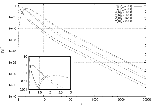
Figure 1: Plot of fermion functions $|\xi_{i}|^{2}$, where $\xi_{i}=\{\psi_{L},~{}\chi_{L}\}$ for the different values of the electrical charge in the background of nonextremal charged black string. The other parameters are equal to $m_{f}=2.7$, $N=1$, $m=1/2$, $q_{r}=5$, $\omega=k=0$.

In Fig.1 we plot $|\psi_{L}|^{2}$ and $|\chi_{L}|^{2}$ as a function of $r$-coordinate, for various values of the electric charge $q_{e}$. We set $q_{e}=0.0,~{}10.0,~{}50.0$ and ${m}_{fer}=2.7$, the winding number equals to $1$, the Higgs charge $q_{r}=5$ and $m=1/2,~{}\omega=0,~{}k=0$. We shall first consider the case of non-extremal charged black string.
The solution with $q_{e}=0$ is responsible for uncharged fermion field being the eigenstates of $\gamma^{0}\gamma^{3}$ matrices. The fermion functions $|\psi_{L}|^{2}$ and $|\chi_{L}|^{2}$ for the uncharged case are divergent near the black string event horizon. On the contrary, the fermion function describing the charged fermions are regular in the nearby of the aforementioned event horizon. The smaller $q_{e}$ we consider the closer the black string event horizon they begin to condensate.

Finally we note that at the beginning, when $q_{e}$ is small, fermions start to condensate just outside the black string event horizon but inside the cosmic string core. These fermions are trapped as massless modes inside the Abelian Higgs vortex and they can lead to superconductivity. On the contrary, for larger $q_{e}$, the electrostatic interactions among fermions and charge black string may eventually cause the expulsion of the fermions from the considered cosmic string and destroy superconductivity. One should mention that the electric charge has also a great influence on the width of the region where fermion function $|\xi_{i}|^{2}$ values are different from zero (let us say $|\xi_{i}|^{2}>10^{-10}$). Namely, the greater $q_{e}$ is the larger is the width in question.
For each electric charge, one can find a specific value $r_{e}$ of the $r$-coordinate (for $q_{e}=10,~{}r_{e}=1.3,~{}q_{e}=50,~{}r_{e}=2.8$), where one has that for $r>r_{e}$ the function $|\psi_{L}|^{2}$ has the greater values than $|\chi_{L}|^{2}$. On the other hand, when $r<r_{e}$, the behaviour of the functions in question reverses.

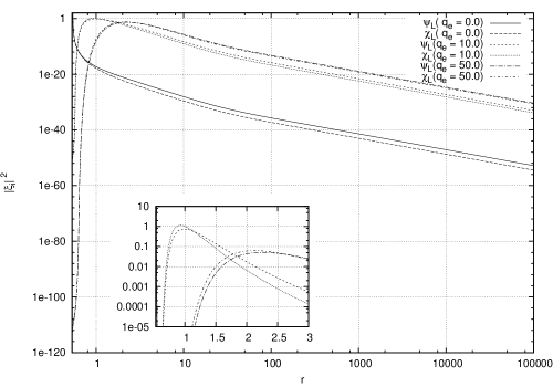
Figure 2: Plot of fermion functions $|\xi_{i}|^{2}$, where $\xi_{i}=\{\psi_{L},~{}\chi_{L}\}$ for the different values of the electrical charge in the background of extremal charged black string. The other parameters as in Fig.1.

In Fig.2 we have elaborated the dependence of the fermion functions $|\psi_{L}|^{2}$ and $|\chi_{L}|^{2}$ on the electric charge for the extremal charged black string. We took into account the same values of the electric charge and other parameters as in Fig.1. It turns out, that the uncharged fermion functions for which $q_{e}=0$ are divergent near the extremal black string event horizon. On the other hand, the charged fermion functions are regular in the vicinity of it. We also have the same dependence of the electric charge, i.e., the greater value of electric charge we have the farther from the event horizon of the extremal black string fermion fields begin to condensate. Comparing this effect in the spacetime of both types of black strings one remarks that the extreme black string far more expels fermion fields that the nonextremal one. There is also the specific value $r_{e}$ ($q_{e}=10,~{}r_{e}=1.15,~{}q_{e}=50,~{}r_{e}=2.7$), for which $r<r_{e}$ we acquire that $|\psi_{L}|^{2}<|\psi_{L}|^{2}$ and $r>r_{e}$ function $|\psi_{L}|^{2}$ has greater values than $|\chi_{L}|^{2}$.

In Fig.3 and Fig.4 we depicted the dependence of the fermion functions on the various values of the Higgs charge. Namely, we take into account $q_{r}=0.0,~{}5.0,~{}10.0$. The electric charge was put to the constant and equaled to $10.0$. The other parameters are the same as in Fig.1. Fig.3 is valid for the non-extremal charged black string, while Fig.4 is connected with the extremal case. The close inspection of the above figures reveals that $q_{r}$ has no influence on the regularity of the fermion solutions near the black string event horizon. For instance, for $q_{e}=10$ and $q_{r}=0$ the obtained solution is regular in the vicinity of the event horizon. However, the greater value of the Higgs charge one considers the closer to the black string event horizon fermions condensate. For given value of the electric charge one has that the greater value of the Higgs charge we take into account the smaller width of the region where $|\xi_{i}|^{2}$ is considerably different from zero and the larger maximal value of $|\xi_{i}|^{2}$ we obtain.

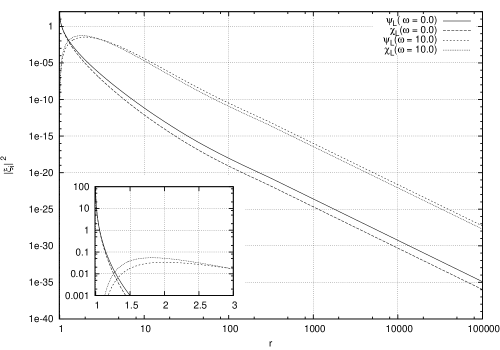
Figure 5: Dependence of fermion functions $|\xi_{i}|^{2}$, where $\xi_{i}=\{\psi_{L},~{}\chi_{L}\}$ on the different values of $\omega$. We set the winding number equal to $1$. The other parameters are are chosen to be $m_{f}=2.7$, $N=1$, $m=1/2$, $q_{r}=5$, $q_{e}=0$, $k=0$. The nonextremal charged black string and electrically charged spinors case.

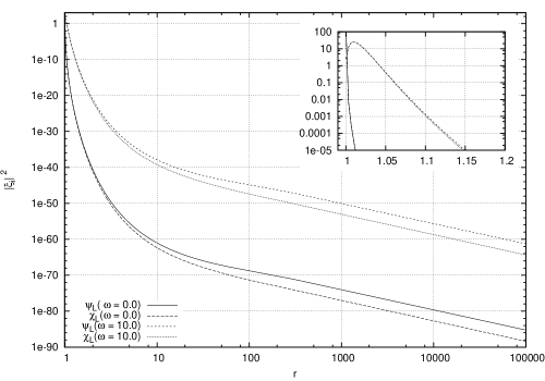
Figure 6: Dependence of fermion functions $|\xi_{i}|^{2}$, where $\xi_{i}=\{\psi_{L},~{}\chi_{L}\}$ on the different values of $\omega$. We put $N=10$. The other parameters are the same as in Fig.5. The nonextremal charged black string and electrically charged spinors case.

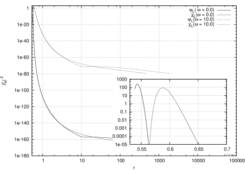
Figure 8: Dependence of fermion functions $|\xi_{i}|^{2}$ where $\xi_{i}=\{\psi_{L},~{}\chi_{L}\}$ on the different values of $\omega$ and the winding number $N=10$. The other parameters we set as in Fig.5. The extremal charged black string and electrically charged spinors case.

Now, we proceed to analyze the influence of the non-zero energy ($\omega\neq 0$) on the charged fermion functions. In Fig.5 we study the nonextremal black string. The parameters we choose as ${m}_{fer}=2.7$, the winding number $N=1$, $m=1/2$, the Higgs charge $q_{r}=5$ and $q_{e}=0,~{}k=0$. We set $\omega=0.0,~{}10.0$. As we can see, even in the uncharged case, for the large enough $\omega$ we get solution regular in the nearby of the event horizon. For $r>r_{e}=2.9$ one has that $|\psi_{L}|^{2}>|\chi_{L}|^{2}$, but for $r<r_{e}$ the dependence reverses. In Fig.6 the parameters are the same as in Fig.5 but we consider the larger value of the winding number $N=10$. Now, the larger value of the winding number caused that the localization of the fermion began closer to the black string event horizon. For $r>r_{e}=1.07$ one has that $|\psi_{L}|^{2}>|\chi_{L}|^{2}$, but when $r$ exceeds $r_{e}$ one arrives at the conclusion that $|\chi_{L}|^{2}>|\psi_{L}|^{2}$.
In Fig.7 and Fig.8 we take into account the same case of the non-zero modes for the extremal black string. Namely, in Fig.7 the parameters are the same as in Fig.5 and we arrive at the regular solution with $r_{e}=1.2$. For the case when $N=10$ one obtains that the curves depicting the behaviour of fermion functions intersect more than one time and the closer value of $r_{e}$ to the black string event horizon is equal to $1.55$. When we consider the larger value of winding number we achieve the closer to the event horizon localization of fermion functions in question. The other interesting feature is that for large N, even for $q_{e}=\omega=0$, we get regular solution in the vicinity of the event horizon.

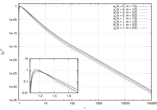
Figure 9: Fermion functions $|\xi_{i}|^{2}$, where $\xi_{i}=\{\psi_{L},~{}\chi_{L}\}$ for different values of $k$ and $m$ in the background of nonextremal charged black string. The other parameters are given by $m_{f}=2.7$, $N=1$, $q_{r}=5$, $q_{e}=10$, $\omega=0$.

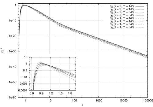
Figure 10: Fermion functions $|\xi_{i}|^{2}$, where $\xi_{i}=\{\psi_{L},~{}\chi_{L}\}$ for different values of $k$ and $m$ in the background of extremal charged black string. The rest of the parameters are set as in Fig.9.

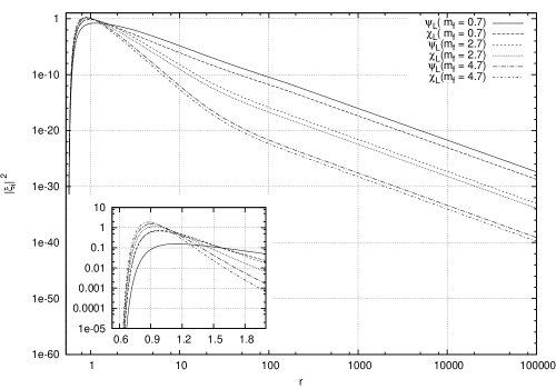
Figure 12: Dependence of fermion functions $|\xi_{i}|^{2}$, where $\xi_{i}=\{\psi_{L},~{}\chi_{L}\}$ on fermion mass for the extremal charged black string. The rest of the parameters are as in Fig.11.

In Fig.9 and Fig.10 we presented the behaviour of fermion functions for the different values of $k$ and $m$. The remaining parameters are the same as in the previous plots. One can conclude that near horizon of the extremal charged black string the fermion condensation takes place farther comparing to the nonextremal black string.
Fig.11 and Fig.12 are connected with the influence of the fermion mass ${m}_{fer}$ on the fermion functions in question. We set ${m}_{fer}=0.7,~{}~{}2.7,~{}4.7$ and the other parameters as in the previous cases. For each fermion mass, one attains that there is such a value $r_{e}$ for which one has that when $r>r_{e}$, then $|\psi_{L}|^{2}>|\chi_{L}|^{2}$ and for $r<r_{e}$ we get $|\psi_{L}|^{2}<|\chi_{L}|^{2}$. Moreover, the larger value of ${m}_{fer}$ is the smaller value of the fermion function one receives. Near the charged black string event horizon the situation in question changes. It turns out, that the bigger mass we have the larger value is achieved by fermion function. The tendency that the extremal charged black string expels fermions more violently is maintained.

VIII Conclusions

In our paper we have considered the problem of an Abelian Higgs vortex in the spacetime of a charged black string in the presence of Dirac fermion fields. Dirac fermions were coupled to the Abelian gauge fields $A_{\mu}$ and to the Abelian Higgs field $B_{\mu}$ as in the Witten’s model of the superconducting cosmic string wit85 . Moreover, we assume the complete separation of the degrees of freedom in the system in question. One has studied the extremal and nonextremal case of the black string pierced by an Abelian Higgs vortex. As far as the fermion function is concerned, we take into account the case of the uncharged, fermions being the eigenstates of $\gamma^{0}~{}\gamma^{3}$ gamma matrices, as well as the charged fermions. It was revealed that in the case of the uncharged fermions we obtained the divergent solutions near the charged black string event horizon both in extremal and nonextremal cases. On the contrary, the charged fermion functions are regular in the vicinity of the black string. The dependence of the fermion functions on the electric charge $q_{e}$ was elaborated. Namely, the smaller $q_{e}$ was, the closer to the event horizon fermions began to condensate. The same tendency was found in the case of the extremal charged black string. However, one remarks that the charged extremal black string expels fermion fields far more violently than the nonextremal one.

It worth mentioning that the Higgs charge also plays the dominant role on the behaviour of fermion functions in the nearby of the black string event horizon. Namely, when we put $q_{e}$ equal to a constant value, it turned out that the greater value of the Higgs charge we considered the closer to the event horizon fermion fields began to condensate. This was the case for both types of the black strings. Nevertheless, for the nonextremal charged black string the condensation took place far more closer to the event horizon than in the case of the extremal black string.

It is a remarkable fact that electric charge and Higgs charge are two parameters which have a great influence on the fermions in question. Especially, the fermion condensation depends on them. The increase of the electric charge provides the expulsion of fermions from the charged black string event horizon and eventually even from the cosmic string core. In turn, it can destroy superconductivity of the cosmic string in question, because of the lack of charge carriers inside the core. Consequently, for large enough electric charge, instead of a superconducting cosmic string, one has an onion-like structure. This structure consists of black string surrounded by cosmic string which in turn is encompassed by a shell of the fermionic condensate. Moreover, one has that for the larger value of the charge is taken into account the larger width of the aforementioned shell one achieves. By the width of the shell in question we understand the region where $|\xi_{i}|^{2}$ are different from zero, e.g., $|\xi_{i}|^{2}>10^{-10}$.
Returning to the consideration of the Higgs charge, one can remark that the situation is totally different. The increase of the Higgs charge implies the closer to the charged black string event horizon condensation of fermion fields and the decrease of the width of fermion condensate shell.

The winding number has also the influence on the behaviour of the considered fermion functions $|\psi_{L}|^{2}$ and $|\chi_{L}|^{2}$. For the established values of electric, Higgs charges, fermion mass, and for nonzero energy modes, one obtains that the greater $N$ is the closer to the event horizon fermions begins to concentrate. Fermion functions depend also on fermion mass $m_{fer}$. There is a point $r_{e}$ for which one has that, if $r>r_{e}$ then the smaller value of $m_{fer}$ one studies the the larger value of fermion function we attain. However, with the passage of $r$-coordinate in the direction to the event horizon, i.e., $r<r_{e}$, the situation alters.

By virtue of the revealed features of the fermion functions in the background of a charged black string pierced by an Abelian Higgs vortex, one can draw a conclusion that in principle there is such a value of the electric charge which can destroy fermionic superconductivity. The winding number and Higgs charge also exert a great influence on the superconductivity carried by an Abelian Higgs vortex penetrating the black string in question. This is the case for both extremal and nonextremal charged black string vortex systems.

Figure 3: Plot of fermion functions $|\xi_{i}|^{2}$, where $\xi_{i}=\{\psi_{L},~{}\chi_{L}\}$ for the different values of the Higgs charge in the background of nonextremal charged black hole. The other parameters we set $m_{f}=2.7$, $N=1$, $m=1/2$, $q_{e}=10$, $\omega=k=0$.

Figure 4: Plot of fermion functions $|\xi_{i}|^{2}$, where $\xi_{i}=\{\psi_{L},~{}\chi_{L}\}$ for the different values of the Higgs charge. The charged extremal black string case. The other parameters as in Fig.3.

Figure 7: Dependence of fermion functions $|\xi_{i}|^{2}$, where $\xi_{i}=\{\psi_{L},~{}\chi_{L}\}$ on the different values of $\omega$. We choose the winding number $N=1$. The other parameters are the same as in Fig.5. The extremal charged black string and electrically charged spinors case.

Figure 11: Dependence of fermion functions $|\xi_{i}|^{2}$, where $\xi_{i}=\{\psi_{L},~{}\chi_{L}\}$ on fermion mass for the nonextremal charged black string. The values of the parameters are: $N=1$, $q_{r}=5$, $q_{e}=10$, $\omega=k=0$.

References

- (1)
-
(2)
J.P.Lemos, Class. Quantum Grav. 12 , 1081 (1995),
J.P.Lemos, Phys. Lett. B 353, 46 (1995). - (3) J.P.Lemos and V.T.Zanchin, Phys. Rev. D 54, 3840 (1996).
- (4) M.H.Dehghani and N.Farhangkhah, Phys. Rev. D 71, 044008 (2005).
- (5) M.H.Dehghani, Phys. Rev. D 66, 044006 (2002).
- (6) M.H.Dehghani and T.Jalali, Phys. Rev. D 66, 124014 (2002).
- (7) A.Vilenkin and E.P.S.Shallard, Cosmic Strings and Other Topological Defects, Cambridge University Press, Cambridge (1994).
- (8) M.Aryal, L.H.Ford, and A.Vilenkin, Phys. Rev. D 34, 2263 (1986).
- (9) A.Achucarro, R.Gregory, and K.Kuijken, Phys. Rev. D 52, 5729 (1995).
-
(10)
A.Chamblin, J.M.A.Ashbourn-Chamblin, R.Emparan, and A.Sorborger, Phys. Rev. D 58, 124014 (1998),
A.Chamblin, J.M.A.Ashbourn-Chamblin, R.Emparan, and A.Sorborger, Phys. Rev. Lett. 80, 4378 (1998). -
(11)
F.Bonjour and R.Gregory, Phys. Rev. Lett. 81, 5034 (1998),
F.Bonjour, R.Emparan, and R.Gregory, Phys. Rev. D 59, 084022 (1999). -
(12)
M.Rogatko, Phys. Rev. D 64, 064014 (2001),
R.Moderski and M.Rogatko, ibid. 67, 024006 (2003),
M.Rogatko, ibid. 69, 044022 (2004),
R.Moderski and M.Rogatko, ibid. 69, 084018 (2004),
R.Moderski and M.Rogatko, ibid. 74, 044002 (2006). -
(13)
A.K.M.Massod-ul-Alam, Class. Quantum Grav. 10, 2649 (1993),
M.Mars and W.Simon, Adv. Theor. Math. Phys. 6, 279 (2003),
M.Rogatko, Class. Quantum Grav. 14, 2425 (1997),
M.Rogatko, Phys. Rev. D 58, 044011 (1998),
M.Rogatko, ibid. 59, 104010 (1999),
M.Rogatko, ibid. 82, 044017 (2010),
M.Rogatko, Class. Quantum Grav. 19, 875 (2002). - (14) R.Moderski and M.Rogatko, Phys. Rev. D 57, 3449 (1998).
- (15) R.Moderski and M.Rogatko, Phys. Rev. D 58, 124016 (1998).
- (16) R.Moderski and M.Rogatko, Phys. Rev. D 60, 104040 (1999).
- (17) S.Chandrasekhar, The Mathematical Theory of Black Holes, Oxford University Press, Oxford (1992).
- (18) G.W.Gibbons and A.R.Steif, Phys. Lett. B 314, 13 (1993).
- (19) I.Sakalli and M.Halilsoy, Phys. Rev. D 69, 124012 (2004).
- (20) D.Lohiya, Phys. Rev. D 30, 1194 (1984).
- (21) F.Finster, J.Smoller, and S.T.Yau, Adv. Theor. Math. Phys. 4, 1231 (2000).
-
(22)
F.Finster, J.Smoller, and S.T.Yau, Nucl. Phys. B 584, 387 (2000),
F.Finster, J.Smoller, and S.T.Yau, Mich. Math. j. 47, 199 (2000),
F.Finster, J.Smoller, and S.T.Yau, Commun. Math. Phys. 205, 249 (1999),
F.Finster, J.Smoller, and S.T.Yau, J. Math. Phys. 41, 2173 (2000). - (23) G.Silva-Ortigoza, Gen. Rel. Grav. 33, 395 (2001).
- (24) I.Sakalli, Gen. Rel. Grav. 35, 1321 (2003).
- (25) G.W.Gibbons and A.R.Steif, Phys. Lett. B 320, 245 (1994).
- (26) J.L.Jing, Phys. Rev. D 70, 065004 (2004).
- (27) J.L.Jing, Phys. Rev. D 72, 027501 (2005).
- (28) L.M.Burko and G.Khanna, Phys. Rev. D 70, 044018 (2004).
- (29) X.He and J.L.Jing, Nucl. Phys. B 755, 313 (2006).
- (30) G.W.Gibbons and M.Rogatko, Phys. Rev. D 77, 044034 (2008).
- (31) M.Góźdź, L.Nakonieczny, and M.Rogatko, Phys. Rev. D 81, 104027 (2010).
- (32) M.Góźdź and M.Rogatko, Int. J. Mod. Phys. E 20, 507 (2011).
-
(33)
G.W.Gibbons, M.Rogatko, and A.Szyplowska, Phys. Rev. D 77, 064024 (2008),
M.Rogatko and A.Szyplowska, Phys. Rev. D 79, 104005 (2009). - (34) K.S.Cheng, Y.W.Yu, and T.Harko, Phys. Rev. Lett. 104, 241102 (2010).
- (35) N.Nagano and A.A.Watson, Rev. Mod. Phys 72, 689 (2000).
- (36) R.Gregory and J.A.Harvey, Phys. Rev. D 46, 3302 (1992).
- (37) E.Witten, Nucl. Phys. B 249, 557 (1985).
- (38) L.Nakonieczny and M.Rogatko, Phys. Rev. D 84, 044029 (2011).
- (39) Y.Brihaye and B.Hartmann, JHEP 09, 002 (2010).
- (40) Y.Brihaye and B.Hartmann, Phys. Rev. D 83, 126008 (2011).
- (41) R.Jackiw and P.Rossi, Nucl. Phys. B 190, 681 (1981).
- (42) P. Hartman, Ordinary differential equations. Second edition , SIAM 2002
- (43) M.H.Dehghani, A.M.Ghezelbash, and R.B.Mann, Nucl. Phys. B 625, 389 (2002).
- (44) W. H. Press, S. A. Teukolsky, W. T. Vetterling, and B. P. Flannery, Numerical Recipes in C, Cambridge University Press, Cambridge (1992).