Long-term X-ray variability of Swift J1644$+$57

Abstract

We studied the X-ray timing and spectral variability of the X-ray source Sw J1644$+$57, a candidate for a tidal disruption event. We have separated the long-term trend (an initial decline followed by a plateau) from the short-term dips in the Swift light-curve. Power spectra and Lomb-Scargle periodograms hint at possible periodic modulation. By using structure function analysis, we have shown that the dips were not random but occurred preferentially at time intervals $\approx(2.3,4.5,9)\times 10^{5}$ s and their higher-order multiples. After the plateau epoch, dipping resumed at $\approx(0.7,1.4)\times 10^{6}$ s and their multiples. We have also found that the X-ray spectrum became much softer during each of the early dip, while the spectrum outside the dips became mildly harder in its long-term evolution. We propose that the jet in the system undergoes precession and nutation, which causes the collimated core of the jet briefly to go out of our line of sight. The combined effects of precession and nutation provide a natural explanation for the peculiar patterns of the dips. We interpret the slow hardening of the baseline flux as a transition from an extended, optically thin emission region to a compact, more opaque emission core at the base of the jet.

1 Introduction

Swift J164449.3$+$573451 (henceforth, Sw J1644$+$57) was discovered by the Swift Burst Alert Telescope (BAT; Gehrels et al., 2004; Barthelmy et al., 2005) on 2011 March 28 (Cummings et al., 2011; Burrows et al., 2011). The long duration of the X-ray emission and flaring events (still ongoing after 8 months), and the spatial coincidence with the nucleus of a galaxy at redshift $z=0.354$ (luminosity distance $\approx 5.7\times 10^{27}$cm: Levan et al., 2011b, a; Thoene et al., 2011) made it clear that it was not a Gamma-Ray-Burst, and was instead associated to some kind of sudden accretion event onto a supermassive black hole (BH) (Bloom et al., 2011b; Burrows et al., 2011; Levan et al., 2011a). In particular, the precise position from Very Large Array and Very Long Baseline Array radio observations clinched the identification of the X-ray source with the nucleus of the host galaxy (Zauderer et al., 2011). The lack of previous evidence of nuclear activity (AGN) from the same source, and the short timescale for the outburst rise (a few days: Krimm & Barthelmy, 2011) are difficult to reconcile with changes in the large-scale accretion flow through an accretion disc, but this scenario is not completely ruled out (Burrows et al., 2011). The most favoured scenario is a tidal disruption event deep inside the sphere of influence of the BH (Bloom et al., 2011a, b; Burrows et al., 2011; Cannizzo, Troja & Lodato, 2011; Socrates, 2011). The nature of the star being disrupted (and therefore the radius at which the event occurs and the timescale on which the stellar material circularised into a disc and accreted) are still matters of intense debate. For example, it was argued that if the disrupted star were a white dwarf, the smaller tidal disruption radius and characteristic timescale would be more consistent with the observed duration of the flares (Krolik & Piran, 2011).

There are no direct measurements of the BH mass ($M_{\bullet}$). Indirect order-of-magnitude constraints consist of: an upper limit to the BH mass that permits tidal disruption events outside the event horizons (Rees, 1988); a minimum variability timescale $\sim 100$ s that sets an upper limit to the light-crossing timescale (Bloom et al., 2011b; Burrows et al., 2011); and well known empirical relations between $M_{\bullet}$ and the host galaxian environment (whatever causes those trends, e.g. Silk & Rees, 1998; Jahnke & Macciò, 2011). For example, based on the optical luminosity of the host galaxy, Levan et al. (2011a) estimate a spheroidal stellar mass $M_{\rm sph}\sim 10^{9}$–$10^{10}M_{\odot}$. Using the log-linear spheroidal mass–BH mass relation of Bennert et al. (2011) (see also Magorrian et al. 1998; Lauer et al. 2007; Kormendy, Bender & Cornell 2011), this implies a likely BH mass $2\times 10^{6}M_{\odot}\la M_{\rm BH}\la 10^{7}M_{\odot}$ (Levan et al., 2011a); adopting instead the bent $M_{\rm sph}$–$M_{\rm BH}$ relation of Graham (2012), it allows also a lower range of BH masses, $10^{5}M_{\odot}\la M_{\rm BH}\la 10^{7}M_{\odot}$. The latter range is more consistent with the BH mass $\log(M_{\bullet}/M_{\odot})=5.5\pm 1.1$ estimated by Miller & Gültekin (2011), based on empirical “fundamental plane” relations between radio and X-ray luminosities of accreting BHs.

The relatively small BH mass implies a bolometric Eddington luminosity $\la 10^{45}$ erg s^-1, and a $0.3$–$10$ keV luminosity a few times smaller. The average isotropic luminosity in the $0.3$–$10$ keV band was $\approx 10^{47}$ erg s^-1 in the first few weeks after the initial outburst; several months ($\sim 10^{7}$ s) later, it was still $\approx$ a few $\times 10^{45}$ erg s^-1, well above the Eddington limit. This is strong evidence that the emission is beamed towards us (Bloom et al., 2011b; Burrows et al., 2011; Levan et al., 2011a), and is probably associated with a relativistic jet, like in blazars. A relativistic jet has also been invoked to explain the radio transient event, interpreted as an external shock in the gas surrounding Sw J1644$+$57 (Bower, Bloom & Cenko, 2011; Zauderer et al., 2011; Burrows et al., 2011). The Lorentz factor of the jet is highly uncertain, with estimates varying from $\Gamma\approx 2$–$5$ (Zauderer et al., 2011) to $\Gamma\approx 10$–$20$ (Bloom et al., 2011b; Burrows et al., 2011). The rarity of the event, with one such outburst discovered in 7 years of Swift operations, is consistent with the theoretical expectations of tidal disruption rates and jet opening angle $\theta\sim 5^{\circ}$, corresponding to $\Gamma\approx 1/\theta\approx 10$.

The origin of the photon emission is still unclear. There are clearly at least two prominent peaks in the spectral energy distribution: one in the far IR and one in the hard X-ray band (Bloom et al., 2011b; Burrows et al., 2011). They can be modelled as direct synchrotron emission (single-component model) from radio to X-rays, with strong dust extinction in the optical/UV band. Alternatively, the radio/IR peak is the direct synchrotron emission and the X-ray peak is due to inverse Compton scattering of external photons, most likely disc photons (two-component blazar model). A third possibility is that the X-ray emission is due to inverse Compton emission at the base of the jet, while the radio/IR synchrotron emission comes from the forward shock at the interface between the head of the jet and the interstellar medium (Bloom et al., 2011b).

The X-ray spectrum is well fitted by a simple absorbed power-law, although more complex models were also discussed (Burrows et al., 2011). The average photon index during the first $\approx 2\times 10^{5}$ s is $\Gamma\approx 1.8$ (Levan et al., 2011a; Burrows et al., 2011). However, the physical meaning of this average value has to be interpreted more carefully, as there are strong variations in hardness and photon index between flares, with $\Gamma$ changing between $\approx 1.3$ and $3$ (Levan et al., 2011a). In particular, the photon index is harder when the source is brighter (Kennea et al., 2011; Bloom et al., 2011a; Levan et al., 2011a; Burrows et al., 2011).

In the Swift X-Ray Telescope (XRT; Burrows et al., 2005) band, $0.3$–$10$ keV, the decline in flux was initially consistent with the $t^{-5/3}$ decay (Levan et al., 2011a; Bloom et al., 2011b) expected for the spreading and accretion of fallback material after a tidal disruption event. Bloom et al. (2011b) used the early Swift/XRT observations (up to $t\approx 4.5\times 10^{6}$ s) to study the power spectral density over the $0.1$–$100$ mHz frequency range: they found no significant feature that is not associated with the orbital period of the spacecraft. By contrast, a series of XMM-Newton Target-of-Opportunity observations during the initial decline phase suggested the presence of a 4.7-mHz ($\approx 200$ s) quasi periodic oscillation (Miller & Strohmayer, 2011), and showed short-term variability over the $0.4$–$100$ mHz range. If the putative quasi-periodic oscillation corresponds to the Keplerian frequency at the innermost stable circular orbit of a Schwarzschild BH, it would imply a BH mass $\sim 5\times 10^{5}M_{\odot}$ (Miller & Strohmayer, 2011).

Possible variability on the $\sim 10^{-7}$–$10^{-4}$ Hz frequency range has not been investigated in much detail yet. The ongoing series of Swift/XRT monitoring observations, which have now followed the source for $\approx 2\times 10^{7}$ s, offer the best chance for this study. Luckily, eight months after the outburst, the source is still detected at a flux $\approx 10^{-11}$ erg cm^-2 s^-1 in the $0.3$–$10$ keV band, declining only very slowly. In this paper, we examine the X-ray variability over the $10^{4}$–$10^{7}$ s timescale, looking for phenomenological patterns (characteristic variability timescales, spectral evolution) that can help us test physical scenarios. In particular, we want to determine whether the dips that characterise the X-ray light-curve are random or have some periodicity, and we discuss the X-ray changes during the dips.

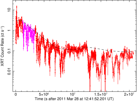
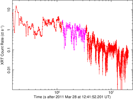
Figure 1: Top panel: Swift/XRT $0.3$–$10$ keV light-curve between 2011 March 28 and 2011 November 28, plotted on a linear time scale. Datapoints in red are taken in PC mode; those in magenta are in WT mode. The dashed curve is a phenomenological function used to de-trend the data and “normalise” the continuum. Bottom panel: same as in the top panel, but on a logarithmic time scale.

2 Data analysis

Sw J1644$+$57 has been monitored by the XRT several times a day, every day since 2011 March 28. We used the on-line Swift/XRT data product generator (Evans et al., 2007, 2009) to extract light-curves in different energy bands, and spectra (including background and ancillary response files) in different time intervals; we selected grade 0–12 events. We downloaded the suitable spectral response files for single and double events in photon-counting (PC) mode and window-timing (WT) mode from the latest Calibration Database. We used XSPEC Version 12 (Arnaud, 1996) for spectral analysis, and standard FTOOLS (Blackburn, 1995) tasks for preliminary timing analysis — for example, for defining the time intervals that were used to extract intensity-selected spectra. For more advanced timing analyses, we used a Lomb-Scargle periodogram and structure function analysis, (discussed in Section 3).

A caveat for timing analysis is that the observational data are irregularly sampled; the duration of each snapshot observation in either WT or PC mode (typically, a few hundred seconds) and the temporal gaps between observations are not constant. Irregular, gappy data sequences are accommodated within the formulation of LS-periodograms (§ 3.2.2), where data are at discrete events rather than long temporal bins. Such imperfections however are unnatural to conventional Fourier (§ 3.2.1) and structure function methods (§ 3.2.3). There are various strategies that can circumvent this issue: we considered the hyphen method, the zigzag method and the trapezoid method. In the hyphen method the gaps are practically omitted. The flux levels are set to be locally constant for the durations of the data bins. In the zigzag method, a data point is set at the mid-time of each observational bin, and we connect each point linearly to the next consecutive data point. The numerical light curve is piecewise linear and resembles a polygonal landscape. In a variant trapezoid method, the observational bins are treated as piecewise flat segments as in the hyphen method but the gaps are connected directly with diagonal lines.

As the covering factor of the bins is small in the hyphen method, unless the data are numerically bridged, we found that the calculated power spectra and structure functions tend to blur any useful information in the noise. Instead, we found that the zigzag method tends to provide robust results for power spectra and structure functions. The results obtained with the trapezoid method are indistinguishable from those of the zigzag method. Thus, we present here only the results from analyses done with the zigzag method.

3 Main results

3.1 Different phases in the lightcurve

Figure 1 shows the XRT $0.3$–$10$ keV light-curve, binned by snapshot (typical exposure duration $\sim$ a few 100 s). The luminosity evolution shows a series of phases with different phenomenological properties. During the first three months after the outburst — in particular, at times $2\times 10^{5}~{}{\rm s}\la t\la 9\times 10^{6}$ s — the baseline trend is adequately fitted by an exponential decay, with an e-folding timescale of $\approx 2.0\times 10^{6}$ s. Flares and complex dips are superposed onto this trend. In other work (Levan et al., 2011a), a more canonical tidal-disruption decline scaling $\sim t^{-5/3}$ was fitted to the same section of the light-curve; the difference is mostly due to a different definition of the baseline. Later we will show a change in the variability at $t\approx 4.7\times 10^{6}$ s, which distinguishes “early” and “late” epochs of the declining stage. For $t\ga 9\times 10^{6}$ s, the decay stopped and the source appeared to settle on a “plateau” (XRT count rate $\approx 0.1$ ct s^-1), without any dips. Broader dips resumed for $t\ga 12.5\times 10^{6}$ s (the “recent” epoch), but the baseline level has not significantly declined below $\approx 0.1$ ct s^-1.

Because of the different behaviour of the light-curve at different epochs, we shall investigate the short-term variability separately in the different phases. We also note that the state transitions are each a continuous, gradual evolution of flux, timing and spectral properties over time. Therefore the choice of start and end times defining the different epoch sub-intervals are somewhat arbitrary (to within a few $10^{5}$ s) and do not affect the main conclusions of our study.

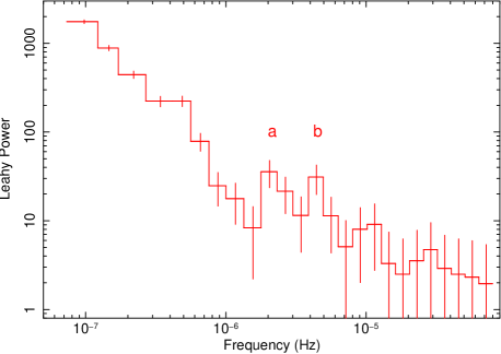
Figure 2: Power spectrum of the Swift/XRT light curve (combining data in WT and PC mode), excluding the first $2\times 10^{5}$ s. The input data have been binned to 5000 s intervals. The power spectrum is normalised (Leahy et al., 1983) such that its integral gives the squared rms fractional variability (i.e., the Y axis is in units of (rms)² Hz^-1), and the expected white noise level $\approx 2$. Two features at $\mu$Hz frequencies (labelled in the plot) are suggestive of periodicities on timescales $\approx(2.3\pm 0.3)\times 10^{5}$ s and about twice that value.

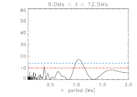
Figure 3: Lomb-Scargle periodograms of the light-curve in four time intervals of interest. The data have not been de-trended. In the first, second and fourth of these intervals, there are plausible periodicities: significant at the 1% FAP level (with two definitions of this threshold marked as horizontal lines).

3.2 Search for periodicities

3.2.1 Fourier analysis

Fourier techniques, as implemented for example in the XRONOS powspec timing analysis task (Stella & Angelini, 1992), are widely used for the timing analysis of X-ray lightcurves in AGN and X-ray binaries. The standard technique of dividing the lightcurve into multiple intervals, calculating the power density spectrum in each interval, and taking the mean of the power density values (and corresponding standard deviations) is applicable only if the process is ergodic (Priestley, 1988; Guidorzi, 2011), so that time averages can be substituted for ensemble averages. In the case of highly non-stationary events like Sw J1644$+$57, Gamma-ray bursts, or X-ray flares, it does not make sense to subdivide the light-curve into sub-intervals, and the power density spectrum has to be calculated over the entire duration of the observation (Guidorzi, 2011). We did that, and then calculated the standard deviation for the power density at each frequency bin with the procedure outlined in Guidorzi (2011).

Figure 2 shows the power spectrum of the $0.3$–$10$ keV light-curve, excluding the first $2\times 10^{5}$ s (that is, after the huge initial flares have subsided). The root-mean-square (rms) power rises at lower frequencies, as $\sim\nu^{-1}$. This is mostly due to the long-term dimming trend. There appear to be two unresolved features at frequencies $\approx 2.2\mu$Hz and $4.5\mu$Hz; however, their power is comparable to the statistical uncertainty. This prevents us from firmly concluding whether there are true underlying periodicities or whether those features were just statistical noise. Moreover, Fourier analysis techniques are better suited to time series that are equispaced and with no time gaps. Neither condition is true in our case. The complex shape of the window and sampling functions may introduce side lobes (spectral leakage) in the discrete Fourier transform. In summary, we consider the features observed in the power density spectrum as suggestive of possible periodic signals, but not yet statistically significant, because of the shortcomings of the Fourier technique.

3.2.2 Lomb-Scargle periodogram

As an improvement over Fourier power spectrum analyses, Lomb (1976) and Scargle (1982) introduced a periodogram technique that proves to be more robust in the detection of periodicities in irregularly sampled light curves. Press & Rybicki (1989) accelerated the method, with a numerical modification based on fast Fourier transforms. The Lomb-Scargle periodogram is equivalent to a best-fit analysis of the data with a single sinusoidal function. The phase and amplitude emerge directly for the implied fit. The technique is observationally applied to diverse subjects: exoplanet detections; solar eruptions; variable and pulsating stars; high-energy accreting systems; ultracompact binaries (e.g. Desidera et al., 2011; Farrell et al., 2010; Foullon, Verwichte & Nakariakov, 2009; Hakala et al., 2003; Nataf, Stanek & Bakos, 2010; Ness et al., 2011; Omiya et al., 2011; Qian, Solomon & Mlynczak, 2010; Sarty et al., 2009; Uthas et al., 2012; Xu et al., 2011; Wen et al., 2006).

Figure 3 presents Lomb-Scargle plots of four stages of the light-curve: during the early decline ($4\times 10^{5}<t<4.7\times 10^{6}$ s), late decline ($4.7\times 10^{6}<t<9\times 10^{6}$ s), the plateau ($9\times 10^{6}<t<1.25\times 10^{7}$ s), and the recent post-plateau stage ($t>1.25\times 10^{7}$ s). We used a freely available IDL code implementing the formulation of Press & Rybicki (1989) and Horne & Baliunas (1986). Power and detection thresholds assume a grid of 1000 evenly spaced frequencies. For the sake of smoother curves, the curve is drawn with $10^{4}$ intermediate frequencies (not involved in the calculation of detection thresholds). In our plots, peak detection thresholds are marked in blue and red. Higher peaks are statistically significant at the 1% level (“false alert probability” FAP$=0.01$). The blue (dashed) threshold is $z_{0}$ in equation (18) of section III(c) of Scargle (1982). The red (dot-dashed) line is the threshold obtained from $10^{4}$ “white noise simulations” conservatively taking the light-curve’s total variance. The data are not de-trended, so the variance is an overestimate. The uncorrected decay timescale ($t_{0}\approx 2\times 10^{6}$ s) during the early and later decline ($t<9\times 10^{6}$ s) is probably responsible for artefacts at the long-period end of the periodograms (top panels of Figure 3).

At early times ($t<4.7\times 10^{6}$ s) there are peaks of varied significance at periods of $\tau\approx 0.23$, $0.45$, $0.9$ and $1.4$ Ms. The first two in this series correspond to the two features tentatively identified in the Fourier spectrum (§ 3.2.1). A characteristic spacing $\approx 0.45$Ms between dips is also inferred from a visual inspection of the early part of the XRT lightcurve (Figure 4). During later weeks of the decline ($4.7\times 10^{6}<t<9\times 10^{6}$ s) there is a stronger peak at period $\tau\approx 0.9$Ms. Later, during the plateau stage ($9\times 10^{6}\la t\la 12.5\times 10^{6}$ s), the power of the peaks is relatively low, consistent with the visible steadiness of the light-curve. There may be a feature at $\tau\approx 1.1\times 10^{6}$ s, which is near the 1% significance level, and perhaps another, weaker, feature at $\approx 0.4\times 10^{6}$ s. In the very latest times after the plateau, when dipping resumed ($t\ga 12.5\times 10^{6}$ s), there is a strong peak at $\tau\approx 1.4$Ms. This is consistent with a visual inspection of the last section of the lightcurve, as it is the characteristic spacing between major quasi-sinusoidal dips (Figure 4).

In summary, the Lomb-Scargle analysis gives signs of periodicity (which are stronger in some intervals than others), and these indications are clearer than from the Fourier analysis. We note that the Lomb-Scargle periodogram is by construction most sensitive to oscillations similar to a sine wave. Repetitive patterns that are highly non-sinusoidal may have their true significance understated. The dips seen in the early phases of the XRT lightcurve (Figure 4) are sharp and brief compared to the non-dip conditions: this is clearly far from a sinusoidal pattern. This motivates further study with another, broader technique.

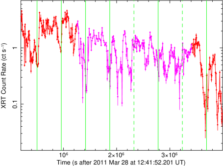
Figure 4: Top panel: zoomed-in view of an early section of the light-curve, showing a structure of recurrent dips, many of them consistent with a quasi periodic timescale of $\approx 4.5\times 10^{5}$ s (solid green lines). This kind of dip structure produces the characteristic frequency signal detected in the Lomb-Scargle periodograms and structure function analyses. However, some expected dips are skipped or premature (dashed green lines). Bottom panel: zoomed-in view of the last section of the light-curve observed to-date; the dips occur on a longer timescale.

$\begin{array}[]{llll}\hline\cr\\ \lx@intercol\hfil\tau/\tau_{0}\hfil\lx@intercol\\[5.0pt] \Delta t_{1},1\sigma&\Delta t_{1},3\sigma&\Delta t_{2},1\sigma&\Delta t_{2},3\sigma\\[5.0pt] \hline\cr\\ 0.514_{-0.038}^{+0.014}&0.514_{-0.074}^{+0.031}&0.478_{-0.037}^{+0.017}&0.478_{-0.059}^{+0.036}\\[5.0pt] 1.037_{-0.014}^{+0.024}&1.037_{-0.035}^{+0.043}&1.060_{-0.027}^{+0.017}&1.060_{-0.053}^{+0.040}\\[5.0pt] 1.555_{-0.026}^{+0.016}&1.555_{-0.046}^{+0.031}&1.501_{-0.020}^{+0.024}&1.501_{-0.034}^{+0.059}\\[5.0pt] 2.034_{-0.036}^{+0.020}&2.034_{-0.058}^{+0.036}&1.994_{-0.020}^{+0.031}&1.994_{-0.038}^{+0.053}\\[5.0pt] 2.455_{-0.024}^{+0.034}&2.455_{-0.051}^{+0.076}&2.464_{-0.034}^{+0.061}&2.464_{-0.056}^{+0.082}\\[5.0pt] 3.052_{-0.052}^{+0.033}&3.052_{-0.095}^{+0.057}&3.048_{-0.038}^{+0.048}&3.048_{-0.088}^{+0.076}\\[5.0pt] 3.558_{-0.027}^{+0.032}&3.558_{-0.048}^{+0.062}&3.585_{-0.052}^{+0.025}&3.585_{-0.092}^{+0.053}\\[5.0pt] 4.002_{-0.032}^{+0.045}&4.002_{-0.070}^{+0.084}&4.024_{-0.045}^{+0.025}&4.024_{-0.103}^{+0.065}\\[5.0pt] 4.498_{-0.044}^{+0.048}&&4.464_{-0.058}^{+0.058}&4.464_{-0.152}^{+0.089}\\[5.0pt] 5.066_{-0.190}^{+0.064}&5.066_{-0.245}^{+0.130}&4.976_{-0.027}^{+0.057}&4.976_{-0.097}^{+0.178}\\[5.0pt] 5.536_{-0.138}^{+0.035}&\\[5.0pt] 6.036_{-0.051}^{+0.074}&&6.139_{-0.112}^{+0.068}&6.139_{-0.173}^{+0.122}\\[5.0pt] &&7.629_{-0.139}^{+0.068}\\[5.0pt] 8.531_{-0.100}^{+0.108}&\\[5.0pt] \\ \hline\cr\end{array}$

Table 1: Timescale of regular features detected in the $S_{2}$ structure function for data extracted in the intervals $\Delta t_{1}=[0.4,8.9]\times 10^{6}$ s and $\Delta t_{2}=[1.0,8.9]\times 10^{6}$ s. Minima are tabulated if their depths exceed $1\sigma$ and $3\sigma$ locally, and are not enclosed within the catchment of another local minimum. To emphasise the periodicity, we express the timescales $\tau$ as multiples of a characteristic $\tau_{0}=0.445\times 10^{6}$ s.

3.2.3 Structure function technique

To obtain a more robust test of the presence or absence of periodicity in the X-ray luminosity variations, we carried out a more effective alternative analysis based on Kolmogorov’s structure functions (Kolmogorov, 1941, 1991). They are the statistical moments of a temporally varying signal, with the light curve compared to itself at an offset $\tau$. The $n^{\rm th}$-order structure function is

$$S_{n}(\tau)\equiv\langle{\left[{z(t+\tau)-z(t)}\right]^{n}}\rangle\ .$$ (1)

The second order structure function, $S_{2}$, is particularly useful for the purpose of time series analysis, as it describes the variance of a signal on timescales $\tau$. In addition to their original applications in the physics of turbulence (Brandenburg & Nordlund, 2011, and references therein), structure functions have a venerable history in the diagnosis of variability in blazars, other configurations of AGN, and various compact systems (e.g. Simonetti, Cordes & Heeschen, 1985; Cordes & Downs, 1985; Bregman et al., 1988; Hughes, Aller & Aller, 1992; Brinkmann et al., 2000, 2001; Kataoka et al., 2001; Iyomoto & Makishima, 2001; Tanihata et al., 2003; Wilhite et al., 2008; Emmanoulopoulos, McHardy & Uttley, 2010; Yusef-Zadeh et al., 2011; Voevodkin, 2011). In these contexts they are most often used to search for break frequencies that are supposed to characterise internal scales of the system, though Emmanoulopoulos, McHardy & Uttley (2010) warn users to beware of potential artefacts from sparsely sampled data. (Our data are densely sampled, even during the dips, and we are seeking signs of repetition rather than break scales.) Structure functions are also used to diagnose simulations of turbulence in interstellar media (Boldyrev, Nordlund & Padoan, 2002; Kritsuk et al., 2007, 2009; Schmidt, Federrath & Klessen, 2008), and synthetic observables of simulated jets and AGN (Saxton et al., 2002, 2010). In the Appendix, we show the procedures by which we compute the structure functions of various orders from data sets with unevenly sampled data. We also show how the corresponding uncertainties are determined. In the rest of this section, we report our main findings.

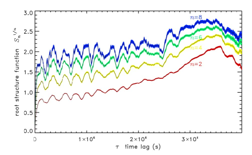
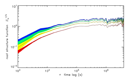
Figure 5: Structure functions of the Swift/XRT count rate at order $n=2,4,6,8$ (red, yellow, green and blue curves, respectively) for the light-curve interval $4\times 10^{5}{\rm s}<t<4.7\times 10^{6}$ s. The thickness of each curve indicates $1\sigma$ uncertainties. Top panel: result based on the direct XRT count rate, without correcting for the long-term decline. We interpret the rising trend towards the longest timescales ($\tau\ga 10^{6}$ s) as an artefact arising from the long-term dimming in the X-ray luminosity. Middle panel: result when the count rate is de-trended. Locally there is an $e$-folding timescale of $2\times 10^{6}$ s. Bottom panel: same as the middle panel, but plotted in logarithmic scale, to highlight the essentially featureless “red noise” at variability timescales $\tau\la 10^{5}$ s. For $\tau\la 10^{5}$ s, but longer than the orbital period of Swift ($\approx 5800$ s), the structure functions show a featureless power-law form $S_{n}\propto\tau^{n/2}$, indicating stochastic red noise.

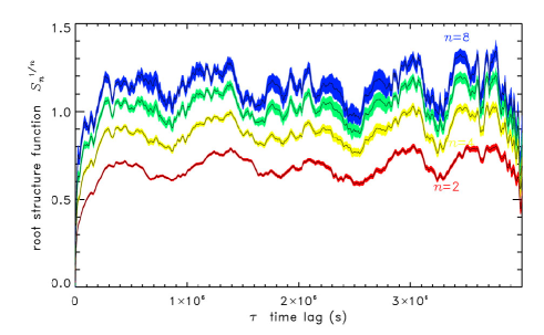
Figure 6: Top panel: structure functions of the de-trended X-ray count rate at order $n=2,4,6,8$ (red, yellow, green and blue curves, respectively) during the time interval $4.7\times 10^{6}{\rm s}<t<9.0\times 10^{6}$ s. A period at $\tau\approx 9\times 10^{5}$ s (and its multiples) is the dominant feature. The shorter periods that dominated earlier stages of the light-curve (Figure 5) are only slightly visible now, and only in higher-order structure functions. Bottom panel: structure functions in logarithmic scale, showing the white and red noise at small values of $\tau$.

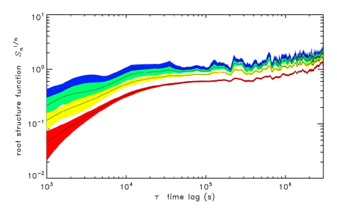
Figure 7: As in Figure 6, for $9.0\times 10^{6}{\rm s}<t<12.5\times 10^{6}$ s.

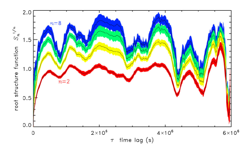
Figure 8: Structure functions of the detrended X-ray light-curve, for the recent epoch following the end of the plateau stage. The top panel is integrated over the whole available sequence, ($t>1.25\times 10^{7}$ s). The bottom panel uses only a shorter interval ($1.25\times 10^{7}<t<18.5\times 10^{7}$ s) before the observations became too sparse.

As the X-ray light-curve is not a simple exponential or power-law decline, but seems to go through phases of different slope, we calculated separate structure functions during different time intervals, to determine whether the charactieristic variability timescale changed in different epochs. We calculated two sets of functions: one with the count rates directly detected by the XRT; the other with a de-trended count rate, to remove the long-term evolution (timescale of weeks/months) and highlight the short-term variability (timescale of a few days). At early epochs (in particular, at times $2.0\times 10^{5}{\rm s}\la t\la 9.0\times 10^{6}$ s; Figure 1), multiplying the count rate by an exponential function $\exp(t/t_{0})$, with $t_{0}\approx 2.0\times 10^{6}$ s, is a simple way to correct for the long-term evolution. For the whole light-curve (including the later plateau stage), a simple exponential or power-law function is not applicable; we used empirically fitted rational functions. Note that the results that we obtained are independent of the precise choice of normalising function for the count rate, and including or omitting data from the first few days also does not significantly alter the outcome. Our choice of binning (for example, using the same binning of the snapshot observations, or a fixed time binning of 100 or 200 s) does not have significant effects, either.

What we are looking for in a structure function $S_{n}(\tau)$ are local depressions around specific $\tau$ values: they indicate that the light-curve is repetitive on that period. We obtain best estimates of the periods by numerically locating the minima in $S_{2}$ (the smoothest structure function) and then discarding all those that are shallower than the local uncertainty $1\Delta S_{2}$ ($1\sigma$ result) or $3\Delta S_{2}$ ($3\sigma$ result). We discard the lesser minima that are within the $1\sigma$ ($3\sigma$) catchments of wider and deeper minima. Table 1 shows results obtained from data spanning the decaying phase of the light-curve.

3.2.4 Variability during the decay phase

The most significant result of our analysis is that for $t\la 9\times 10^{6}$ s, all structure functions exhibit strong minima at integer and half-integer multiples of a basic period $\tau\approx 4.5\times 10^{5}$ s (see Figure 5 for the very early epoch, and Figure 6 for a later epoch). Most of these features are many times deeper than the sizes of the statistical uncertainties. Corresponding features appear in structure functions of different order. There is also a significant difference between structure functions calculated for early epochs ($t\la 4.7\times 10^{6}$s) and later in the decline phase ($4.7\times 10^{6}$ s $\la t\la 9.0\times 10^{6}$ s). At early epochs, the most prominent feature is in fact at $\tau\approx 2.3\times 10^{5}$ s, that is half of what we identified as some kind of fundamental timescale. Figure 5 shows 17 consecutive features in the structure functions, at integer multiples of $2.3\times 10^{5}$ s. At later times, the shorter periods ($\tau\approx 2.3\times 10^{5}$ s and $\tau\approx 4.5\times 10^{5}$ s) fade and remain only marginally detectable in the higher order structure functions. Instead, the deepest features in the structure functions are at $\tau\approx(0.9,1.8,2.7,3.6)\times 10^{6}$ s, higher multiples of the fundamental timescale (Figure 6).

The characteristic timescales found from structure function analysis (in particular, the features at $2.3\times 10^{5}$ s, $4.5\times 10^{5}$ s and $9\times 10^{5}$ s) confirm and strengthen the results obtained from the Lomb-Scargle periodogram (§ 3.2.2) and are consistent with a visual inspection of the lightcurve (Figure 4). The two shortest frequencies correspond also to the two features we identified as marginally significant in the power density spectrum (§ 3.2.1). None of these timescales appear to be exact periodicities: sometimes a major dip may commence slightly earlier or later than this time interval, or may not appear at all, but subsequent dips tend to return to the original phase (see intervals marked in the top panel of Figure 4).

3.2.5 Variability during the plateau phase

After $t\approx 9\times 10^{6}$ s, the slope of the long-term trend flattened and the light-curve settled on a plateau (Figure 1), with an X-ray count rate $\approx 0.1$ ct s^-1. At the same time, major dips, which had punctuated the light-curve until then, appeared to vanish. Structure functions calculated for the plateau stage do not show any significant periodicity (Figure 7). Depending on the specific choice of detrending function, the fluctuations are “white noise” (flat shape) or flattish “red noise” (rising at long $\tau$) for timescales $\tau\ga 5\times 10^{4}$ s. As always, at shorter timescales the slopes of the structure functions indicates red noise down to the orbital period of Swift and the typical gap interval between observations.

3.2.6 Variability during later epochs

A dipping behaviour began again at $t\approx 1.25\times 10^{7}$ s. The range of count-rate variability is about the same as in the early phases, that is a factor $\approx 10$–$20$ between peaks and troughs, but the dips are broader. The dip duration has become comparable to the inter-dip duration. In the early epochs, the typical duration of a dip is $\sim 1$ day; at later epochs, it is $\sim 10$ d (cf. top and bottom panel of Figure 4).

Figure 8 shows the structure functions of the detrended light-curve during the most recent epoch. There are minor wiggles at 0.1Ms timescales. These are probably spurious, as they are comparable to the gaps between observations. When the whole time interval $t\ga 1.25\times 10^{7}$ s is included in the structure function calculation (top panel of Figure 8), it is not immediately obvious whether there are dominant timescales. This is partly because the Swift monitoring observations have become less frequent, and partly because the source has not varied much after $t\approx 1.85\times 10^{7}$ s. Taking only the sub-interval $1.25\times 10^{7}<t<1.85\times 10^{7}$ s, when the source is more variable, reveals clearer features at $\tau\approx 0.7,1.4,2.9,4.3,5.0$ and $5.7$ Ms (bottom panel of Figure 8) — all simple multiples of the same basic frequency, although it is a different base frequency than the one associated with the narrow dips in the initial rapidly declining stages. The variability timescale $\tau\approx 1.4\times 10^{6}$ s was also identified at high significance in the Lomb-Scargle periodograms (fourth panel of Figure 3). In fact, it appears more significant in the Lomb-Scargle periodograms than in the structure functions. This is probably because of the nearly sinusoidal waveform of the recent oscillations.

3.3 Time-dependent spectral properties

3.3.1 Hardness ratio evolution

It was noted in previous work (Burrows et al., 2011; Levan et al., 2011a) that the X-ray emission of Sw J1644$+$57 is harder (flatter spectrum) when the source is brighter. However, this one-dimensional correlation cannot fully characterise the spectral behaviour. The count rate drops during the short-term dips, but also as a result of the long-term evolution: we need to treat the two effects separately, as they probably have different physical origins. To do so, we divided the light-curve into several time intervals, similarly to our approach with the Lomb-Scargle periodograms and structure function analysis; the intervals are also defined in approximately the same way for convenience, although the precise start and end of each phase is somewhat arbitrary. We plotted the hardness ratio (defined as the observed count rate in the $1.5$–$10$ keV band over that in the $0.3$–$1.5$ keV band) as a function of total count rate for each segment, in different colours, in Figure 9.

At early times, the general trend is a moderate hardening as the baseline flux declines, alternating with significant softening during each dipping episode. This is particularly evident in the distribution of datapoints coded with red, green and magenta colours in the top two panels of Figure 9, which cover the time interval $2\times 10^{5}<t<4.7\times 10^{6}$ s. Further independent confirmation of the softening behaviour during the dips comes from XMM-Newton observations taken on 2011 April 16, April 30, May 16 and May 30. The power-law photon indices measured during the first, second and fourth observation were $\Gamma\approx 1.88,1.66,1.61$ respectively (Miller & Strohmayer, 2011), consistent with the moderate long-term hardening as the baseline flux declined; but the third observation occurred during a dip, and the photon index was $\Gamma\approx 1.97$.

At later times, as the light-curve reaches a plateau and dips become less frequent, the hardness ratio also seems to settle around a constant value corresponding to $\Gamma\approx 1.4$, with some scatter mostly due to the small number of counts in each snapshot observation. When the dipping behaviour resumes, at time $t\approx 1.25\times 10^{7}$ s, the hardness ratio no longer changes during the dips (bottom panel of Figure 9), in contrast with the behaviour at early times.

In summary, we found that at early epochs, the dips are shorter, sharper and significantly softer than the baseline emission at the same epoch. At late times, instead, the dips become broader and longer, and the hardness ratio is independent of flux. We sketch our interpretation of the flux-hardness evolution in Figure 10.

Figure 9: Top panel: hardness-intensity diagram for the snapshot datapoints in PC mode. Red datapoints are those for $t<1.25\times 10^{6}$ s; green datapoints for $3.41\times 10^{6}<t<4.7\times 10^{6}$ s; blue datapoints for $4.7\times 10^{6}<t<9\times 10^{6}$ s; orange datapoints for $9\times 10^{6}<t<1.25\times 10^{7}$ s. Error bars have been omitted for clarity. The horizontal dashed lines correspond to the hardness ratio expected in PC mode for a power-law spectrum with intrinsic column density $N_{\rm H}=1.5\times 10^{22}$ cm^-2 (at redshift 0.354), a Galactic absorption $N_{\rm H}=2\times 10^{20}$ cm^-2, and several different values of the photon index $\Gamma$. Middle panel: hardness-intensity diagram for the datapoints in WT model, at time $1.25\times 10^{6}<t<3.41\times 10^{6}$ s, with intrinsic $N_{\rm H}=1.5\times 10^{22}$ cm^-2. Bottom panel: hardness-intensity diagram in PC mode for the last part of the light-curve ($1.25\times 10^{7}<t<2.1\times 10^{7}$ s), binned to observation datapoints; an intrinsic $N_{\rm H}=1.9\times 10^{22}$ cm^-2 was used for this late epoch, as suggested by our spectral fitting (see § 3.3.2).

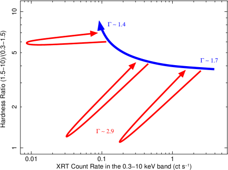
Figure 10: Schematic interpretation of the hardness-intensity plots. The fast decline during the first 3 months is associated to a moderate hardening (from $\Gamma\approx 1.7$–$1.8$ to $\Gamma\approx 1.4$) followed by a plateau. At early stages, the spectrum becomes much softer during each dip; at later times, the hardness ratio does not change in the dips.

Parameter	Band 1 Value	Band 2 Value	Band 3 Value	Band 4 Value	Band 5 Value
Model: tbabs*ztbabs*power-law
$N_{\rm H,Gal}$	$[0.02]$	$[0.02]$	$[0.02]$	$[0.02]$	$[0.02]$
$N_{{\rm H},z=0.354}$	$1.57^{+0.10}_{-0.10}$	$1.41^{+0.09}_{-0.09}$	$1.35^{+0.06}_{-0.06}$	$1.32^{+0.14}_{-0.12}$	$1.46^{+0.44}_{-0.35}$
$\Gamma$	$1.67^{+0.06}_{-0.06}$	$1.72^{+0.06}_{-0.06}$	$1.69^{+0.04}_{-0.04}$	$1.82^{+0.09}_{-0.09}$	$2.87^{+0.47}_{-0.40}$
$N_{\rm po}$	$16.6^{+1.4}_{-1.2}$	$12.0^{+1.0}_{-0.9}$	$8.2^{+0.4}_{-0.4}$	$3.5^{+0.4}_{-0.4}$	$1.8^{+1.1}_{-0.6}$
$f_{0.3-10}$	$7.7^{+0.1}_{-0.2}$	$5.3^{+0.1}_{-0.1}$	$3.8^{+0.1}_{-0.1}$	$1.3^{+0.1}_{-0.1}$	$0.20^{+0.02}_{-0.04}$
$L_{0.3-10}$	$46.8^{+1.3}_{-2.4}$	$32.4^{+1.4}_{-1.3}$	$22.5^{+0.6}_{-0.4}$	$8.9^{+0.6}_{-0.5}$	$5.8^{+4.0}_{-2.8}$
$\chi^{2}_{\nu}$	$1.06$	$0.96$	$0.96$	$0.98$	$1.03$
	$(328.3/311)$	$(271.1/282)$	$(461.1/480)$	$(155.2/158)$	$(26.8/26)$

Table 2: Best-fitting spectral parameters for de-trended intensity-selected Swift/XRT-PC spectra. Band 1 is for time intervals when the count rate was $>9/10$ of the spline-fitted baseline rate (Figure 1); band 2 for count rates between $2/3$ and $9/10$; band 3 for count rates between $1/3$ and $2/3$; band 4 for count rates between $1/10$ and $1/3$; band 5 for count rates $<1/10$ of the baseline. All bands include only intervals at $2\times 10^{5}~{}{\rm s}<t<9\times 10^{6}$ s. Units: $N_{\rm H,Gal}$ and $N_{{\rm H},z=0.354}$ are in units of $10^{22}$ cm^-2; $N_{\rm po}$ in $10^{-3}$ photons keV^-1 cm^-2 s^-1 at 1 keV; $f_{0.3-10}$ in $10^{-11}$ erg cm^-2 s^-1; $L_{0.3-10}$ in $10^{45}$ erg s^-1. Errors indicate the 90% confidence interval for each parameter of interest.

Parameter	Band A Value	Band B Value	Band C Value	Band D Value
Model: tbabs*ztbabs*power-law
$N_{\rm H,Gal}$	$[0.02]$	$[0.02]$	$[0.02]$	$[0.02]$
$N_{{\rm H,z}=0.354}$	$1.50^{+0.07}_{-0.09}$	$1.54^{+0.19}_{-0.20}$	$1.79^{+0.06}_{-0.09}$	$1.92^{+0.39}_{-0.34}$
$\Gamma$	$1.77^{+0.05}_{-0.05}$	$1.41^{+0.11}_{-0.11}$	$1.40^{+0.03}_{-0.04}$	$1.50^{+0.18}_{-0.17}$
$N_{\rm po}$	$30.2^{+1.8}_{-1.6}$	$1.6^{+0.3}_{-0.2}$	$1.3^{+0.1}_{-0.1}$	$1.0^{+0.3}_{-0.2}$
$f_{0.3-10}$	$12.2^{+0.1}_{-0.2}$	$1.1^{+0.1}_{-0.1}$	$0.91^{+0.05}_{-0.05}$	$0.54^{+0.04}_{-0.07}$
$L_{0.3-10}$	$80.8^{+2.7}_{-2.9}$	$5.7^{+0.3}_{-0.3}$	$4.5^{+0.1}_{-0.1}$	$3.2^{+0.2}_{-0.2}$
$\chi^{2}_{\nu}$	$1.06$	$0.90$	$0.92$	$1.06$
	$(432.3/408)$	$(95.6/106)$	$(487.5/528)$	$(78.4/74)$

Table 3: Best-fitting spectral parameters for time-selected Swift/XRT-PC spectra. All spectra include only intervals in which the count rate was $>2/3$ of the normalized continuum rate. Band A is for time intervals $2\times 10^{5}~{}{\rm s}<t<4.7\times 10^{6}$ s; band B for $4.7\times 10^{6}~{}{\rm s}<t<9\times 10^{6}$ s; band C for $9\times 10^{6}~{}{\rm s}<t<1.25\times 10^{7}$ s; band D for $1.25\times 10^{7}~{}{\rm s}<t<2.1\times 10^{7}$ s; Units are as in Table 1. Errors indicate the 90% confidence interval for each parameter of interest.

3.3.2 Spectral evolution

Our investigation of hardness evolution makes it clear that we need to distinguish between the short-term and long-term spectral evolution. To do so, we use the same method applied to our structure function analysis: we normalised the snapshot light-curve to a smooth empirical function that fits the long-term evolution. We then extracted intensity-selected spectra based on the normalised count rates rather than the observed ones; for example, integrated spectra from all time intervals in which the normalised flux was $>0.9$, or between $2/3$ and $0.9$, etc. We also fixed the flux level and extracted time-selected spectra, that is with the same normalised flux band but at different epochs.

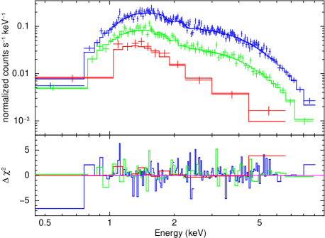
Figure 11: Best-fitting power-law models and $\chi^{2}$ residuals for three de-trended intensity-selected spectra, showing spectral steepening in the dips. Blue datapoints and residuals: background-subtracted spectrum extracted from all the time intervals when the count rate was $>9/10$ times the de-trended baseline (Band 1 in Table 2). Green datapoints and residuals: spectrum from the time intervals when the count rate was between $1/10$ and $3/10$ of the de-trended baseline (Band 4 in Table 2). Red datapoints and residuals: spectrum from the time intervals when the count rate was $\leq 0.1$ times the de-trended baseline (Band 5 in Table 2). For all three spectra, we used only data up to $t=9\times 10^{6}$ s; we used only data in PC mode, to reduce background contamination. See Table 2 for the fit parameters.

In Table 2, we summarise the result of spectral fitting for a sample of intensity-selected spectra from the decline phase ($t<9\times 10^{6}$ s). All spectra are well fitted by absorbed power-laws, with a column density $\sim 1.5\times 10^{22}$ cm^-2 in the local frame at redshift 0.354. Small variations in the fitted column density from band to band may not be statistically significant, and do not appear to follow any trend. The high- and medium-intensity bands have a similar photon index $\approx 1.7$. Low-intensity bands have a steeper slope, as already suggested by our hardness ratio analysis: as steep as $\Gamma\approx 2.9$ for spectra taken across the bottom of the dips (Figure 11). This result confirms our interpretation of the hardness-intensity plots and is consistent with the spectral results of Miller & Strohmayer (2011). It shows even more clearly that the early dips are characterised by a steeper spectral slope, not by higher absorption: they are not eclipses by orbiting or rotating clouds.

We then considered high- and medium-intensity spectra (which, as we have seen from Table 2, have the same average spectral slope), taken from all time intervals with normalised count rates $>2/3$, and divided them into several time bands corresponding to the intervals used for timing analysis. We found (Table 3) that all spectra are well fitted by a simple absorbed power-law; adding blackbody or optically thin thermal components does not improve the fit, nor is there any evidence of breaks in the power-law at high energies. The slope in the early epoch ($t<4.7\times 10^{6}$ s) was $\Gamma\approx 1.8$, flattening to $\Gamma\approx 1.4$–$1.5$ at later epochs (Figure 12). This long-term spectral trend is in perfect agreement with what was inferred from the hardness-intensity study (§ 3.3.1 and Figure 10). The intrinsic column density appears to increase at later epochs (Table 3), although this result is only marginally significant.

At late epochs, the unabsorbed isotropic $0.3$–$10$ keV luminosity becomes as low as $\approx 4\times 10^{44}$ erg s^-1 during the dips (Table 4). This is now approaching the pre-burst upper limit to the X-ray luminosity, $L_{\rm X}\la 1.7\times 10^{44}$ erg s^-1 (Bloom et al., 2011b). If Sw J1644$+$57 continues its decline, it is plausible that in a few months’ time we will start seeing the unbeamed component of the emission (e.g., from an accretion disk or its corona), or we will infer stronger limits on the unbeamed flux. We tried fitting the late-epoch dip spectrum with a thermal-plasma model and found that it is at least as good as a power-law model (Table 4); there are not enough counts to discriminate between them.

Parameter	Value 1	Value 2
Model 1: tbabs*ztbabs*power-law
Model 2: tbabs*ztbabs*raymond-smith
$N_{\rm H,Gal}$	$[0.02]$	$[0.02]$
$N_{{\rm H,z}=0.354}$	$1.8^{+1.6}_{-1.3}$	$1.7^{+1.2}_{-0.9}$
$\Gamma$	$1.58^{+0.73}_{-0.70}$	–
$N_{\rm po}$	$0.14^{+0.07}_{-0.07}$	–
$kT_{\rm e}$	–	$>3.9$
$N_{\rm rs}$	–	$7.8^{+5.0}_{-1.9}$
$f_{0.3-10}$	$0.073^{+0.013}_{-0.012}$	$0.064^{+0.011}_{-0.032}$
$L_{0.3-10}$	$0.45^{+0.30}_{-0.10}$	$0.39^{+0.08}_{-0.04}$
Cstat	$7.35/12$	$6.16/12$

Table 4: Best-fitting spectral parameters for the Swift/XRT-PC spectrum during the late dips ($1.25\times 10^{7}~{}{\rm s}<t<2.1\times 10^{7}$ s), fitted with the standard power-law model and with an optically-thin thermal plasma model. Units of $N_{\rm H}$, flux and luminosity are as in Table 2. The normalisation $N_{\rm rs}=10^{-11}(1+z)^{2}/(4\pi\,D^{2})\int(n_{\rm e}n_{\rm I}dV)$ where $D$ is the luminosity distance. Errors indicate the 90% confidence interval for each parameter of interest.

4 Discussion

The general consensus is that Sw J1644$+$57 is a previously quiescent nuclear BH that underwent an outburst caused by accretion of a tidally disrupted star (Bloom et al., 2011a, b; Burrows et al., 2011; Cannizzo, Troja & Lodato, 2011; Socrates, 2011). Its high apparent luminosity requires strong beaming. The emission in the keV band can be explained as synchrotron and/or inverse Compton radiation from energetic electrons streaming along the relativistic jet pointing towards us. The relative contribution of the two processes is still debated. It is also still unclear how the jets are launched at the onset of the outburst, when a fully formed accretion disc cannot have had the time to develop, after the disruption event (cf. the violent mass transfer and jet formation in the X-ray binary Cir X-1; Johnston, Fender & Wu, 1999).

From the Swift/XRT data we have extracted further information on the time-dependent behaviour and spectral evolution of the source. We have decomposed the amplitude variations into a long-term evolution (an initial decline followed by a plateau) and recurrent dips. If these dips had been wholly stochastic processes, we would expect that fluctuations should be of the same order of magnitude as the depths of the dips. Otherwise it would require many miniature flares (a day’s worth of them) to coherently conspire to become small simultaneously, or to abstain simultaneously.

However we have shown that the dips are not merely random fluctuations (as is often the case in the X-ray light-curve of accreting sources), but have a certain regularity, apparently governed by an underlying periodic driver. We have used Lomb-Scargle periodograms and structure function analysis to search for the main characteristic timescales in the frequency range $\sim 10^{-7}$–$10^{-4}$ Hz. We expect variability on those timescales based on physical arguments. For example, there may be a residual inhomogeneous distribution of debris at or near the tidal disruption radius $R_{\rm TD}\approx 10GM_{\bullet}/c^{2}\times[M_{\bullet}/(10^{7}M_{\odot})]^{-2/3}$ (for a solar-type star). The Keplerian timescale $t_{\rm K}=2\pi/\Omega_{\rm K}$ at the tidal disruption radius is $\approx 10^{4}$ s (Rees, 1988), independent of BH mass in the Newtonian approximation. The ring of debris is likely to be still oriented in the orbital plane of the disrupted star: this may generate a Lense-Thirring precession with a timescale $t_{\rm LT}=[t_{\rm K}/(2a)]\times[(R_{\rm TD}c^{2})/(GM_{\bullet})]^{3/2}\sim 30$–$300t_{\rm K}/(2a)\sim 10^{5}$–$10^{6}$ s (Armitage & Natarajan, 1999; Merritt et al., 2010; Stone & Loeb, 2012), where $a$ is the BH spin parameter. We found significant features in the Lomb-Scargle periodograms and structure functions, especially at $\tau\approx 2.3$ Ms, 4.5 Ms, 9 Ms during the early epochs, and $\tau\approx 0.7$ Ms and 1.4 Ms during the late epochs. It appears that the characteristic dipping timescale (and its associated harmonics) has shifted between the early and late section of the lightcurve.

Whatever the mechanism for the dips, it is something that also changes the spectral properties of the emission, as the spectrum is steeper during the early dips ($\Gamma\approx 2.8$–$3$) than immediately before and after ($\Gamma\approx 1.4$–$1.7$). At the same time, the long-term trend outside the dips shows spectral hardening at the beginning, followed by a plateau at $\Gamma\approx 1.4$.

Figure 12: Best-fitting power-law models and $\chi^{2}$ residuals for three time-selected spectra, showing moderate long-term hardening. Red datapoints and residuals: background-subtracted spectrum extracted from the time interval $2\times 10^{5}~{}{\rm s}<t<4.7\times 10^{6}$ s and only including intervals with a count rate $>2/3$ times the de-trended baseline. Green datapoints and residuals: background-subtracted spectrum at $4.7\times 10^{6}~{}{\rm s}<t<9\times 10^{6}$ s and count rate $>2/3$. Blue datapoints and residuals: background-subtracted spectrum at $9\times 10^{6}~{}{\rm s}<t<1.25\times 10^{7}$ s and count rate $>2/3$. All data are in PC mode. See Table 3 for the fit parameters.

Here, we attempt to make sense of our findings in the framework of a synchrotron-emitting relativistic jet scenario. We propose that: (i) the jets have precessional and nutational motion; (ii) the jets have a collimated core surrounded by an envelope of less energetic, less collimated electrons straying out of the core; (iii) the synchrotron-emitting jets become more compact as the source declines, after the initial outburst.

In this scenario, the baseline flux in the XRT band is direct synchrotron emission from a jet pointing toward us. In the first few days after the outburst, when the accretion rate is highest, the jet expands and propagates forward into the interstellar medium. The X-ray emission region is most extended at that early epoch, and it is optically thin to synchrotron radiation. Energetic electrons are freshly accelerated in the jets, with an energy distribution $N(E)\propto E^{-p}$, where the energy spectral index $2.2\la p\la 2.5$ (see e.g., Ballard & Heavens, 1992; Kirk & Duffy, 1999). The synchrotron emission spectrum from this population of electrons has a specific intensity $I_{\nu}\propto\nu^{-\alpha}$ with $\alpha\approx 0.7$, corresponding to a photon index $\Gamma\approx 1.7$. When the most violent flarings subside and accretion becomes more steady, the overall accretion luminosity of the system decreases and the jet power is reduced accordingly. In this phase, synchrotron emission no longer comes from the expanding jet ejecta, but it is rather confined to the vicinities of shocks at the base of the jet. As the X-ray emission region becomes more compact and denser, the synchrotron photons start to suffer self-absorption, leading to the observed spectral flattening: approaching a similar situation to the flat-spectrum core emission in radio galaxies with compact jets.

Moreover, the transition from extended to compact jet emission may also provide a simple explanation for the levelling off of the X-ray luminosity at late epochs. For an optically thin source, the luminosity depends on the total volume of the synchrotron-emitting region in the jets; a constant luminosity would require a high degree of fine-tuning. By contrast, in an opaque source, the luminosity depends on the effective area of the emission region visible to us. The growth of the radio emitting region is perhaps explained by a more diffuse outer region, such as the larger jet-driven turbulent cocoon and the expanding bow shock surrounding the whole system (Bower, Bloom & Cenko, 2011; Zauderer et al., 2011; Burrows et al., 2011). Modelling the radio flux evolution requires knowledge of the jet parameters, which are unfortunately not well constrained by the observational data obtained so far. We therefore leave the jet modelling, which is beyond the scope of this paper, to a future study.

Regarding the dips, we showed that they are not due to partial occultation of the jets by some line-of-sight material, as we would expect higher absorption rather than spectral steepening in this situation, contrary to what is observed. Instead we propose that dips occur when the synchrotron-emitting jet is not perfectly aligned along our line-of-sight, and hence the most highly beamed component of the synchrotron emission does not reach us. The observed X-ray flux is then dominated by the lower level of emission from the slower and/or less collimated electrons in a sheath or cocoon around the jet. This emission could be synchrotron from an aged (steeper-spectrum) population of electrons, if there are significant magnetic fields in the jet envelope, or synchrotron self-Compton. We must also stress that even at the bottom of the dips, the apparent luminosity is higher or similar (for the late dips) to the Eddington luminosity of a $10^{7}M_{\odot}$ BH. This suggests that the emission is moderately beamed even during the dips.

In addition to the expected long-term decline and stochastic flux variability, it is intriguing that many of the dips occur on regular patterns, likely to be governed by a periodic driver; it is even more intriguing that sometimes a dip is skipped but the following one happens again approximately at the expected phase (Figure 4). Careful inspection of the centroid locations of the dips has revealed that they are not exactly phase-matched but can be slightly advanced or delayed. To explain these peculiar dip patterns, we propose that the jet undergoes nutation as well as precession. The combination of the two effects drives the cone of the jet out of our line of sight, from time to time. The presence of nutation is essential, as it naturally explains why the dips occur in a regular but not exactly periodic pattern, and why there are slight advances or delays of the dip centroids.

We note also that the appearance of the dips changes: in the early epoch we see a slow fainting and rapid rise; but in later dips the dimming and rising are symmetric (Figure 4). The fractional time that the object is in a dip or out of a dip also changes: brief dips at early times; long dips in late epochs. These observations gain significance in the jet precession/nutation scenario, especially if the emission core became more compact. When the early dips were sharp and brief, the precession subtended a tight angle, compared to the jet’s beaming angle. The larger width of the dips at late times, and the larger fraction of time spent in a dip, probably indicates that the core of the jet is narrower (or swinging more widely) while the layer of slower electrons around the core grows in size. The asymmetric dipping at early times may mean that the region around the core is not moving in phase with the jet core; lagging while the core moves out of the line of sight, while being compacted when the core moves back.

The remaining question is what causes the jet precession and nutation. Jet precession is expected as the BH spin axis is unlikely to be perfectly aligned with the initial angular momentum of the disrupted star. Thus, the normal direction to the plane of the transient accretion ring/disc formed by the stellar debris is tilted with respect to the BH spin, and this causes the jet to precess. In addition, jet nutation can be triggered if the precessing jet/disc system has been perturbed, either by an internal or external driver. In the internally driven case, nutation may be induced by an uneven mass distribution in the transient debris ring/disc. In the externally driven case, the jet and the accretion ring/disc may be perturbed by the orbiting remnant of the partially disrupted star — for example, a white dwarf on an elliptical orbit would make several passes inside the tidal radius before being completely disrupted (Krolik & Piran, 2011). Alternatively, they may be perturbed by another gravitating object, such as (unlikely but not impossible) a satellite massive black hole (as predicted in nuclear swarms of compact objects: Freitag, Amaro-Seoane & Kalogera, 2006; Portegies Zwart et al., 2006); or perhaps a more supermassive companion (about which Sw J1644$+$57 is the satellite).

An important clue to the evolution of the system comes from the change in the characteristic variability timescales at early and late times. If the nutation is externally driven, the change of period might conceivably be explained if the torque changed (perhaps during an eccentric perimelasma passage). Scenarios dominated by disc torques suggest other possibilities. A possible explanation is that the warped disk has not yet reached a steady state or Bardeen-Petterson regime (Bardeen & Petterson, 1975; Kumar & Pringle, 1985). In other words, the warp radius (transition between the inner part of the disc aligned with the BH spin and the outer part aligned with the orbital plane of the mass donor) may still be propagating outwards, and as a result the Lense-Thirring precession timescale at the warp radius is increasing. Alternatively, it was suggested (Fragile et al., 2007; Dexter & Fragile, 2011; Stone & Loeb, 2012) that a geometrically thick disc may never settle in a Bardeen-Petterson regime, and may instead precess as a solid body (a tilted, rather than warped disc). In this case, the precession frequency depends on the dimensionless radial surface density profile of the disc, which is also likely to evolve in time.

In fact, a problem of the disc-driven precessing-jet scenario is that we expect the jet axis to have already precessed out of alignment with our line of sight (and not just for short dips) after few weeks, unless the initial alignment of disc and BH spin axis was already very close (Stone & Loeb, 2012). This seems an unlikely coincidence if the disc was formed after a tidal disruption event. Thus, we suggest a note of caution regarding the tidal disruption scenario as the origin of the flare. It is useful to remember that the 2011 March 28 flare marks the moment when the jet turned on, not the time of the putative tidal disruption event, which may have happened unobserved several weeks earlier, depending on the time required to spread the debris onto a disc, build up a magnetic field and launch a jet. The main argument for a tidal disruption as the origin of the whole process is that the host galaxy was not known as an AGN before the flare. However, pre-event luminosity upper limits (Bloom et al., 2011b) are only implying that the bolometric luminosity was below Eddington for a $10^{7}M_{\odot}$ BH, or below $10$ Eddington for a $10^{6}M_{\odot}$ BH. Thus, we cannot exclude that an accretion disc was already present and approximately aligned, and the jet ejection was due to a state transition rather than a tidal disruption. State transitions with relativistic blob ejections and radio/X-ray flares are common in Galactic BH transients, especially when they switch from the hard to the soft (thermal) state (Fender, Belloni & Gallo, 2004; Fender & Belloni, 2004). Scaled with their respective mass ranges, the duration of the flare in Sw J1644$+$57 so far corresponds to only $\sim 10$–$100$ s in a typical Galactic BH. Further monitoring of the flux evolution over the next few months will help testing between the tidal disruption and state transition scenarios.

The scenario outlined above does not imply that every dip is due to oscillations and precession of the jet. Our most general interpretation is that dips correspond to phases when we are seeing slower and less collimated electrons along our line of sight in the jet. Even when the nozzle is steady, jets are subject to internal instabilities of magneto-hydro-dynamical nature. Internal shocks echo and self-intersect up and down the jet, producing standing patterns with a characteristic spacing that depends on the Mach number of the flow and the width of the jet. Jets also suffer an axisymmetric pinch instability, a non-asxisymmetric helical instabilities, and other higher-order harmonics of the helical instability (Hardee & Norman, 1988; Norman & Hardee, 1988; Hardee et al., 1992). Observed changes in the jet collimation and luminosity will depend on the interplay of the external driving oscillations (e.g., jet precession) and the resonant frequencies of the internal instabilities. The situation becomes even more complex if — as seems to be the case in Sw J1644$+$57 (Berger et al., 2011) — the jet has a broad Lorentz factor distribution rather than a single speed. With more arduously detailed modelling work (in the future), tested by long-term X-ray and radio monitoring (Berger et al., 2011), one might hope to infer something about the internal layering of the jet, and distinguish between internal and external driven jet variability.

5 Conclusion

We investigated the luminosity and spectral evolution of the peculiar X-ray source Sw J1644$+$57 using Swift/XRT data. Our structure function analysis showed that the large-amplitude variations in the light curve of the source are not simply stochastic fluctuations. In particular, the occurrence of at least some of the dips appears to follow some regular patterns characterised by multiples and fractions of a time interval $\tau\approx 4.5\times 10^{5}$ s; visually, several prominent dips are spaced at $\approx 0.5\tau\approx 2.2\times 10^{5}$ s, and $\approx 2\tau\approx 9\times 10^{5}$ s. After the plateau the base period switched to $\tau\approx 1.4\times 10^{6}$ s, but the scenario remains essentially the same. The X-ray spectrum outside the dips is always consistent with an absorbed power-law, but its photon index evolves on a weekly/monthly timescale, from $\Gamma\approx 1.8$ at the beginning of the decline phase to $\Gamma\approx 1.4$ at a later stage when the luminosity seems to level off. The X-ray spectrum is much softer during the dips, while there is no significant change in the absorption column density.

We proposed a scenario in which the synchrotron emitting jets, launched from a massive BH accreting a disrupted star, undergo both precession and nutation. The baseline flux in the keV band is direct synchrotron emission when the jet cone is in our line of sight; dips occur when the jet cone goes briefly and partially out of our line of sight. We argued that the synchrotron photons come from the optically thin jet ejecta during the initial high-luminosity, exponential decay phase; as the accretion power subsides, the dominant emission region becomes an opaque feature that is confined to a compact jet core. We attributed the fainter, steep-spectrum dip emission to a population of less energetic electrons, perhaps streaming in a cocoon surrounding the collimated jet core. Jet nutation and precession provide a natural explanation for the dip patterns in the X-ray light-curve: in particular, their preferred occurrence at some regular intervals, their occasional disappearance and subsequent reappearance, and the phase advance and delay of the dip centroids. In addition, internal jet instabilities can produce oscillations in the speed and cross section of the jet flow, and therefore a recurrent dipping behaviour. Long-term monitoring of the characteristic oscillation frequencies will be required to test whether they are due to internal or external drivers.

Appendix

A.1 Piecewise linear light curves

Consider a temporally evolving signal $z$ (e.g. X-ray flux or counts), for which the data occur in bins $i$ spanning temporal intervals $[t_{i},u_{i}]$ where $t_{i}$ is the starting time and $u_{i}$ is the ending time of bin $i$. In characterising the temporal variability of the light-curve, we may offset a copy of these bins by a lag time $\tau$, and compare to the unoffset data. With patchy, piecewise data, it is necessary to compute the temporal overlap between each pair of unoffset and offset bins. If the time intervals of the offset bins are $[t_{j}^{\prime},u_{j}^{\prime}]=[t_{j}+\tau,u_{j}+\tau]$, then the interval of overlap with an unoffset bin $[t_{i},u_{i}]$ is $[T_{ij},U_{ij}]=[\max(t_{i},t_{j}^{\prime}),\min(u_{i},u_{j}^{\prime})]$. If $U_{ij}<T_{ij}$, then there is no overlap. The weight or duration of overlap between a pair of bins $i,j$ is

$$w_{ij}=w_{ij}(\tau)=\left\{{\begin{array}[]{ll}U_{ij}-T_{ij}&\mbox{if $U_{ij}\geq T_{ij}$,}\\ 0&\mbox{otherwise.}\end{array}}\right.\ .$$ (2)

Suppose that the amplitudes within each bin evolve linearly in time: $z=a_{i}\,t+b_{i}$ and $z^{\prime}=a_{j}\,t+b_{j}$. The linear coefficients depend on the (observed) amplitudes $z$ and times at the ends of each time interval, $a_{j}=({{\delta z_{j}})/({u_{j}-t_{j}}})$ and $b_{j}=z_{j}-a_{j}t_{j}$. During the overlap, the difference between the amplitudes of offset and unoffset light curves is $y\equiv z_{j}^{\prime}(t+\tau)-z_{i}(t)=A_{ij}\lambda+B_{ij}$, with $\lambda\equiv(t-T_{ij})/(U_{ij}-T_{ij})$, and $0\leq\lambda\leq 1$ by construction, where we abbreviate

$$A_{ij}=(\nu_{ij}^{\prime}-\mu_{ij}^{\prime})\delta z_{j}-(\nu_{ij}-\mu_{ij})\delta z_{i}\ ;$$ (3)

$$B_{ij}=\mu_{ij}^{\prime}\delta z_{j}+b_{j}+a_{j}t_{j}-\mu_{ij}\delta z_{i}-b_{i}-a_{i}t_{i}\ .$$ (4)

For brevity, we define relative fractions $\mu_{ij}$, $\nu_{ij}$, $\mu_{ij}^{\prime}$, and $\nu_{ij}^{\prime}$ expressing how far the overlap occurs along the segments $i$ and $j$.

$$\mu_{ij} \equiv {{T_{ij}-t_{i}}\over{u_{i}-t_{i}}}\ ;$$

$$\nu_{ij} \equiv {{U_{ij}-t_{i}}\over{u_{i}-t_{i}}}\ ;$$

$$\mu_{ij}^{\prime} \equiv {{T_{ij}+\tau-t_{j}}\over{u_{j}-t_{j}}}\ ;$$

$$\nu_{ij}^{\prime} \equiv {{U_{ij}+\tau-t_{j}}\over{u_{j}-t_{j}}}\ .$$ (5)

A2. Structure functions for unevenly sampled data

For continuous data, the order-$n$ structure function is defined as

$$S_{n}(\tau) \equiv \left\langle\left[{z(t+\tau)-z(t)}\right]^{n}\right\rangle$$ (6)

$$= \frac{1}{\mathcal{T}}\int_{\mathcal{T}}[z(t+\tau)-z(t)]^{n}\,{\mathrm{d}}t\ .$$

For patchy, discretely binned data, we need to integrate contributions from each pair of potentially overlapping bins, piece by piece. If bin $i$ overlaps with the offset copy of bin $j$ then this pair contributes an amount $I_{ij}$ to the numerator of the structure function,

$$I_{ij} = I_{ij}(\tau)=\int_{T_{ij}}^{U_{ij}}\left[{z^{\prime}(t+\tau)-z(t)}\right]^{n}\,{\mathrm{d}}t$$ (7)

$$= \int_{T_{ij}}^{U_{ij}}\left[{a_{j}\,t+a_{j}\,\tau+b_{j}-a_{i}\,t-b_{i}}\right]^{n}\,{\mathrm{d}}t\ ,$$

so that $S_{n}=S_{n}(\tau)=W^{-1}\sum_{ij}I_{ij}$. The normalisation factor $W$ is the total duration of temporal overlaps between all pairs of bins.

$$W\equiv\sum_{i,j}w_{ij}\ .$$ (8)

For $a_{i}\neq a_{j}$ (and $A_{ij}\neq 0$), the integral (7) can be evaluated directly,

$$I_{ij} = w_{ij}\int_{0}^{1}\,y^{n}\,{\mathrm{d}}\lambda$$ (9)

$$= {{w_{ij}}\over{(n+1)A_{ij}}}\left[{(A_{ij}+B_{ij})^{n+1}-B_{ij}^{n+1}}\right]\ .$$

An alternative, binomial expansion proves to be more numerically stable in practice, especially where $|A_{ij}|$ is small:

$$I_{ij}=w_{ij}\sum_{k=0}^{n}{n\choose k}{{A_{ij}^{k}B_{ij}^{n-k}}\over{k+1}}\ .$$ (10)

A3. Determination of the uncertainties

If each bin $k$ has a measurement $z_{k}$, with uncertainty $\Delta z_{k}$, then we obtain the uncertainty on the overall structure function by quadrature. Now to propagate the uncertainties in the measurements $z_{k}$ to uncertainties in the structure functions $S_{n}(\tau)$, one needs partial derivatives of each piece $I_{ij}$ with respect to each observable $z_{k}$. It emerges that

$${{\partial I_{ij}}\over{\partial z_{k}}} = w_{ij}\sum_{k=0}^{n}{n\choose k}\biggl{[}{k\over{k+1}}A_{ij}^{k-1}B_{ij}^{n-k}{{\partial A_{ij}}\over{\partial z_{k}}}$$ (11)

$$\hskip 56.9055pt+{{n-k}\over{k+1}}A_{ij}^{k}B_{ij}^{n-k-1}{{\partial B_{ij}}\over{\partial z_{k}}}\biggr{]}\ .$$

If we assume a zigzag data patching scheme ($z_{i+1}=z_{i}+\delta z_{i}$) then the revelant partial derivatives of $A_{ij}$ and $B_{ij}$ are

$${{\partial A_{ij}}\over{\partial z_{k}}} = \hskip 7.11317pt(\nu_{ij}^{\prime}-\mu_{ij}^{\prime})\delta_{{}_{k,j+1}}-(\nu_{ij}^{\prime}-\mu_{ij}^{\prime})\delta_{{}_{k,j}}$$ (12)

$$-(\nu_{ij}-\mu_{ij})\delta_{{}_{k,i+1}}+(\nu_{ij}-\mu_{ij})\delta_{{}_{k,i}}\ ;$$

$${{\partial B_{ij}}\over{\partial z_{k}}} = \hskip 8.53581pt\mu_{ij}^{\prime}\delta_{{}_{k,j+1}}+(1-\mu_{ij}^{\prime})\delta_{{}_{k,j}}$$ (13)

$$-\mu_{ij}\delta_{{}_{k,i+1}}+(\mu_{ij}-1)\delta_{{}_{k,i}}\ ,$$

where $\delta$ is the Kronecker delta symbol. Now abbreviate

$${\mathcal{A}}_{ij} \equiv w_{ij}\sum_{k=0}^{n}{n\choose k}{{k}\over{k+1}}A_{ij}^{k-1}B_{ij}^{n-k}\ ;$$ (14)

$${\mathcal{B}}_{ij} \equiv w_{ij}\sum_{k=0}^{n}{n\choose k}{{n-k}\over{k+1}}A_{ij}^{k}B_{ij}^{n-k-1}\ ,$$ (15)

and

$$C_{1_{ij}} = {\mathcal{A}}_{ij}(\nu_{ij}^{\prime}-\mu_{ij}^{\prime})+{\mathcal{B}}_{ij}\mu_{ij}^{\prime}\ ;$$ (16)

$$C_{2_{ij}} = -{\mathcal{A}}_{ij}(\nu_{ij}^{\prime}-\mu_{ij}^{\prime})+{\mathcal{B}}_{ij}(1-\mu_{ij}^{\prime})\ ;$$ (17)

$$C_{3_{ij}} = -{\mathcal{A}}_{ij}(\nu_{ij}-\mu_{ij})-{\mathcal{B}}_{ij}\mu_{ij}\ ;$$ (18)

$$C_{4_{ij}} = {\mathcal{A}}_{ij}(\nu_{ij}-\mu_{ij})+{\mathcal{B}}_{ij}(\mu_{ij}-1)\ .$$ (19)

It follows that

$${{\partial I_{ij}}\over{\partial z_{k}}}=C_{1_{ij}}\delta_{{}_{k,j+1}}+C_{2_{ij}}\delta_{{}_{k,j}}+C_{3_{ij}}\delta_{{}_{k,i+1}}+C_{4_{ij}}\delta_{{}_{k,i}}\ .$$ (20)

By contracting the Kronecker deltas, we obtain

$${{\partial S_{n}}\over{\partial z_{k}}} = {1\over{W}}\sum_{ij}{{\partial I_{ij}}\over{\partial z_{k}}}$$ (21)

$$= {1\over{W}}\sum_{i}\left({C_{1_{i,k-1}}+C_{2_{i,k}}+C_{3_{k-1,i}}+C_{4_{k,i}}}\right)\ .$$

The four matrices (${\sf C}_{1},{\sf C}_{2},{\sf C_{3}},{\sf C}_{4}$) only need to be computed once for each choice of $\tau$. If the uncertainties in the flux measurements are $\Delta z_{k}$, the total uncertainty in the structure function is then given by

$$\left({\Delta S_{n}}\right)^{2}=\sum_{k}\left({{{\partial S_{n}}\over{\partial z_{k}}}\Delta z_{k}}\right)^{2}\ .$$ (22)

References

- Armitage & Natarajan (1999) Armitage P. J., Natarajan P., 1999, ApJ, 525, 909
- Arnaud (1996) Arnaud K. A., 1996, in Astronomical Society of the Pacific Conference Series, Vol. 101, Astronomical Data Analysis Software and Systems V, G. H. Jacoby & J. Barnes, ed., pp. 17–
- Ballard & Heavens (1992) Ballard K. R., Heavens A. F., 1992, MNRAS, 259, 89
- Bardeen & Petterson (1975) Bardeen J. M., Petterson J. A., 1975, ApJ, 195, L65
- Barthelmy et al. (2005) Barthelmy S. D. et al., 2005, Space Sci. Rev., 120, 143
- Bennert et al. (2011) Bennert V. N., Auger M. W., Treu T., Woo J.-H., Malkan M. A., 2011, ApJ, 726, 59
- Berger et al. (2011) Berger E., Zauderer A., Pooley G. G., Soderberg A. M., Sari R., Brunthaler A., Bietenholz M. F., 2011, ArXiv e-prints, 1112.1697
- Blackburn (1995) Blackburn J. K., 1995, in Astronomical Society of the Pacific Conference Series, Vol. 77, Astronomical Data Analysis Software and Systems IV, R. A. Shaw, H. E. Payne, & J. J. E. Hayes, ed., pp. 367–
- Bloom et al. (2011a) Bloom J. S., Butler N. R., Cenko S. B., Perley D. A., 2011a, GRB Coordinates Network, 11847, 1
- Bloom et al. (2011b) Bloom J. S. et al., 2011b, Science, 333, 203
- Boldyrev, Nordlund & Padoan (2002) Boldyrev S., Nordlund Å., Padoan P., 2002, Physical Review Letters, 89, 031102
- Bower, Bloom & Cenko (2011) Bower G., Bloom J., Cenko B., 2011, The Astronomer’s Telegram, 3278, 1
- Brandenburg & Nordlund (2011) Brandenburg A., Nordlund Å., 2011, Reports on Progress in Physics, 74, 046901
- Bregman et al. (1988) Bregman J. N. et al., 1988, ApJ, 331, 746
- Brinkmann et al. (2000) Brinkmann W., Gliozzi M., Urry C. M., Maraschi L., Sambruna R., 2000, A&A, 362, 105
- Brinkmann et al. (2001) Brinkmann W. et al., 2001, A&A, 365, L162
- Burrows et al. (2005) Burrows D. N. et al., 2005, Space Sci. Rev., 120, 165
- Burrows et al. (2011) Burrows D. N. et al., 2011, Nature, 476, 421
- Cannizzo, Troja & Lodato (2011) Cannizzo J. K., Troja E., Lodato G., 2011, ApJ, 742, 32
- Cenko et al. (2011) Cenko S. B. et al., 2011, ArXiv e-prints, 1107.5307
- Cordes & Downs (1985) Cordes J. M., Downs G. S., 1985, ApJS, 59, 343
- Cummings et al. (2011) Cummings J. R. et al., 2011, GRB Coordinates Network, 11823, 1
- Desidera et al. (2011) Desidera S. et al., 2011, A&A, 533, A90
- Dexter & Fragile (2011) Dexter J., Fragile P. C., 2011, ApJ, 730, 36
- Emmanoulopoulos, McHardy & Uttley (2010) Emmanoulopoulos D., McHardy I. M., Uttley P., 2010, MNRAS, 404, 931
- Evans et al. (2009) Evans P. A. et al., 2009, MNRAS, 397, 1177
- Evans et al. (2007) Evans P. A. et al., 2007, A&A, 469, 379
- Farrell et al. (2010) Farrell S. A., Gosling A. J., Webb N. A., Barret D., Rosen S. R., Sakano M., Pancrazi B., 2010, A&A, 523, A50
- Fender & Belloni (2004) Fender R., Belloni T., 2004, ARA&A, 42, 317
- Fender, Belloni & Gallo (2004) Fender R. P., Belloni T. M., Gallo E., 2004, MNRAS, 355, 1105
- Foullon, Verwichte & Nakariakov (2009) Foullon C., Verwichte E., Nakariakov V. M., 2009, ApJ, 700, 1658
- Fragile et al. (2007) Fragile P. C., Blaes O. M., Anninos P., Salmonson J. D., 2007, ApJ, 668, 417
- Freitag, Amaro-Seoane & Kalogera (2006) Freitag M., Amaro-Seoane P., Kalogera V., 2006, ApJ, 649, 91
- Gehrels et al. (2004) Gehrels N. et al., 2004, ApJ, 611, 1005
- Graham (2012) Graham A. W., 2012, ApJ, 746, 113
- Guidorzi (2011) Guidorzi C., 2011, MNRAS, 415, 3561
- Hakala et al. (2003) Hakala P., Ramsay G., Wu K., Hjalmarsdotter L., Järvinen S., Järvinen A., Cropper M., 2003, MNRAS, 343, L10
- Hardee et al. (1992) Hardee P. E., Cooper M. A., Norman M. L., Stone J. M., 1992, ApJ, 399, 478
- Hardee & Norman (1988) Hardee P. E., Norman M. L., 1988, ApJ, 334, 70
- Horne & Baliunas (1986) Horne J. H., Baliunas S. L., 1986, ApJ, 302, 757
- Hughes, Aller & Aller (1992) Hughes P. A., Aller H. D., Aller M. F., 1992, ApJ, 396, 469
- Iyomoto & Makishima (2001) Iyomoto N., Makishima K., 2001, MNRAS, 321, 767
- Jahnke & Macciò (2011) Jahnke K., Macciò A. V., 2011, ApJ, 734, 92
- Johnston, Fender & Wu (1999) Johnston H. M., Fender R., Wu K., 1999, MNRAS, 308, 415
- Kataoka et al. (2001) Kataoka J. et al., 2001, ApJ, 560, 659
- Kennea et al. (2011) Kennea J. A. et al., 2011, The Astronomer’s Telegram, 3250, 1
- Kirk & Duffy (1999) Kirk J. G., Duffy P., 1999, Journal of Physics G Nuclear Physics, 25, 163
- Kolmogorov (1941) Kolmogorov A., 1941, Akademiia Nauk SSSR Doklady, 30, 301
- Kolmogorov (1991) Kolmogorov A. N., 1991, Royal Society of London Proceedings Series A, 434, 9
- Kormendy, Bender & Cornell (2011) Kormendy J., Bender R., Cornell M. E., 2011, Nature, 469, 374
- Krimm & Barthelmy (2011) Krimm H. A., Barthelmy S. D., 2011, GRB Coordinates Network, 11891, 1
- Kritsuk et al. (2007) Kritsuk A. G., Norman M. L., Padoan P., Wagner R., 2007, ApJ, 665, 416
- Kritsuk et al. (2009) Kritsuk A. G., Ustyugov S. D., Norman M. L., Padoan P., 2009, in Astronomical Society of the Pacific Conference Series, Vol. 406, Astronomical Society of the Pacific Conference Series, N. V. Pogorelov, E. Audit, P. Colella, & G. P. Zank, ed., pp. 15–
- Krolik & Piran (2011) Krolik J. H., Piran T., 2011, ApJ, 743, 134
- Kumar & Pringle (1985) Kumar S., Pringle J. E., 1985, MNRAS, 213, 435
- Lauer et al. (2007) Lauer T. R. et al., 2007, ApJ, 662, 808
- Leahy et al. (1983) Leahy D. A., Darbro W., Elsner R. F., Weisskopf M. C., Kahn S., Sutherland P. G., Grindlay J. E., 1983, ApJ, 266, 160
- Levan et al. (2011a) Levan A. J. et al., 2011a, Science, 333, 199
- Levan et al. (2011b) Levan A. J., Tanvir N. R., Wiersema K., Perley D., 2011b, GRB Coordinates Network, 11833, 1
- Lin et al. (2011) Lin D., Carrasco E. R., Grupe D., Webb N. A., Barret D., Farrell S. A., 2011, ApJ, 738, 52
- Lomb (1976) Lomb N. R., 1976, Ap&SS, 39, 447
- Magorrian et al. (1998) Magorrian J. et al., 1998, AJ, 115, 2285
- Merritt et al. (2010) Merritt D., Alexander T., Mikkola S., Will C. M., 2010, Phys. Rev. D, 81, 062002
- Miller & Gültekin (2011) Miller J. M., Gültekin K., 2011, ApJ, 738, L13
- Miller & Strohmayer (2011) Miller J. M., Strohmayer T. E., 2011, The Astronomer’s Telegram, 3447, 1
- Nataf, Stanek & Bakos (2010) Nataf D. M., Stanek K. Z., Bakos G. Á., 2010, Acta Astronomica, 60, 261
- Ness et al. (2011) Ness J.-U. et al., 2011, ApJ, 733, 70
- Norman & Hardee (1988) Norman M. L., Hardee P. E., 1988, ApJ, 334, 80
- Omiya et al. (2011) Omiya M. et al., 2011, ArXiv e-prints, 1111.3746
- Portegies Zwart et al. (2006) Portegies Zwart S. F., Baumgardt H., McMillan S. L. W., Makino J., Hut P., Ebisuzaki T., 2006, ApJ, 641, 319
- Press & Rybicki (1989) Press W. H., Rybicki G. B., 1989, ApJ, 338, 277
- Priestley (1988) Priestley M. B., 1988, Non-linear and non-stationary time series analysis
- Qian, Solomon & Mlynczak (2010) Qian L., Solomon S. C., Mlynczak M. G., 2010, Journal of Geophysical Research (Space Physics), 115, 10301
- Rees (1988) Rees M. J., 1988, Nature, 333, 523
- Sarty et al. (2009) Sarty G. E. et al., 2009, MNRAS, 392, 1242
- Saxton et al. (2002) Saxton C. J., Sutherland R. S., Bicknell G. V., Blanchet G. F., Wagner S. J., 2002, A&A, 393, 765
- Saxton et al. (2010) Saxton C. J., Wu K., Korunoska S., Lee K.-G., Lee K.-Y., Beddows N., 2010, MNRAS, 405, 1816
- Scargle (1982) Scargle J. D., 1982, ApJ, 263, 835
- Schmidt, Federrath & Klessen (2008) Schmidt W., Federrath C., Klessen R., 2008, Physical Review Letters, 101, 194505
- Silk & Rees (1998) Silk J., Rees M. J., 1998, A&A, 331, L1
- Simonetti, Cordes & Heeschen (1985) Simonetti J. H., Cordes J. M., Heeschen D. S., 1985, ApJ, 296, 46
- Socrates (2011) Socrates A., 2011, ArXiv e-prints, 1105.2557
- Stella & Angelini (1992) Stella L., Angelini L., 1992, in Data Analysis in Astronomy, V. di Gesú, L. Scarsi, R. Buccheri, & P. Crane, ed., pp. 59–64
- Stone & Loeb (2012) Stone N., Loeb A., 2012, Physical Review Letters, 108, 061302
- Tanihata et al. (2003) Tanihata C., Takahashi T., Kataoka J., Madejski G. M., 2003, ApJ, 584, 153
- Thoene et al. (2011) Thoene C. C., Gorosabel J., de Ugarte Postigo A., Sanchez-Ramirez R., Muñoz-Darías T., Guizy S., Castro-Tirad A. J., 2011, GRB Coordinates Network, 11834, 1
- Uthas et al. (2012) Uthas H. et al., 2012, MNRAS, 420, 379
- Voevodkin (2011) Voevodkin A., 2011, ArXiv e-prints, 1107.4244
- Wen et al. (2006) Wen L., Levine A. M., Corbet R. H. D., Bradt H. V., 2006, ApJS, 163, 372
- Wilhite et al. (2008) Wilhite B. C., Brunner R. J., Grier C. J., Schneider D. P., vanden Berk D. E., 2008, MNRAS, 383, 1232
- Xu et al. (2011) Xu J., Wang W., Lei J., Sutton E. K., Chen G., 2011, Journal of Geophysical Research (Space Physics), 116, 2315
- Yusef-Zadeh et al. (2011) Yusef-Zadeh F., Wardle M., Miller-Jones J. C. A., Roberts D. A., Grosso N., Porquet D., 2011, ApJ, 729, 44
- Zauderer et al. (2011) Zauderer B. A. et al., 2011, Nature, 476, 425