Pressure Effects on Magnetically-Driven Electronic Nematic States in Iron-Pnictides

Abstract

In a magnetically driven electronic nematic state, an externally applied uniaxial strain rounds the nematic transition and increases the magnetic transition temperature. We study both effects in a simple classical model of the iron-pnictides expressed in terms of local $SO(N)$ spins (with $N=3$) which we solve to leading order in $1/N$. The magnetic transition temperature is shown to increase linearly in response to an external strain while a sharp crossover, which is a remnant of the nematic transition, can only be identified for extremely small strain. We show that these results can reasonably account for recent neutron experimental data in BaFe₂As₂ by C. Dhital et al dhital .

Undoped and under-doped iron-pnictides universally exhibit colinear antiferromagnetic ground states (C-AF) with ordering wavevectors $(0,\pm\pi)$ or $(\pm\pi,0)$ with respect to the tetragonal iron lattice. The C-AF order is necessarily accompanied by an orthorhombic lattice distortionde la Cruz et al. (2008); Zhao et al. (2008a). The magnetic transition temperature $T_{AF}$ and the structural or “nematic” transition temperature $T_{\cal N}$ are closely related; $T_{\cal N}$ is either equal to or slightly greater than $T_{AF}$, $T_{\cal N}\geq T_{AF}$de la Cruz et al. (2008); Zhao et al. (2008a). The nematic distortion breaks the $C_{4}$ rotational symmetry of the tetragonal lattice.comment The fact that the C-AF state also breaks the same $C_{4}$ symmetry suggests the driving force of symmetry breaking may be the magnetism, itselfFang et al. (2008a); Xu et al. (2008); huxureview , i.e. the broken symmetry state should be thought of as an electronic nematicFradkin et al. (2010).

A number of striking experimental observations have been successfully interpreted in this light. Transport measurements reveal the existence of a large, intrinsic anisotropy in the in-plane resistivity above $T_{AF}$Fisher et al. (2011); Ying et al. (2011). Similar anisotropies of various physical quantities have been observed in scanning tunneling microscopy(STM)Chuang et al. (2010), magnetic neutron scatteringZhao et al. (2009); Harriger et al. (2010), optical reflectivity measurements Nakajima et al. (2011) and angle resolved photoemission spectroscopy (ARPES) Yi et al. (2011a, b) in de-twinned and (even at $T>T_{\cal N}$) strained samples.

However, the origin of the nematic state remains controversial. As these materials are all metallic, some approaches emphasize the role of itinerant electrons, but the “bad metal” character of the conducting state, the small size of the Fermi pockets, and the relatively high scale of the ordering temperatures $T_{AF}$ and $T_{\cal N}$ suggest that a description in terms of localized classical spins (or possibly orbital moments), which neglects the itinerant electrons, may be sufficient to capture the essential physics. (As the ordering temperatures are tuned toward $T=0$, where quantum effects become increasingly important and RKKY-like induced interactions become increasingly long-ranged, it certainly becomes increasingly problematic to ignore the effects of itineracy.) At a minimum, the large size of the ordered moments (which can exceed 1$\mu_{B}$ at low $T$), and the persistently commensurate character of the ordering rules out a picture of the ordered state based on a weak-coupling description and Fermi-surface nesting. It is also open to debate the extent to which lattice effects (e.g. electron-phonon coupling) and orbital ordering are essential drivers of the physics. For instance, a small but evident difference in occupancy of the $d_{xz}$ and $d_{yz}$ in the nematic state has been observed by ARPESYi et al. (2011a, b) in de-twinned samples under strain. However, it follows from symmetry that any correlation function which transforms like the nematic order parameter will develop a non-zero expectation value in the nematic state, whether it is essential to the mechanism, or simply responding parasitically to the broken symmetry.

Recent neutron scattering data from BaFe₂As₂ by C. Dhital et aldhital show that the C-AF magnetic transition can be affected by relatively small strain fields. In this paper, we adopt the most economical model which possesses the requisite ordered phases consisting of classical, localized, $SO(N)$ spins (with $N=3$ corresponding to the physically relevant Heisenberg case) residing on the Fe lattice with appropriately chosen antiferromagnetic couplings. We solve this problem to leading order in $1/N$ in the large $N$ limit, including the effects of a small, externally imposed uniaxial strain. We find that in response to a small uniform strain of magnitude $A_{0}$, the magnetic ordering temperature shifts fernandez according to

$$\Delta T_{AF}\sim\left\{\begin{array}[]{cc}|A_{0}|^{1/\gamma}&{\rm if}\ T_{\cal N}=T_{AF}\\ \chi\ A_{0}&{\rm if}\ T_{\cal N}>T_{AF}\end{array}\right.$$ (3)

where the susceptibility exponent $\gamma=2+{\cal O}(1/N)$ , and $\chi\sim(T_{\cal N}-T_{AF})^{-\gamma}$ as $T_{\cal N}\to T_{AF}$. So long as $T_{\cal N}>T_{AF}$, the rounding of the nematic transition occurs on a scale

$$\Delta T_{\cal N}\sim|A_{0}|^{x}$$ (4)

where, again for $N\to\infty$, $x=1+{\cal O}(1/N)$. That we obtain results that satisfactorily account for the observations of Dhital et al supports the notion that this minimal model captures much of the essential physics of magnetism and nematicity in these materials.

Model: We start with the previously considered $J_{1}-J_{2}-J_{z}-K$ model of magnetism in iron-pncitides:

$$H = \sum_{n,\vec{r},\delta_{1}}[J_{1}\vec{S}_{\vec{r},n}\cdot\vec{S}_{\vec{r}+\delta_{1},n}-K(\vec{S}_{\vec{r},n}\cdot\vec{S}_{\vec{r}+\delta_{1},n})^{2}]$$

$$+J_{2}\sum_{n,\vec{r},\delta_{2}}\vec{S}_{\vec{r},n}\cdot\vec{S}_{\vec{r}+\delta_{2},n}+J_{z}\sum_{n,\vec{r}}\vec{S}_{\vec{r},n}\cdot\vec{S}_{\vec{r},n+1}$$

in which $S_{\vec{r},n}$ is a spin $S$ operator on the site $\vec{r}$ in plane $n$ and $\delta_{1}$ and $\delta_{2}$ are the first and second nearest neighbor lattice vectors in the $Fe$ plane. $J_{1}$ and $J_{2}$ are the in-plane nearest neighbor (NN) and next nearest neighbor (NNN) magnetic couplings respectively, $J_{z}$ is the coupling between layers along $c$ axis and $K$ is the NN biquadratic coupling.The C-AF groundstate arises for $J_{2}$ sufficiently large compared to $J_{1}$. (This condition reduces to $J_{2}>J_{1}/2$ in the limit $S\to\infty$.) The origin of $K$ term has been discussed in Wysocki et al. (2011); Hu et al. (2011); huxureview .

To understand the finite temperature properties of this model analytically, we take the continuum limit and derive an effective classical field theory which captures the low energy physics of the above HamiltonianFang et al. (2008a)

$$H =N\int d^{2}r\left\{\sum_{n,\alpha}\frac{\rho}{2}\mid\nabla\vec{\phi}_{n}^{(\alpha)}\mid^{2}-\frac{\rho_{z}}{2}\sum_{n,(\alpha)}\vec{\phi}_{n}^{(\alpha)}\cdot\vec{\phi}_{n+1}^{(\alpha)}\right.$$

$$\left.-\frac{Ng}{2}\sum_{n}\left(\vec{\phi}_{n}^{(1)}\cdot\vec{\phi}_{n}^{(2)}\right)^{2}-\frac{\eta}{2}\sum_{n}\left(\partial_{x}\vec{\phi}_{n}^{(1)}\right)\cdot\left(\partial_{y}\vec{\phi}_{n}^{(2)}\right)\right\}$$

where $\vec{\phi}_{n}^{(\alpha)}$ is a real $N=3$ component vector field of unit norm [$\vec{\phi}_{n}(\vec{r})\cdot\vec{\phi}_{n}(\vec{r})=1$] representing the local orientation of the staggered magnetization on plane $n$ and sublattice $\alpha=1,2$ as defined in ref.Fang et al. (2008a). Here the couplings are related to those in the Hamiltonian according to $\rho\propto J_{2},\eta\propto J_{1}$, $\rho_{z}\propto J_{z}$ and $g\propto K+\Delta K$, where $\Delta K\sim 0.13\ J_{1}^{2}/SJ_{2}[1+{\cal O}(1/S)]$ is generated by quantum fluctuations of the spin. An external strain fields $A_{n}(\vec{r})$ induces a coupling between the sublattices:

$$H\to H-N\int d^{2}r\sum_{n}\ A_{n}(\vec{r})\vec{\phi}_{n}^{(1)}(\vec{r}).\vec{\phi}_{n}^{(2)}(\vec{r})$$ (5)

As a final step, we decouple the quardic term so that

$$Z=\int D\lambda D\phi\exp\left[-N\int d^{2}{r}\sum_{n}L_{n}\right]$$ (6)

where the Lagrangian for each plane is given by

$$L_{n} = \sum_{\alpha}i\lambda_{n}^{(\alpha)}\left(\mid\vec{\phi}_{n}^{(\alpha)}\mid^{2}-1\right)-\left[\sigma_{n}+\frac{A}{T}\right]\left(\vec{\phi}_{n}^{(1)}\cdot\vec{\phi}_{n}^{(2)}\right)$$

$$+\frac{\rho}{T}\sum_{\alpha}\mid\nabla\vec{\phi}_{n}^{(\alpha)}\mid^{2}-\frac{\rho_{z}}{T}\sum_{\alpha}\vec{\phi}_{n}^{(\alpha)}\cdot\vec{\phi}_{n+1}^{(\alpha)}$$

$$-\frac{\eta}{2T}\left(\partial_{x}\vec{\phi}_{n}^{(1)}\right)\cdot\left(\partial_{y}\vec{\phi}_{n}^{(2)}\right)+\frac{T}{2Ng}\sigma_{n}^{2}$$

where $\lambda_{n}^{\alpha}(\vec{r})$ are the Lagrange multiplierfields which enforce the normalization of $\vec{\phi}$ and $\sigma_{n}(\vec{r})$ is the Hubbard-Stratonovich fields. For this action, the nematic order is given as $\langle\sigma_{n}\rangle=\frac{g}{NT}\langle\vec{\phi}_{n}^{(1)}\cdot\vec{\phi}_{n}^{(2)}\rangle$ and the magnetic order parameter by $\langle\vec{\phi}_{n}^{(1)}\rangle=\left[{\rm sign}(\langle\sigma_{n}\rangle)\right]\langle\phi_{n}^{(2)}\rangle$.

The layered nature of the materials is reflected in the fact that we will always assume $\rho\gg\rho_{z}$ (in units in which the spacing between planes is 1), and we will shortly take the fact that the C-AF phase is most stable for $J_{2}\gg J_{1}$ to justify neglecting the effects of the gradient coupling between the two sublattices, we will set $\eta=0$.note2 The coupling constant $g$ determines the extent of separation between $T_{\cal N}$ and $T_{AF}$, which empirically is small implying that $g$, too, can be considered to be small. To make this problem tractable, we will treat $1/N=1/3$ as a small parameter, i.e. we will report explicit results in the limit $N\to\infty$. Generally, $N=3$ is large enough that no qualitative errors, and only small quantitative errors (i.e. in values of the critical exponents) are expected.

For a constant strain field $A(\vec{r})=A$, in the $N\to\infty$ limit, the nematic order can be obtained by finding the saddle point of the above Lagrangian, resulting in the following self-consistent equations for $\lambda$ and $\sigma$:

$$\sigma = \frac{g}{(2\pi)^{3}}\int_{-\Lambda}^{\Lambda}dk_{x}\int_{-\Lambda}^{\Lambda}dk_{y}\int_{0}^{2\pi}dk_{z}G_{12}(k_{x},k_{y},k_{z})$$

$$1 = \frac{T}{(2\pi)^{3}}\int_{-\Lambda}^{\Lambda}dk_{x}\int_{-\Lambda}^{\Lambda}dk_{y}\int_{0}^{2\pi}dk_{z}G_{11}(k_{x},k_{y},k_{z})$$

where $\Lambda$ is momentum cutoff, and

$G^{-1}$ =

$$\left(\begin{array}[]{lc}\rho k^{2}+\rho_{z}cos(k_{z})+2\lambda T&-(2T\sigma+2A_{0}+2\eta k_{x}k_{y})\\ -(T\sigma+2A_{0}\eta k_{x}k_{y})&\rho k^{2}+\rho_{z}cos(k_{z})+2\lambda T\end{array}\right)$$

To simplify the calculationsnote2 , we set $\eta=0$, in which case the integrals can be evaluated to yield

$$\frac{8\pi\rho\sigma}{g} = ln\left[\frac{\tilde{\rho}+\lambda-\sigma^{\prime}+\sqrt{\left(\tilde{\rho}+\lambda-\sigma^{\prime}\right)^{2}-\left(\tilde{\rho}_{z}\right)^{2}}}{\lambda-\sigma^{\prime}+\sqrt{\left(\lambda-\sigma^{\prime}\right)^{2}-\left(\tilde{\rho}_{z}\right)^{2}}}\right]$$

$$-ln\left[\frac{\tilde{\rho}+\lambda+\sigma^{\prime}+\sqrt{(\tilde{\rho}+\lambda+\sigma^{\prime})^{2}-\left(\tilde{\rho}_{z}\right)^{2}}}{\lambda+\sigma^{\prime}+\sqrt{(\lambda+\sigma^{\prime})^{2}-\left(\tilde{\rho}_{z}\right)^{2}}}\right],$$

$$\frac{8\pi\rho}{T} = ln\left[\frac{\tilde{\rho}+\lambda-\sigma^{\prime}+\sqrt{(\tilde{\rho}+\lambda-\sigma^{\prime})^{2}-\left(\tilde{\rho}_{z}\right)^{2}}}{\lambda-\sigma^{\prime}+\sqrt{(\lambda-\sigma^{\prime})^{2}-\left(\tilde{\rho}_{z}\right)^{2}}}\right]$$

$$+ln\left[\frac{\tilde{\rho}+\lambda+\sigma^{\prime}+\sqrt{(\tilde{\rho}+\lambda+\sigma^{\prime})^{2}-(\tilde{\rho}_{z})^{2}}}{\lambda+\sigma^{\prime}+\sqrt{(\lambda+\sigma^{\prime})^{2}-\left(\tilde{\rho}_{z}\right)^{2}}}\right]$$

where the $\sigma^{\prime}=\sigma+A_{0}/T$, $\tilde{\rho}=\rho\Lambda^{2}/T$ and $\tilde{\rho}_{z}=\rho_{z}/T$.

Solutions: In the absence of $A_{0}$, for any $g\neq 0$ there are two transition temperatures as shown in Fang et al. (2008a). The nematic transition temperature $T_{\cal N}$ is determined by the discontinuity of the function $\frac{d\sigma}{dT}$ and the magnetic transition temperature $T_{AF}$ is determined by $\lambda=\sigma+\tilde{\rho}_{z}$. However, when $A_{0}\neq 0$, there is no discontinuity in the function $\frac{d\sigma}{dT}$ because the external strain field already breaks the rotational symmetrynote3 . Typical plots $\sigma$ and $\frac{d\sigma}{dT}$ as a function of $T$ for different values of $A_{0}$ are shown in Fig.1 and Fig.2. When $A_{0}$ is small, a crossover temperature $T_{\cal N}^{*}$ can still be identified as the inflection point temperature at which $\frac{d\sigma}{dT}$ has a maximum. When $A_{0}$ is large, $\frac{d\sigma}{dT}$ increases smoothly as the temperature is lowered, so a well defined crossover temperature cannot be identified. From the numerical data, we see that $A_{0}\sim 10^{-3}\rho$ is sufficiently large to eliminate the inflection point.

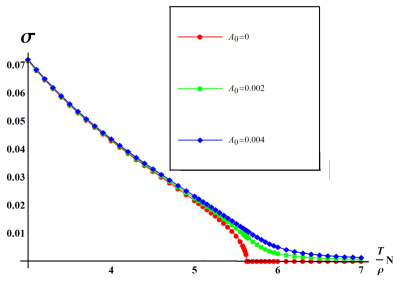
Figure 1: Plot of the nematic order parameter ($\sigma$) vs. temperature for different values of external field $A_{0}$ = 0 (red), 0.001 (green),0.01 (blue). The parameters chosen are $\rho\Lambda^{2}=1,g=0.3$ and $\rho_{z}=0.01$.

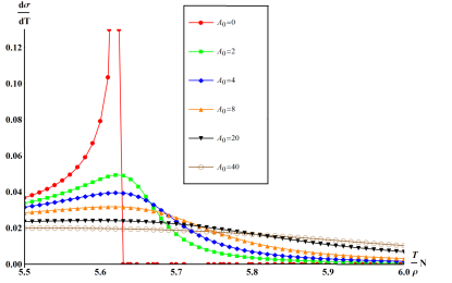
Figure 2: Plot of the derivative of the nematic order parameter vs. temperature for different external fields $A_{0}(10^{-3})$. The parameters used are $\rho_{z}=0.01,g=0.3,\rho=\Lambda=1$.

Taking $\lambda=\sigma_{a}+\rho_{z}/T$, we can derive the magnetic transition $T_{AF}$, which is determined by the following equations,

$$\frac{\sigma_{AF}}{g} = \frac{1}{8\pi\rho}ln\left[\frac{2\sigma_{AF}^{\prime}T_{AF}+{\rho_{z}}+2\sqrt{\left(\sigma_{AF}^{\prime}T_{AF}\right)^{2}+{\sigma_{AF}^{\prime}\rho_{z}}}}{\rho_{z}}\right]$$

$$\frac{\sigma_{AF}}{g} = \frac{1}{4\pi\rho}ln\frac{2\rho}{\rho_{z}}-\frac{1}{T_{AF}}$$

where $\sigma_{AF}^{\prime}=\sigma_{AF}+\frac{A_{0}}{T_{AF}}$. For $A_{0}=0$ and $\rho\Lambda^{2}>g>>\rho_{z}$, the magnetic transition temperature $T^{*}_{AF}$ is approximately

$$T^{*}_{AF}\approx T_{AF}^{0}+\frac{(T_{AF}^{0})^{2}}{8\pi\rho}\left[ln\frac{4g}{\rho_{z}}+ln\left(\frac{T_{AF}^{0}}{8\pi\rho}ln\frac{4g}{\rho_{z}}\right)\right]$$ (7)

where $T_{AF}^{0}=\frac{4\pi\rho}{ln\frac{2\rho}{\rho_{z}}}$. For small external strain field, $A_{0}<<g$, the shift in the magnetic ordering temperature, $\Delta T_{AF}=T_{AF}(A_{0})-T^{*}_{AF}$, to linear order is

$$\Delta T_{AF}=\frac{T^{*}_{AF}}{(8\pi\rho-T^{*}_{AF})\sigma_{AF}-g}A_{0}.$$ (8)

Since $\sigma_{AF}\sim g$, the coefficient in the right side of the above equation goes as $\sim 1/g$ for small $g$. The above results can be extended even in the limit of $g\to 0$. It is easy to show that in this limit, $T_{\cal N}-T_{AF}\sim g^{1/2}$. Plugging this into Eq.8, we obtain the expression below Eq. 3.

Eq. 3 can be further checked in the case of $g=0$. For $g=0$, the change of magnetic transition temperature is given by

$$\Delta T_{AF}=\frac{J_{z}}{4\pi\rho(\frac{J_{z}}{T_{AF}^{0}})^{3/2}}\sqrt{T_{AF}^{0}|A_{0}|}$$ (9)

consistent with the expectations of scaling theory, Eq. 3.

Comparison with experiment: Fig. 3 shows the comparison of our theoretical results with experimental observations of Dhital et al for the magnetic transition and nematic crossover as a function of uniaxial strain. The parameters used to generate the theoretical results, represented by the lines in the figure, are presented in the figure caption. The upper curve, representing the nematic crossover, is solid where there is a well-defined inflection point associated with the crossover, and a dashed line where the crossover has become so smooth that there is no local maximum in the temperature derivative of the nematic order parameter. The lower line indicates the theoretical magnetic ordering temperature. Fig. 4 shows the variation of the nematic transition with $A_{0}$ from which Fig. 3 was obtained. The close correspondence between the theoretical and experimental curves supports the conjecture that the starting model captures the essential physics, although the comparison involves too many empirically determined parameters to make this conclusion inescapable.

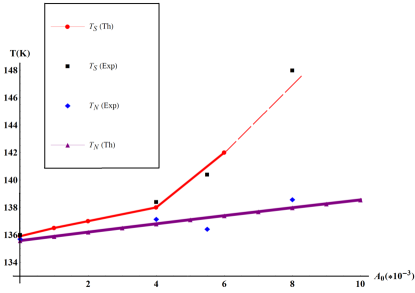
Figure 3: Comparison of the external field, $A_{0}$, variation of Magnetic Ordering Temperature and Nematic transition temperature with experiment.The parameters chosen are $\rho_{z}=0.06\rho,g=0.3\rho,\rho\sim 71K$.

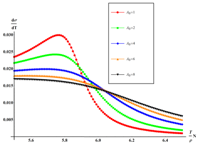
Figure 4: Variation of the Nematic order jump with external field $A_{0}$. The parameters chosen are the same as Fig. 3 with N=3 and $A_{0}$ in units of $10^{-3}$.

In order to match the experimental transition temperature, the value of $\rho$ used in our theoretical calculation ( see the caption of Fig. 3) is smaller than the value measured in neutron scattering experimentsZhao et al. (2009). This is expected since the transition temperature is always overestimated when $N$ is taken to be 3 in the large N expression.

In summary, we have shown that the minimal model with short ranged magnetic exchange couplings can satisfactorily account for the change of both structural and AF transition temperatures under the uniaxial stain measured by Dhital et al in $BaFe_{2}As_{2}$. The experimental results strongly support the notion of the magnetically-driven nematicity in iron-pnictides.

Acknowledgement: The work is supported in part by the Ministry of Science and Technology of China 973 program(2012CV821400) and NSFC-1190024, and by DOE grant # AC02-76SF00515 at Stanford (S. A. K.).

References

- (1) Dhital C, Z. Yamani, Wei Tian, J. Zeretsky, A. S. Sefat, Ziqiang Wang, R. J. Birgeneau and Stephen D. Wilson, arXiv:1111.2326 (2011).
- de la Cruz et al. (2008) C. de la Cruz, Q. Huang, J. W. Lynn, J. Li, W. R. II, J. L. Zarestky, H. A. Mook, G. F. Chen, J. L. Luo, N. L. Wang, et al., Nature 453, 899 (2008).
- Zhao et al. (2008a) J. Zhao, Q. Huang, C. de la Cruz, S. Li, J. W. Lynn, Y. Chen, M. A. Green, G. F. Chen, G. Li, Z. Li, et al., Nature Materials 7, 953 (2008a).
- (4) In fact, the symmetry involved is typically not a simple rotation, but rather a rotation followed by reflection through the Fe plane - this subtlety does not affect the following discussion.
- Fang et al. (2008a) C. Fang, H. Yao, W.-F. Tsai, J. Hu, and S. A. Kivelson, Phys. Rev. B 77, 224509 (2008a).
- Xu et al. (2008) C. Xu, M. Mueller, and S. Sachdev, Phys. Rev. B 78, 20501 (2008).
- (7) Jiangping Hu and Cenke Xu, arXiv:1112.2713 (2011).
- Fradkin et al. (2010) E. Fradkin, S. A. Kivelson, M. J. Lawler, J. P. Eisenstein, and A. P. Mackenzie, Annual Review of Condensed Matter Physics 1, 153 (2010).
- Fisher et al. (2011) I. R. Fisher, L. Degiorgi, and Z. X. Shen, Reports on Progress in Physics 74, 124506 (2011).
- Ying et al. (2011) J. J. Ying, X. F. Wang, T. Wu, Z. J. Xiang, R. H. Liu, Y. J. Yan, A. F. Wang, M. Zhang, G. J. Ye, P. Cheng, et al., Physical Review Letters 107, 067001 (2011).
- Chuang et al. (2010) T.-M. Chuang, M. P. Allan, J. Lee, Y. Xie, N. Ni, S. L. Bud’ko, G. S. Boebinger, P. C. Canfield, and J. C. Davis, Science 327, 181 (2010).
- Zhao et al. (2009) J. Zhao, D. T. Adroja, D. X. Yao, R. Bewley, S. L. Li, X. F. Wang, G. Wu, X. H. Chen, J. P. Hu, and P. C. Dai, Nature Physics 5, 555 (2009).
- Harriger et al. (2010) L. W. Harriger, H. Luo, M. Liu, T. G. Perring, C. Frost, J. Hu, M. R. Norman, and P. Dai, Phys. Rev B 84, 054544 (2010).
- Nakajima et al. (2011) M. Nakajima, T. Liang, S. Ishida, Y. Tomioka, K. Kihou, C. H. Lee, A. Iyo, H. Eisaki, T. Kakeshita, T. Ito, et al., PNAS 108, 12238 (2011).
- Yi et al. (2011a) M. Yi, D. H. Lu, J.-H. Chu, J. G. Analytis, A. P. Sorini, A. F. Kemper, S.-K. Mo, R. G. Moore, M. Hashimoto, W. S. Lee, et al., ArXiv:1011.0050 (2011a).
- Yi et al. (2011b) M. Yi, D. H. Lu, R. G. Moore, K. Kihou, C.-H. Lee, A. Iyo, H. Eisaki, T. Yoshida, A. Fujimori, and Z.-X. Shen, Arxiv:1111.6134 (2011b).
- (17) R. M. Fernandes, E. Abrahams, and J. Schmalian, Phys. Rev. Lett. 107, 217002 (2011) and R.M. Fernandes, A. V. Chubukov, J. Knolle, I. Ermin, and J. Schmalian, arXiv:1110.1893 (2011).
- Wysocki et al. (2011) A. L. Wysocki, K. D. Belashchenko, and V. P. Antropov, Nature Physics 7, 485 (2011).
- Hu et al. (2011) J. Hu, B. Xu, W. Liu, N. Hao, and Y. Wang, ArXiv:1106.5169 (2011).
- (20) So long as is not too large, the large approach can be straightforwardly extended to include the effects of non-zero , but it has little effect on the results.
- (21) Under some circumstances, there could be a metanematic transition, even for , but this does not seem to occur in the limit.