Detection of a small shift in a broad distribution

Abstract

Statistical methods for the extraction of a small shift in broad data distributions are examined by means of Monte Carlo simulations. This work was originally motivated by the CERN neutrino beam to Gran Sasso (CNGS) experiment for which the OPERA detector collaboration reported a time shift in a broad distribution with an accuracy of $\pm 7.8\,$ns, while the fluctuation of the average time turns with $\pm 23.8\,$ns out to be much larger. Although the physical result of a big shift has been withdrawn, statistical methods that make an identification in a broad distribution with such a small error possible remain of interest.

1 Introduction

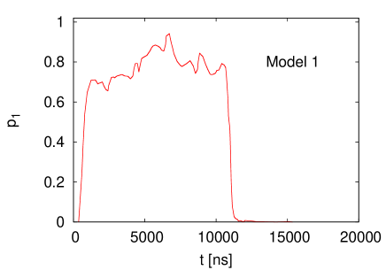
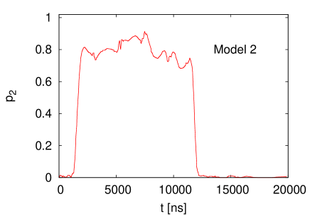
Figure 1: Departure time probability densities modeled after Fig. 11 of Ref. [1].

In highly publicized CERN announcements [1] it was claimed that neutrinos from the CNGS arrived at Gran Sasso

$$\delta t=\rm\left[-57.8\pm 7.8\ (stat.)\,\matrix{+8.3\cr-5.9}\ (sys.)\right]\,ns$$ (1)

too early, violating the $\delta t=0$ limit set by the speed of light. Meanwhile, initially overlooked systematic errors [2] have wiped out the estimate of a large shift. But the estimate of the statistical error remains of interest as it exemplifies the extraction of a small shift from a broad distribution. The purpose of this article is to shed light on subtleties of an analysis, which leads to the statistical part of the estimate (1).

The CNGS sample of $15\,223$ neutrinos was produced in extractions that last about 10,500 ns each. Two different types of extractions were used leading to probability densities (PD)

$$p_{k}(t)\,,~{}~{}k=1,2$$ (2)

for neutrinos departure times, which are reproduced here in Fig. 1. The PD used in our paper have been discretized in intervals of 1 ns and can be downloaded from the author’s website [3].

One can now perform a statistical bootstrap [4] analysis by Monte Carlo (MC) generation of departure times with the PD of Fig. 1. This is already remarked in [1], where the application remains limited to testing of their maximum likelihood procedure on a sample of 100 MC data sets. As the MC generation of departure times can be repeated almost arbitrarily often with distinct random numbers, one can analyze and verify statistical methods that one wants to apply to discover a shift in the data.

For the uniform PD over 10 500 ns, it has been noted [5] that with $n=16\,111$ events the variance of the departure time average $\overline{t}$ is approximately $\triangle\overline{t}=24\,$ns, i.e., much larger than the statistical error bar in Eq. (1). It will be discussed in this paper that the time shift $\delta t$ (1) defined in [1] behaves indeed differently than a statistical fluctuation of the time average

$$\delta\overline{t}=\frac{n_{1}\,\delta\overline{t}_{1}+n_{2}\,\delta\overline{t}_{2}}{n_{1}+n_{2}}\,,~{}~{}\delta\overline{t}_{i}=\overline{t}_{i}-\widehat{t}_{i}\,,~{}~{}i=1,\,2\,.$$ (3)

Here $\overline{t}_{i}$ are the measured departure time averages, $\widehat{t}_{i}$ are the mean departure times obtained from the underlying PD, and $n_{i}$ are the numbers of events in each extraction. The distinction between $\delta t$ (1) and $\delta\overline{t}$ (3) is made by an overline on $t$ or not. Obviously,

$$\langle\delta t\rangle\ =\ \langle\delta\overline{t}\rangle$$ (4)

holds for the expectation values, but their error bars behave differently.

To set the groundwork, it is shown in section 2 for the uniform distribution that a shift $\delta t=-57.8\,$ns can be identified with certainty (probability to miss it $<10^{-36}$) when there are 15 223 events and the departure time range is $10\,500\,$ns. In section 3 the MC generation of departure times is described. Section 4 gives examples of descriptive histograms from MC data. Suggested by the uniform distribution, the front tails of the distributions are of particular interest. For their study the cumulative distribution function (CDF) is better suited than a histogram, because it allows easily to focus on outliers. This is investigated in section 5. To estimate the shift value $\delta t$, the maximum likelihood method is used in [1]. In section 6 features of this method are calculated by applying it to a large number of MC generated departure time samples.

Independently of the special example, the approaches discussed in sections 2 to 6 are of interest, because they address the general problem of extracting a precise estimate of a shift from a broad distribution. Summary and conclusions follow in section 7.

2 Uniform Distribution

Using the uniform PD over a time window of 10 500 ns, the standard deviation of the average

$$\overline{t}\ =\ \frac{1}{n}\sum_{j=1}^{n}t^{j}$$ (5)

is for $n=15\,223$ events much larger than the statistical error bar quoted in Eq. (1), namely approximately

$$\triangle\overline{t}\ =\ 25\,{\rm ns}\,.$$ (6)

How can this be? That the average (5) fluctuates with the variance (6) is unavoidable. However, the effect we are after is a systematic shift of each departure time by an amount $\delta t=-57.8\,$ns. Again for the uniform uniform distribution, drawn in Fig. 2, it is easily illustrated that this can very well be identified. Events indicated on the left of the figure are impossible unless there is a shift. Now, with a shift of $-57.8\,$ns the probability to find a particular event to the left of the uniform PD is given by

$$p\ =\ 57.8/10\,500\ =\ 0.005505\dots$$ (7)

and the probability to find none is

$$(1-p)^{15\,672}\ =\ 10^{-36.5}\,.$$ (8)

The distance of the smallest time from the left edge of the uniform PD is a lower bound on $\delta t$ and a direct estimate for the time shift (1) is

$$\delta t=n_{\rm left}\,10\,500\,{\rm ns}\,/\,15\,223\,,$$ (9)

where $n_{\rm left}$ is the number of events observed on the left outside of the uniform PD. Confidence limits can be established from the binomial distribution.

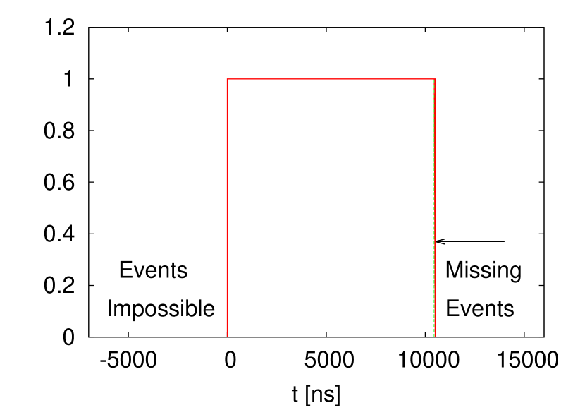
Figure 2: Uniform distribution: Impossible (left) and missing events (in the enlarged thickness of the right border).

For the tiny range of $57.8\,$ns indicated by the somewhat thicker line on the right side of the uniform PD in Fig. 2, the situation is the other way round. It has to be empty when there is a shift by $\delta t=-57.8\,$ns. The probability that this happens by chance when there is in fact no shift is also given by (9). When $\delta t$ is not known the distance of the largest measured time from the right edge of the uniform PD is an upper bound on $\delta t$.

We do not pursue the uniform PD any further, because we are interested in the more complicated case of the less sharp PD of Fig. 1.

Figure 3: Enlargement of the approximated PD for model 1 over a small time region.

3 MC generation of departure times

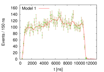
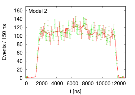
Figure 4: Typical histograms of departure times together with the PD of Fig. 1. For the (online) green entries the generated time distribution is shifted by 57.8 ns to the left.

As mentioned in the introduction, the PD of Fig. 1 have been discretized in 1 ns intervals and are available on the Web [3]. The resolution of 1 ns allows for easy MC generation of departure times and is sufficient for the intended accuracy of the estimate of a shift. In the following our thus defined models are labeled by $k=1,2$. The probabilities as function of time $t$ are defined by

$$p_{k}(t)\ =\ p_{k}(i^{t})~{}~{}{\rm for}~{}~{}i^{t}\leq t<i^{t}+1\,,$$ (10)

where $i^{t}$ are integers in ns units. As it is convenient for the MC generation of departure times, the normalization for the discretized PD is (distinct from Fig. 1) chosen so that

$$p^{\max}_{k}\ =\ \max_{i}\left[p_{k}(i)\right]\ =\ 1$$ (11)

holds. Proper normalizations $\sum_{i}p_{k}(i)\,\triangle t_{k}=1$ could still be achieved by choosing instead of ns some unconventional unit for $\triangle t_{k}$. For the generation of correctly distributed random times this is irrelevant. For a short time range model 1 probabilities $p_{1}(t)$ are enlarged in Fig. 3.

After discretization the smallest $i^{\min}_{k}$ and largest $i^{\max}_{k}$ times with non-zero $p_{k}(i^{t})$ values are

$$i^{\min}_{1} = 359~{}~{}~{}{\rm and}~{}~{}~{}i^{\max}_{1}\ =\ 15\,368\,,$$

$$i^{\min}_{2} = ~{}\,12~{}~{}~{}{\rm and}~{}~{}~{}i^{\max}_{2}\ =\ 19\,877\,.$$

In particular for the large $i^{t}$ values, these ranges include a number of zero probabilities. MC generated departure times $t_{k}^{j}$ ($j=1,\dots,n$) with $n$ the number of data are obtained from uniformly distributed random numbers $t$ in a range enclosing $\left(i^{\min}_{k},i^{\max}_{k}+1\right)$, here chosen to be (1,22000): for model $k$ a proposed random time $t$ is accepted with probability $p_{k}(i^{t})$ for $i^{t}\leq t<i^{t}+1$. If $t$ is rejected, the procedure is repeated until a value gets accepted, which then becomes a data point $t_{k}^{j}$. Acceptance rates were close to 40% and the random number generator of Ref. [6] has been used. To avoid direct hits of $i^{\min}_{k}$ and associated rounding problems, the proposed random times are shifted by $+2^{-25}$, which is half the discretization [7] of these random numbers.

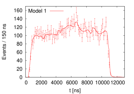
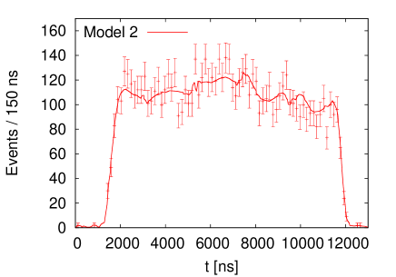
Figure 5: Histograms of departure times with a combined average fluctuation of $\delta\overline{t}=-59.6\,$ns.

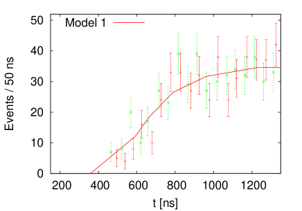
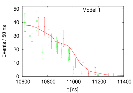
Figure 6: Model 1: Zoom of the leading (left plot) and trailing (right plot) MC generated departure time histograms from Fig. 5 (red online) with the PD and plotted together with Fig. 4 histograms shifted by $\delta t=-57.8\,$ns (green online).

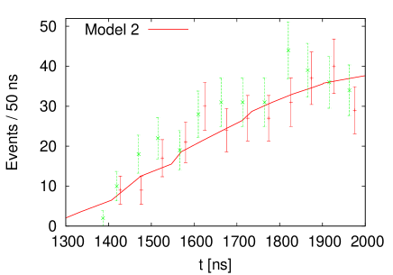
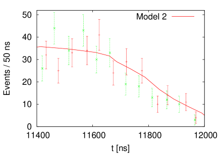
Figure 7: Model 2: Zoom of the leading (left plot) and trailing (right plot) MC generated departure time histograms from Fig. 5 (red online) with the PD and plotted together with Fig. 4 histograms shifted by $\delta t=-57.8\,$ns (green online).

4 Histograms

In this section we pursue descriptive statistics and show histograms from samples of $n=7\,612$ MC generated departure times per model. The exact departure time mean values for our discretized PD of Fig. 1 are (the hat indicates exact):

$$\hat{t}_{1}=\langle t\rangle_{1}=5942.2\,{\rm ns}\,,\ \hat{t}_{2}=\langle t\rangle_{2}=6658.7\,{\rm ns}\,,$$ (12)

where model 1 and 2 are again labeled by the corresponding subscripts. We also know from these PD the exact standard deviations for time averages $\overline{t}_{1}$ and $\overline{t}_{2}$, each over $n=7\,612$ events:

$$\widehat{\triangle}\overline{t}_{1}\ =\ 33.4\,{\rm ns}\,,~{}~{}~{}\widehat{\triangle}\overline{t}_{2}\ =\ 33.8\,{\rm ns}\,.$$ (13)

Their combined standard deviation is

$$\widehat{\triangle}\overline{t}\ =\ 23.8\,{\rm ns}\,,$$ (14)

which agrees almost with the estimate (6) from the uniform PD.

Together with the PD, Fig. 4 shows (red online) histograms of 150 ns bin width for departure times from a typical [8] MC generated sample of 7 612 events per model and again the same histograms (green online) shifted by $-57.8\,$ns. This illustrates how small the effect is, which has to be unambiguously identified.

Rounded to nearest integers the mean values for the time averages of the data of Fig. 4 are

$$\overline{t}_{1} = (5936\pm 34)\,{\rm ns~{}~{}(model~{}1)}\,,$$ (15)

$$\overline{t}_{2} = (6703\pm 34)\,{\rm ns~{}~{}(model~{}2)}\,.$$ (16)

Both are within statistical uncertainties consistent with the mean values (12) of the PD. The actual statistical fluctuations of these two MC data sets are (using $\overline{t}_{1}=5935.5$ and $\overline{t}_{2}=6703.2$)

$$\delta\overline{t}_{1} = \overline{t}_{1}-\hat{t}_{1}\ =\ -6.7\,{\rm ns}\,,$$ (17)

$$\delta\overline{t}_{2} = \overline{t}_{2}-\hat{t}_{2}\ =\ 44.5\,{\rm ns}\,,$$ (18)

with an average of 18.9 ns.

To compare the shift of $\delta t=-57.8\,$ns with a statistical fluctuation of at least the same size, the MC generation was repeated one million times and in this process 7 608 samples (0.76%) with statistical fluctuations $\delta\overline{t}\leq-57.8\,$ns were encountered. The PD of the first of these MC samples are shown in Fig. 5. They feature the time averages

$$\overline{t}_{1} = (5907\pm 34)\,{\rm ns,~{}~{}(model~{}1)}\,,$$ (19)

$$\overline{t}_{2} = (6575\pm 34)\,{\rm ns,~{}~{}(model~{}2)}\,,$$ (20)

with the actual statistical fluctuations (using $\overline{t}_{1}=5906.7$ and $\overline{t}_{2}=6575.0$)

$$\delta\overline{t}_{1} = \overline{t}_{1}-\hat{t}_{1}\ =\ -35.5\,{\rm ns}\,,$$ (21)

$$\delta\overline{t}_{2} = \overline{t}_{2}-\hat{t}_{2}\ =\ -83.7\,{\rm ns}\,,$$ (22)

resulting in an average of $-59.6\,$ns.

Figures 6 and 7 zoom into the leading and trailing parts of the departure times of Fig. 5 (red online) and compare them with the shift by $-57.8$ of Fig. 4 (green online). The binsize is from $150\,$ns reduced to $50\,$ns, so that it is now slightly smaller than the shift, while the noise in the histogram increases. By visual inspection of histograms it is difficult to distinguish a shift of all times from a statistical fluctuation. The analysis of the uniform distribution in section 2 suggests to display the tails of the distribution event by event. Using the empirical CDF this is done next.

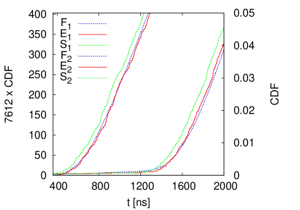
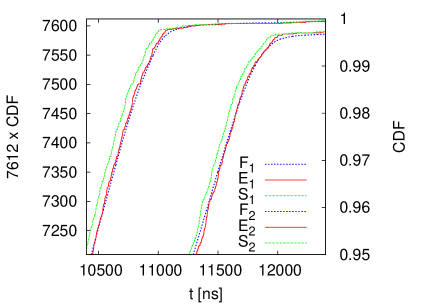
Figure 8: Tails of the CDF ($F_{k}$ exact, $E_{k}$ empirical, $S_{k}$ empirical shifted by $-57.8\,$ns, $k=1,2$ models).

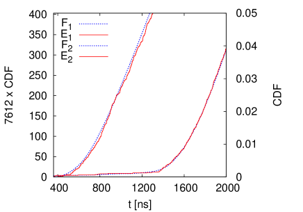
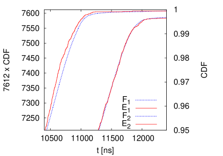
Figure 9: Tails of the CDF for departure times with a $-59.6\,$ns statistical fluctuation ($F_{k}$ exact, $E_{k}$ empirical).

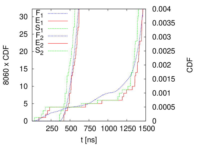
Figure 10: Enlargement of the left part of Fig. 8.

5 Cumulative distribution functions (CDF)

For continuous distributions a problem of histograms is that a binsize needs to be chosen. In our case we need a good resolution on the time axis, i.e., a small binsize. However, this increases the noise of the bin average. As the empirical CDF has no such free parameter, it is better suited for the analysis at hand. In particular, it is well suited for a display of the tails of a distribution. Based on the binomial distribution we will develop their quantitative analysis relying on uniformly distributed random variables, similarly as for the goodness of fit [7].

The exact CDF of our PD models are

$$F_{k}(t)\ =\ \int_{-\infty}^{t}dt^{\prime}\,p_{k}(t^{\prime})\,,~{}~{}k=1,2\,,$$ (23)

where $p_{k}(t)$ is given by (10). The empirical CDF $E_{k}(t)$ are calculated from the data (see, e.g., [7]), which are here MC generated random times. Let them be $t^{1}_{k},\dots,t^{n}_{k}$ and $t^{\pi_{1}}_{k},\dots,t^{\pi_{n}}_{k}$ sorted, so that $t^{\pi_{i}}_{k}<t^{\pi_{i+1}}_{k}$ holds for $i=0,\dots,n+1$, where the definitions $t_{k}^{\pi_{0}}=-\infty$ and $t_{k}^{\pi_{n+1}}=+\infty$ have been added. The empirical CDF are then defined by

$$E_{k}(t) = {i\over n}~{}~{}~{}{\rm for}~{}~{}~{}t^{\pi_{i}}_{k}\leq t<t^{\pi_{i+1}}_{k},$$ (24)

$$i = 0,1,\dots,n,n+1\,.$$

Shifted by $\delta t$ the empirical CDF are

$$S_{k}(t)\ =\ E_{k}(t-\delta t)\,.$$ (25)

For the data sets of random times used in the previous section $F_{k}(t)$, $E_{k}(t)$ and $S_{k}(t)$ with $\delta t=-57.8\,$ns are displayed in Fig. 8. The scale on the right ordinates gives the usual probability definition for which a CDF is in the range $[0,1]$, while the scale on the left ordinates is chosen to count the number of included data points. Fig. 8 should be compared with Fig. 9, which features the statistical fluctuation (21), (22) of the average time by $-59.6\,$ns. While the $-57.8\,$ns shift is clearly visible for all four cases of Fig. 8, there is ony in one case a similar signal in Fig. 9.

In the figures on the right side $F_{k}(t)=1$ is only slowly approached, because in the PD there are small contributions from the region starting between $15\,000\,$ns and $20\,000\,$ns (about 30 events for model 2 for which the effect is larger than for model 1). This does not spoil the over-all picture, so that the accuracy of the PD in this region does not really matter.

Visually, shift and statistical fluctuation behave already differently, though not always. The task is now to develop quantitative criteria, which are in this section based on the binomial distribution. Defining

$$F^{i}_{k}\ =\ F_{k}(t^{\pi_{i}}_{k})~{}~{}{\rm and}~{}~{}G^{i}_{k}=1-F^{i}_{k}$$ (26)

the probability for a single data point $t$ to be in the range $0\leq F_{k}(t)\leq F^{i}_{k}$ is $F^{i}_{k}$ and its probability to be in the range $F^{i}_{k}<F_{k}(t)\leq 1$ is $G^{i}_{k}$. The probability that $i$ out of $n$ data points are in the $0\leq F_{k}(t)\leq F^{i}_{k}$ range is

$$p^{i}_{k}\ =\ \frac{n!}{(n-i)!\,i!}\,\left(F^{i}_{k}\right)^{i}\,\left(G^{i}_{k}\right)^{n-i}\,.$$ (27)

If there is a shift by $\delta t<0$ we expect that more data points populate the $0\leq F_{k}(t)\leq F^{i}_{k}$ range, so that

$$Q^{i}_{k}\ =\ \sum_{j=i}^{n}p^{j}_{k}$$ (28)

becomes small. It is easy to see that the $Q^{i}_{k}$ are uniformly distributed random variables, when the hypothesis is correct that the data points are created with the distribution $F_{k}(t)$. So the usual interpretation [7] of a likelihood that the discrepancy between the hypothesis and the data is due to chance applies to the $Q^{i}_{k}$.

To present an example we give in Fig. 10 an enlargement of the left tail from Fig. 8 by picking out the 32 smallest times per model. Upon inspection of the numbers one finds for model 1 $t_{1}^{\pi_{1}}=359.985\,$ns and $F^{1}_{1}=F_{1}(t_{1}^{\pi_{1}})=5.7\times 10^{-9}$. This implies $Q^{1}_{1}=4.3\times 10^{-5}$ for model 1. For model 2 $t^{\pi_{1}}_{2}=29.968\,$ns, which gives $F^{1}_{2}=F_{2}(t_{2}^{\pi_{1}})=3.5\times 10^{-6}$ and for $n=7612$ one finds $Q^{1}_{2}=0.026$. Combined, these two events alone give a probability $Q=Q^{1}_{1}\,Q^{1}_{2}=1.15\times 10^{-6}$ for the likelihood that the discrepancy is due to chance.

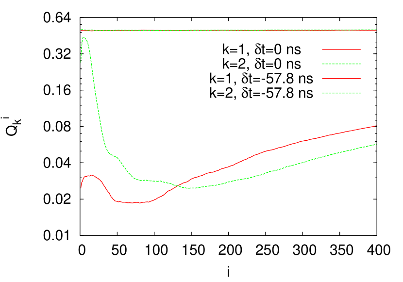
Figure 11: Average $Q^{i}_{k}$ as functions of $i$ from $10\,000$ samples.

To understand the typical behavior encountered for our two distribution functions, we generated $10\,000$ MC samples. In Fig. 11 average values for $Q^{i}_{k}$ are shown using a log scale on the ordinate. The almost straight lines at 0.5 are the averages obtained when one generates random times with the underlying PD. The two other lines correspond to the average $Q^{i}_{k}$ obtained when each sample undergoes a shift of $-57.8\,$ns. For increasing $i$ (out of the range of the figure) they will approach 0.5, because the shift has little effect in the middle of a broad distribution.

At a first glance the average $Q^{1}_{k}$ values for the smallest times look far less promising than what we may have hoped for from the inspection of our trial sample. For model 1 the average is at 0.025 and for model 2 even at 0.27. At a second look we shall see that this comes mainly from the outliers of the non-Gaussian distribution of the $Q^{1}_{k}$, while for a majority of cases our trial sample remains typical. Besides $Q^{1}_{k}$ for the smallest times, an attractive choice for $Q^{i}_{k}$ is at or close to the minimum of the average, which we choose to be $i=80$ for model 1 and $i=160$ for model 2. Due to the increased number of data there are fewer outliers than for $Q^{1}_{k}$. Note that for different $i$ values the $Q^{i}_{k}$ are not statistically independent, because the calculation of $Q^{i}_{k}$ includes all data already used for $Q^{j}_{k}$ with $j<i$.

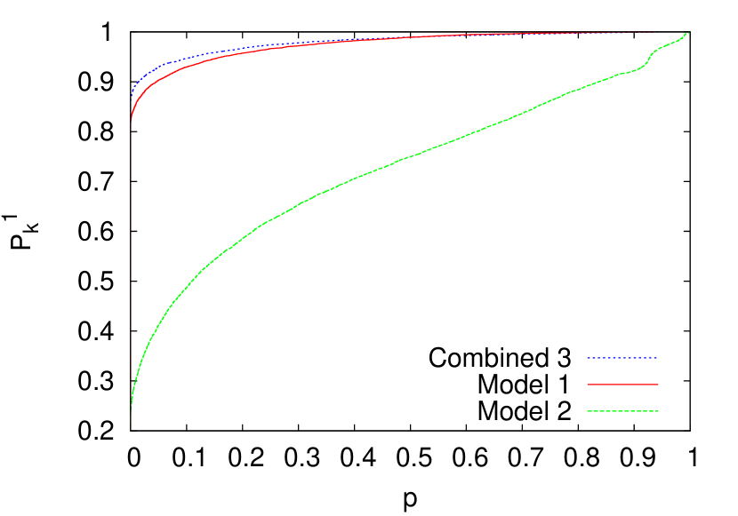
Figure 12: Probabilities $P^{1}_{k}$ for $Q^{1}_{k}\leq p$, $\delta t=-57.8\,$ns, from 10 000 samples.

We define $P^{i}_{k}(p)$ to be the probability for $Q^{i}_{k}\leq p$. Fig. 12 plots $P^{1}_{k}(p)$ and we find $Q^{1}_{1}=0$ for more than 80% of the samples and $Q^{1}_{2}=0$ for almost 23% of the samples. To combine the results from both models we notice that

$$Q^{ij}_{3}\ =\ Q^{i}_{1}\,Q^{j}_{2}\,\left[1-\ln(Q^{i}_{1}\,Q^{j}_{2})\right]$$ (29)

is again a uniformly distributed random variable with the interpretation that the discrepancy between data and hypothesis is due to chance ($Q^{ij}_{3}\to Q^{i}_{1}Q^{j}_{2}$ for $Q^{i}_{1}$ or $Q^{j}_{2}$ to zero). We use the notation $Q^{i}_{3}=Q^{ii}_{3}$ and find $Q^{1}_{3}=0$ for more than 85% of the samples, where (29) is of course performed before sorting.

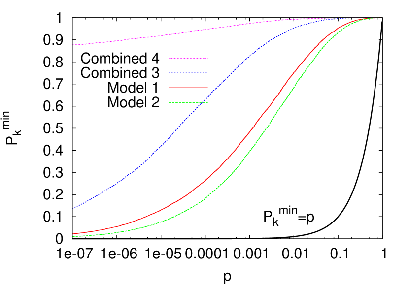
Figure 13: Probabilities $P^{\min}_{k}$ for $Q^{\min}_{k}\leq p$, $\delta t=-57.8\,$ns, from 10 000 samples (log scale on the abscissa).

We define now $Q^{\min}_{1}=Q^{80}_{1}$, $Q^{\min}_{2}=Q^{160}_{2}$ and $Q^{\min}_{3}$ the combination (29) of the two. $P^{\min}_{k}(p)$ are the corresponding probabilities for $Q^{\min}_{k}\leq p$. In Fig. 13 the $P^{\min}_{k}(p)$ are plotted versus $p$ using a log scale on the abscissa (the line $P^{\min}_{k}=p$ is no longer straight). The $Q^{\min}_{k}$ probabilities tend to be small, but never zero. For the combined data we find $Q^{\min}_{3}\leq 10^{-7}$ for about 14% and $Q^{\min}_{3}\leq 10^{-3}$ for more than 82% of the samples. Now $Q^{\min}_{3}$ works quite independently from $Q^{1}_{k}$, reducing the situations, where their combined estimate $Q^{\min}_{4}=Q^{\min}_{3}\,Q^{1}_{3}\,\left[1-\ln(Q^{\min}_{3}\,Q^{1}_{3})\right]$ gives $Q^{\min}_{4}>10^{-3}$ to approximately 2.6%. Compare Fig. 13. Although the application of Eq. (29) is not entirely correct for $Q^{\min}_{4}$, the related bias is small as it comes from the contribution of single data points $t^{\pi_{1}}_{k}$ to each of the $Q^{\min}_{k}$.

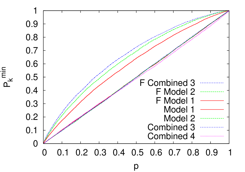
Figure 14: Diagonal lines: Probabilities $P^{\min}_{k}$ for $Q^{\min}_{k}\leq p$, $\delta t=0\,$ns. Upper curves (F): The same with a statistical fluctuation $\delta\overline{t}\leq-57.8\,$ns of each sample average. Each curve relies on 10 000 samples.

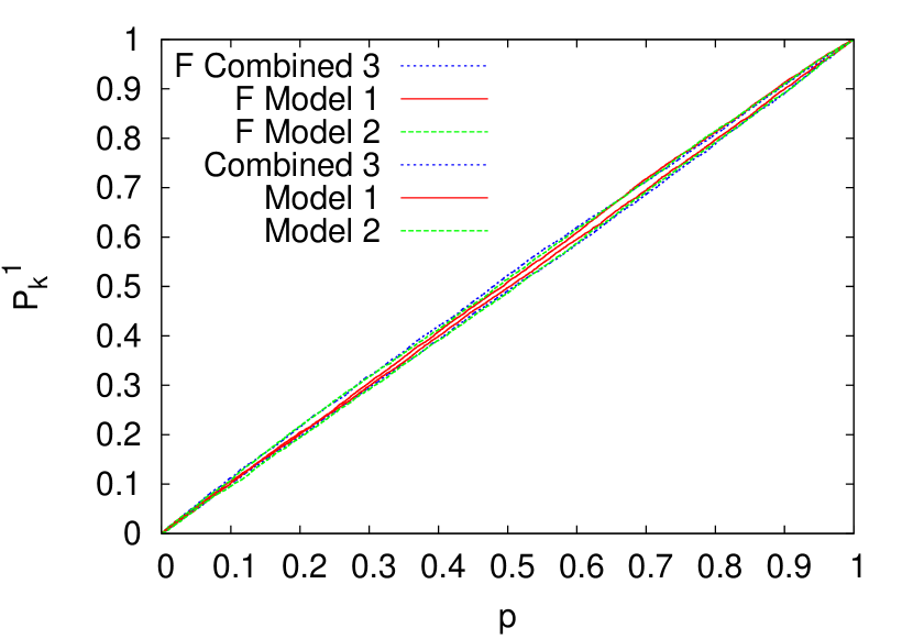
Figure 15: Probabilities $P^{1}_{k}$ for $Q^{1}_{k}\leq p$, $\delta t=0\,$ns and (F) the same with a statistical fluctuation $\delta\overline{t}\leq-57.8\,$ns of each sample average. Each curve relies on 10 000 samples.

For the peace of mind we show in Fig. 14 the $P^{\min}_{k}$ values when no shift is applied to the data. As claimed the $Q^{\min}_{k}$ turn out to be uniformly distributed random variables in the $[0,1)$ range with a small bias visible for $Q^{\min}_{4}$. These are the almost straight $P^{\min}_{k}(p)=p$ lines. The upper part of the figure shows $P^{\min}_{k}(p)$ from $10\,000$ samples, which are selected so that each exhibits a statistical fluctuation $\delta\overline{t}\leq-57.8\,$ns (as about 0.76% of the samples exhibit such a fluctuation it requires the generation of more than 13 million samples). In contrast to Fig. 13 the $P^{\min}_{k}(p)$ probabilities for $Q^{\min}_{k}\leq p$ are only slightly enhanced when compared to the straight line. The same analysis shows for $Q^{1}_{k}$ practically no deviation from the straight $P^{1}_{k}(p)=p$ lines as is demonstrated in Fig. 15. These statements remain true when a bias which enhances the initial tail of the PD (discussed in [5]) contributes to the shift in the mean value $\delta\overline{t}$.

In summary, there is high probability that a study of the initial tails of the departure time distributions reveals whether there is a statistically relevant shift or not. A similar study could be performed for the back tail of the departure times. One could further expand the analysis of this section to provide an explicit estimate of the shift $\delta t$, similarly as with Eq. (9) for the uniform PD, but now by bootstap simulation. Here we leave such an estimate to using the maximum likelihood method of the next section.

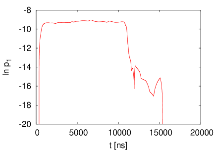
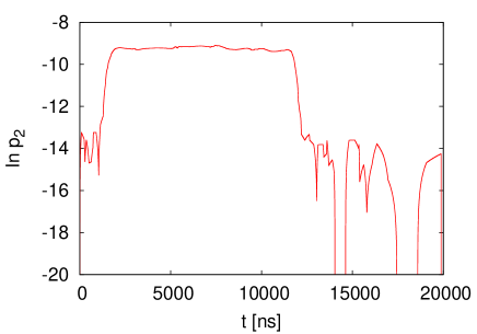
Figure 16: Departure time probability densities of Fig. 1 on a log scale.

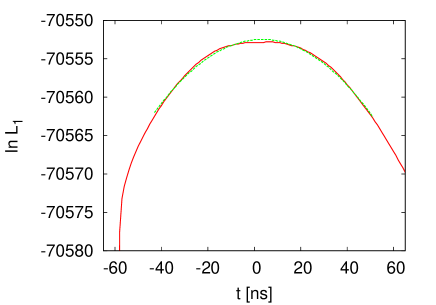
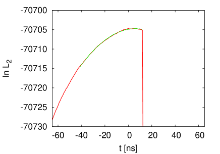
Figure 17: Log-likelihood functions (red online) of our typical sample for model 1 and 2. Parabolic fits (green online) are indicated for the central regions.

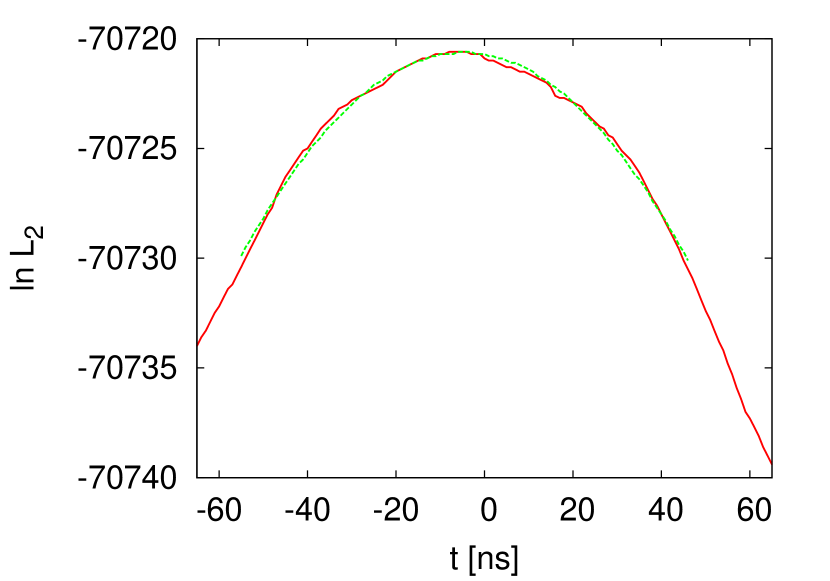
Figure 18: Log-likelihood function (red online) for model 2 from one of our first ten samples. A parabolic fit (green online) is indicated for the central region.

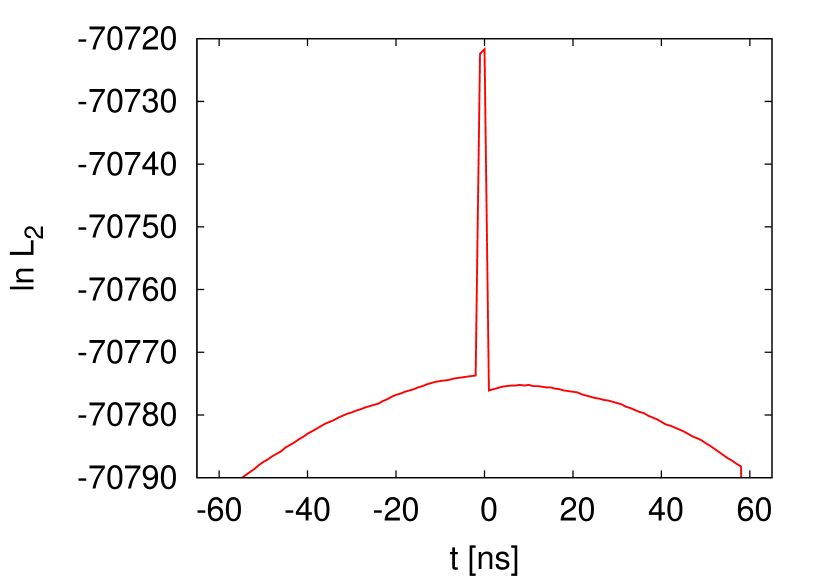
Figure 19: Log-likelihood function (red online) for model 2 from a sample for which a parabolic fit does not work.

6 Maximum likelihood method

For the statistical estimate of the time shift value $\delta t$ a maximum likelihood method is the choice of Ref. [1]. Its properties are studied in this section using $n=10\,$000 MC generated samples for each of the PD.

The log likelihoods for our PD (2) are given by

$$\ln L_{k}(t)\ =\ \sum_{i=1}^{n}\ln\left[p_{k}(t^{i}+t)\right],\ k=1,2$$ (30)

where the times $t^{i}$ are MC generated with the PD $p_{k}(t)$. It is instructive to replot Fig. 1 for logarithms of the probabilities. This is done in Fig. 16 with $p_{k}(t)$ normalized to $\sum_{i}p_{k}(t^{i})=1$, where (in accordance with our discretization) $t^{i}$ is incremented in 1 ns steps. These plots exhibit clearly the locations of small and zero probabilities, which data will (statistically) avoid when they are created with the underlying PD $p_{k}(t)$. However, when shifting the $t^{i}$ values in Eq. (30) by $t$, regions of low probabilities may be hit as discussed in the previous sections.

Our samples are generated without a shift $\delta_{\rm shift}t$, because the only effect of adding it would be that all $\delta t$ reported in this section become transformed according to

$$\delta t\ \to\ \delta t+\delta_{\rm shift}t\,.$$ (31)

Consequently, the $\delta t$ discussed in this section deal with the various error sources.

For our typical sample (see section 4) [8], the resulting $\ln L_{k}(t)$ functions are displayed in Fig. 17. For model 1 we see for decreasing $t$, just before $-60\,$ns, a sharp drop $\ln L_{1}(t)\to-\infty$. This comes because the smallest time, $t^{\pi_{1}}+t$ hits a tiny probability, which we already encountered in the previous section. For model 2 the log-likelihood function $\ln L_{2}(t)$ is smooth down to $t=-65\,$ns, while for positive $t>12\,$ns the largest data point $t^{\pi_{n}}+t$ hits a region of very small probability.

Fig. 18 shows for model 2 another log-likelihood function, $\ln L_{2}(t)$, from our first ten samples and this plot is quite similar to the one for extraction 2 in [1]. In the samples one finds a variety of deviations from Gaussian shapes, small ones due to the bulk structure of the PD and large ones due to a few events in the tails.

Following [1] a step further, parabolic fits are made to the central region of each sample. To automatize the fitting procedure the central region of a sample was defined to be the $t$ range connected with $\delta t_{k}$ so that $\ln L_{k}(t)>\ln L^{\max}_{k}-10$ holds, where the maximum of the log-likelihood function is

$$\ln L^{\max}_{k}=\max_{t}\left[\ln L_{k}(t)\right]=\ln L_{k}(\delta t_{k})\ .$$ (32)

Such parabolic fits are included in Fig. 17 and 18.

Let us investigate $\delta t_{k}$ estimates for random times generated with the PD (10). In the limit of infinite statistics

$$\lim_{n\to\infty}\frac{1}{n}\,\ln L_{k}(t)=\sum_{i}p_{k}(i)\,\ln p_{k}(i+t)$$ (33)

holds, where the sums corresponds to our discretization time steps of 1 ns. They include $p_{k}(i)=0$ contributions. For $t=0$ they are zero due to

$$\lim_{p\to 0}\left(p\,\ln p\right)\ =\ 0\,.$$ (34)

For $t\neq 0$, e.g. already $t=\pm 1\,$ns, we can create mismatched contributions $p_{k}(i)\ln p_{k}(t+t)$ with $p=p(i)$ finite and $q=p(i+t)=0$, so that

$$\lim_{q\to 0}\left(p\,\ln q\right)\ =\ -\infty$$ (35)

becomes possible. Hence, in the limit of infinite statistics

$$\lim_{n\to\infty}\left\langle\delta t_{k}\right\rangle_{n}\ =\ 0\ =\ \lim_{n\to\infty}\left\langle\left(\delta t_{k}\right)^{2}\right\rangle_{n}\,,$$ (36)

where $\langle\dots\rangle_{n}$ are expectation values for samples of $n$ data per model. Deviations of $\delta t_{k}$ from zero reflect statistical fluctuations and bias due to a finite statistics. In the following we investigate this for $n=7\,612$.

Direct estimates of $\delta t_{k}$ are obtained by simply evaluating the log-likelihood functions (30) for a sufficiently large region around its maximum, which is here taken to be [$-65\,$ns,$65\,$ns]. The positions of the maxima of the parabolic fits give also estimates of $\delta t_{k}$, which deviate to some extent from the direct estimates. For instance, for our typical sample of Fig. 17 we find by direct estimate ($t$ in steps of 1 ns)

$$\delta t_{1}=5~{}{\rm ns~{}~{}~{}and~{}~{}~{}}\delta t_{2}=6~{}{\rm ns}\,,$$ (37)

while the parabolic fits give

$$\delta t_{1}=(2.3\pm 9.9)\,{\rm ns}\,,~{}~{}~{}\delta t_{2}=(3.7\pm 10.6)\,{\rm ns}\,,$$ (38)

where, as in [1], the error bars are standard deviations obtained from the parabolic fits under the assumption that the center of the likelihood function is described by a Gaussian distribution. That the $\delta t_{k}$ values in (37) and (38) are both positive is an accident. E.g., for the sample of Fig. 18 one finds by direct estimate $\delta t_{2}=-6\,$ns and $\delta t_{2}=(-4.7\pm 11.4)\,$ns from the parabolic fit.

The analysis of our 10 000 samples allows to improve on the questionable Gaussian assumption. It turns out that the direct estimates of the $\delta t_{k}$ values from $\ln L^{\max}_{k}=\ln L_{k}(\delta t_{k})$ are more robust than the estimates from parabolic fits, which can become unstable due to non-Gaussian behavior. One rare example is shown in Fig. 19. In that case a small $t$ shift, either to the left or to the right, does immediately shift one of the extrema $t_{2}^{\pi_{1}}$ or $t_{2}^{\pi_{n}}$ into regions of very small likelihood, so that a parabolic fit becomes impossible.

For a finite statistics the extraction of $\delta t_{k}$ from a given log-likelihood function $\ln L_{k}(\delta t)$ is a nonlinear procedure, so that we have to anticipate a bias [7], which means

$$\langle\delta t_{k}\rangle_{n}\ \neq\ 0\,.$$ (39)

The exact maximum position, from which the deviation by a shift $t$ has to be calculated, is at $\langle\delta t_{k}\rangle_{n}$. This bias falls off with $1/n$, so that it tends to get swallowed by the $1/\sqrt{n}$ behavior of the statistical noise. For the direct $\delta t_{k}$ estimates we find in our models

$$\langle\delta t_{1}\rangle_{7612} = (-0.62\pm 0.10)\,{\rm ns}\,,$$ (40)

$$\langle\delta t_{2}\rangle_{7612} = (+0.22\pm 0.11)\,{\rm ns}\,,$$ (41)

which is in each case smaller than our discretization. The standard deviations were

$$\triangle\delta t_{1}=9.8\,{\rm ns~{}~{}~{}and}~{}~{}~{}\triangle\delta t_{2}=10.2\,{\rm ns}\,.$$ (42)

Combining both models gives

$$\triangle\delta t\ =\ 7.1\,{\rm ns}\,.$$ (43)

To obtain estimates of these numbers from parabolic fits one has to eliminate 19 samples for which the fits are erratic. Afterwards, averaging the standard deviations of the fits gives

$$\triangle\delta t_{1} = \ (9.7\pm 0.9)\,{\rm ns}\,$$ (44)

$$\triangle\delta t_{2} = (10.1\pm 1.1)\,{\rm ns}\,,$$ (45)

where the error of the error is with respect to estimates on a single sample. Hence, for both models combined

$$\triangle\delta t\ =\ (7.0\pm 0.7)\,{\rm ns}\,.$$ (46)

The $\triangle\delta t=7.5\,$ns value from the Gaussian fit to our typical sample is well consistent. Bias estimates stay much smaller than the standard deviation, but differ from (40) as the fitting itself imposes a new non-linearity. We abstain from giving these numbers, because they reflect also details of the fitting procedure like our definition of the central region.

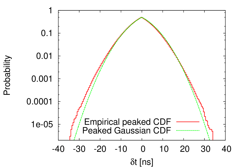
Figure 20: Empirical peaked CDF of $\delta t$ estimates from $10^{6}$ samples (red online) in comparison with the peaked Gaussian CDF of standard deviation 7.1 ns (green online).

As the distributions of the $\delta t_{k}$ are non-Gaussian, one may wonder whether Gaussian confidence limits provide a correct interpretation of the error bar (43). Indeed, the empirical peaked CDF [7] found for the $\delta t$ estimates via the direct method is broader than the Gaussian peaked CDF with standard deviation 7.1 ns. See Fig. 20, which relies for the empirical peaked CDF on $10^{6}$ random times samples. The largest fluctuation in the negative direction is at $-35.5\,$ns which has thus a probability of approximately $10^{-6}$. This is still safely away from $-57.8\,$ns.

Figure 21: Scatter plot of $(\delta\overline{t}^{i}_{1},\delta t^{i}_{1}-{\rm bias})$, $i=1,\dots,n$, $N=10\,000$ (model 1).

Finally in this section, we address correlations between the statistical fluctuations of $\delta\overline{t}_{k}$ and those of $\delta t_{k}$. Using $i=1,\dots,N=10\,000$ samples, for sample $i$ we denote $\delta\overline{t}_{k}$ by $\delta\overline{t}^{i}_{k}$ and $\delta t_{k}$ by $\delta t^{i}_{k}$. They have expectation values

$$\langle\delta\overline{t}_{k}^{i}\rangle_{7612}=\langle\delta t^{i}_{k}-{\rm bias}\rangle_{7612}=0\,.$$ (47)

The bias correction is so small that it can as well be ignored. Defining the correlation coefficients by

$$C(\delta\overline{t}_{k},\delta t_{k})\ =\ \frac{\sum_{i=1}^{n}\delta\overline{t}^{i}_{k}\,(\delta t^{i}_{k}-{\rm bias})}{\sum_{i=1}^{n}|\delta\overline{t}^{i}_{k}\,(\delta t^{i}_{k}-{\rm bias})|}$$ (48)

their calculation from our $10\,000$ samples gives

$$\langle C(\delta\overline{t}_{1},\delta t_{1})\rangle_{7612} = -0.47\,,$$ (49)

$$\langle C(\delta\overline{t}_{2},\delta t_{2})\rangle_{7612} = -0.43\,.$$ (50)

This, at the first glance, non-intuitive anti-correlation is for model 1 displayed in Fig. 21. It may be explained as follows. When $\delta\overline{t}$ fluctuates to negative values, there is an overpopulation of small $t$ values in the sample. Therefore a shift in the same direction has a higher probability to produce large negative contributions to the log-likelihood function (30) than a shift in the opposite direction.

7 Summary and Conclusions

We have investigated the problem of identifying a shift in a broad, non-Gaussian distribution of data. For two model probability densities (PD) shown in Fig. 1 methods are developed and illustrated to allow in samples of 7 612 MC generated departure times to identify a time shift with a precision of about $\pm 7.1\,$ns (even smaller than the error in our Eq.(1) from Ref. [1]). The noise of statistical fluctuations is with $\pm 23.8\,$ns much larger.

When the boundaries of the distribution are sufficiently sharp, uniform probabilities from binomials of the CDF provide excellent indicators. Subsequently it has been demonstrated that the maximum likelihood method gives a quantitative estimate of the shift $\delta t$ and its statistical error, while bootstrap simulations allow one to avoid Gaussian assumptions. Obviously, the analysis of this paper can be re-done for other desired sample sizes.

Acknowledgments: I would like to thank Peter Hoeflich for useful discussions and for extracting Fig. 1 from Fig. 11 of Ref. [1]. This work was in part supported by the DOE grant DE-FG02-13ER41942.

References

- [1] OPERA collaboration, arXiv:1109.4897v2.
- [2] OPERA collaboration, arXiv:1109.4897v4.
- [3] http://www.hep.fsu.edu/~berg/research/research.html
- [4] B. Efron, The Jackknife, the Bootstrap and other Resampling Plans, SIAM, Philadelphia 1982.
- [5] B.A. Berg and P. Hoeflich, arXiv:1110.2814.
- [6] G. Marsaglia, A. Zaman, and W.W. Tsang, Stat. Prob. 8 (1990) 35.
- [7] B.A. Berg, Markov Chain Monte Carlo Simulations and Their Statistical Analysis, World Scientific, 2004.
- [8] The sample used is just the first one encountered in our simulations.