Thermal constraints on the reionisation of hydrogen by population-II stellar sources

Abstract

Measurements of the intergalactic medium (IGM) temperature provide a potentially powerful constraint on the reionisation history due to the thermal imprint left by the photo-ionisation of neutral hydrogen. However, until recently IGM temperature measurements were limited to redshifts $2\leq z\leq 4.8$, restricting the ability of these data to probe the reionisation history at $z>6$. In this work, we use recent measurements of the IGM temperature in the near-zones of seven quasars at $z\sim 5.8-6.4$, combined with a semi-numerical model for inhomogeneous reionisation, to establish new constraints on the redshift at which hydrogen reionisation completed. We calibrate the model to reproduce observational constraints on the electron scattering optical depth and the H$\,\rm\scriptstyle I\$photo-ionisation rate, and compute the resulting spatially inhomogeneous temperature distribution at $z\sim 6$ for a variety of reionisation scenarios. Under standard assumptions for the ionising spectra of population-II sources, the near-zone temperature measurements constrain the redshift by which hydrogen reionisation was complete to be $z_{\rm r}>7.9$ $(6.5)$ at 68 (95) per cent confidence. We conclude that future temperature measurements around other high redshift quasars will significantly increase the power of this technique, enabling these results to be tightened and generalised.

1 Introduction

The reionisation of cosmic hydrogen represents a significant moment in the history of the Universe. The appearance of the first stars and quasars heated and ionised the IGM, catalysing the transition in which intergalactic hydrogen changed from being predominantly neutral to its present day, highly ionised state. Understanding exactly how and when this phase transition occurred will offer insight into the nature of the first sources of light (e.g. Barkana & Loeb 2001). However, existing constraints on the timescale and extent of reionisation are currently uncertain (Choudhury & Ferrara 2006; Pritchard et al. 2009; Mitra et al. 2011).

There are two primary observations which are used to constrain the epoch of hydrogen reionisation. The first of these are the absorption spectra of quasars at $z\simeq 6$ (White et al. 2003; Fan et al. 2006; Becker et al. 2007). These enable detailed study of the IGM ionisation state at high redshift, and indicate that the Universe was reionised at $z\geq 6$ (Gnedin & Fan 2006, but see also Mesinger 2010). The second observation is provided by measurements of the Thomson optical depth, ${\tau}_{\rm CMB}$, to the surface of last scattering, which indicate that hydrogen reionisation could not have ended any earlier than $z_{\rm r}=10.6\pm 1.2$ (Komatsu et al. 2011). In practice, this constraint is consistent with a wide variety of extended reionisation scenarios.

Analytical and semi-numerical models have been confronted with a combination of these and other observations to place more quantitative limits on the reionisation redshift. In particular, studies by Choudhury & Ferrara (2006), Pritchard et al. (2009) and Mitra et al. (2011) employ the above observables, alongside the observed distribution of Lyman limit systems and constraints on the star formation rate, to model reionisation. These models can be used to infer constraints on the extent and completion time of reionisation. However, the lack of direct observational evidence at $z>6$ means that parameters in these models, such as the ionising background intensity and the thermal state of the IGM, are relatively uncertain at high redshift. This implies that, from current observations alone, constraints on the redshift by which reionisation is complete remain loose, and cannot be improved beyond $6<z_{\rm r}<10.5$ (Mitra et al. 2011).

A promising additional approach comes from measurements of the IGM temperature (Zaldarriaga et al. 2001; Trac et al. 2008; Furlanetto & Oh 2009; Bolton et  al. 2010). The relatively long time scale of adiabatic cooling implies that the low redshift IGM still carries the thermal imprint of reionisation heating from much earlier times. Several authors have previously used this fact, combined with temperature measurements at $z<4$, to constrain the end of the hydrogen reionisation epoch to $z_{\rm r}<10$ (Theuns et al. 2002; Hui & Haiman 2003). Unfortunately, because the imprint of reionisation heating at $z_{\rm r}>10$ reaches a thermal asymptote by $z\approx 4$ these studies are limited by the relatively low redshift at which the temperature measurements were made.

Measurements of IGM temperature at higher redshift therefore offer a new opportunity to tighten these constraints. A first step towards this was made by Bolton et  al. (2010), who obtained a measurement of the IGM temperature at mean density from Ly$\alpha$ absorption lines in the near-zone of the $z=6.02$ quasar SDSS J0818$+$1722. Although the statistical uncertainty on their single line-of-sight measurement was large, Bolton et  al. (2010) were nevertheless able to use a simple cooling argument to infer a reionisation redshift of $z_{\rm r}<9$ (to 68 percent confidence) within the quasar near-zone, assuming hydrogen was reionised by population-II stars. Recently, Bolton et  al. (2011) have significantly extended these observational constraints by measuring the IGM temperature in the near-zones of six further quasars at $5.8\leq z\leq 6.4$. In this work, we therefore seek to extend the modelling of Bolton et  al. (2010) and include all seven near-zone temperature measurements to obtain a limit on the reionisation redshift for the general IGM. Specifically, by using a semi-numerical model to follow inhomogeneous reionisation and photo-heating of intergalactic hydrogen by stellar sources, as well any subsequent photo-heating by the quasar itself, we may calculate near-zone temperatures as a function of spatial position and reionisation redshift. A comparison of our model with the observational data then allows us to constrain the redshift at which reionisation completed.

The paper is organised as follows. We begin in Section 2 by introducing our semi-numerical model of reionisation, and proceed in Section 3 to give a more detailed description of the modelling of ionising sources. Predicted temperatures from the model for different reionisation scenarios are then described in Section 4, and we compare these to the Bolton et  al. (2011) quasar temperature measurements. Our constraints on reionisation history are then discussed in Section 5, where we also assess the prospects for improving on these constraints in the future using additional quasar sight-lines. Conclusions and further directions are then presented in Section 6. Throughout the paper we use $\Lambda$CDM cosmological parameters $\Omega_{\rm m}=0.27$, $\Omega_{\Lambda}=0.73$, $\Omega_{\rm b}h^{2}=0.0225$, $h=0.704$, $\sigma_{8}=0.81$, $n_{\rm s}=0.96$, consistent with recent studies of the cosmic microwave background (Komatsu et al. 2011).

2 Semi-Numerical Reionisation Model

Our model of inhomogeneous hydrogen reionisation simulates both the evolving ionisation state of the IGM and its thermal history. The former is calculated using the semi-numerical model developed by Wyithe & Loeb (2007) and Geil & Wyithe (2008) (see also Zahn et al. 2007; Mesinger & Furlanetto 2007; Choudhury et al. 2009; Thomas et al. 2009 for similar approaches). The ionisation state derived from this model is then used to evaluate both the ionising flux and the mean free path at the Lyman Limit, and to infer a temperature distribution for the IGM.

2.1 Ionisation model

We simulate the IGM inside a periodic, cubic grid of side-length $L=100\,{h^{-1}\,\rm Mpc}$, containing $N=256$ voxels per side-length, with an over-density field ${\delta}(x)$ generated using the transfer function of Eisenstein & Hu (1999). The calculations detailing the evolution of ionisation structure in this density field (which is initialised to a neutral state at $z=99$) are described in Geil & Wyithe (2008). Briefly, the model evaluates the ionisation fraction $Q_{\delta_{R},R}$ of a spherical region of scale $R$ around a given voxel at redshift $z$ as

$$\frac{dQ_{\delta_{R},R}}{dt} = \frac{N_{\rm ion}}{0.76}\left[Q_{\delta_{R},R}\frac{dF_{\rm col}(\delta_{R},R,z,M_{\rm ion})}{dt}\right.$$ (1)

$$+ \left.\left(1-Q_{\delta_{R},R}\right)\frac{dF_{\rm col}(\delta_{R},R,z,M_{\rm min})}{dt}\right]$$

$$- \alpha_{\rm B}Cn_{\rm H}^{0}\left[1+\delta_{R}\frac{D_{1}(z)}{D_{1}(z_{\rm obs})}\right]\left(1+z\right)^{3}Q_{\delta_{R},R},$$

where ${\delta_{R}}$ is the region’s over-density, $\alpha_{\rm B}$ is the case-B recombination coefficient and $C$ is the clumping factor. In this work we shall assume $C=3$, broadly consistent with recent results from hydrodynamical simulations (Pawlik et al. 2009; Raicević & Theuns 2011). The justification for this choice, as will be discussed in more detail in Section 5.1, is that it tends to provide the weakest overall constraints on reionisation redshift. Meanwhile, $N_{\rm ion}$, the number of ionising photons entering the IGM per baryon in galaxies, is left as a free parameter, the modelling of which will be described in more detail in Section 3.

The production rate of ionising photons is then assumed to be proportional to $N_{\rm ion}$ and the rate of change of the collapsed fraction, $F_{\rm col}$, in haloes above some minimum threshold mass for star formation ($M_{\rm min}$ in neutral and $M_{\rm ion}$ in ionised regions, corresponding to virial temperatures of $10^{4}$ K and $10^{5}$ K respectively, e.g. Dijkstra et al. 2004). The collapsed fraction in a region of comoving radius $R$ and mean overdensity $\delta(z)=\delta(z_{\rm obs})D_{1}(z)/D_{1}(z_{\rm obs})$ is found using the extended Press-Schechter model (Bond et al., 1991), which gives

$$F_{\rm col}(\delta_{R},R,z)=\mbox{erfc}{\left[\frac{\delta_{c}-\delta_{R}(z)}{\sqrt{2(\sigma^{2}_{\rm gal}-\sigma_{R}^{2})}}\right]},$$ (2)

where $\mbox{erfc}(x)$ is the complimentary error function, $\sigma_{R}^{2}$ is the variance of the overdensity field smoothed on a scale $R$ and $\sigma^{2}_{\rm gal}$ is the variance of the overdensity field smoothed on a scale $R_{\rm gal}$, corresponding to a mass scale of $M_{\rm min}$ or $M_{\rm ion}$ (both evaluated at redshift $z$).

Equation (1) is solved at every voxel on a range of scales from $L$ to $L/N$ at logarithmic intervals of width $\Delta R/R=0.1$. A voxel is then deemed to be ionised if it lies inside a region for which $Q_{\delta_{R},R}>1$ on any scale $R$. By repeating this procedure at successive redshifts, we obtain our ionisation field as a function of $z$.

2.2 The ionising emissivity

In order to compute the heating of the IGM, we must next obtain the ionising emissivity in each voxel of our simulation. We simulate the ionisation field at 30 regular redshift intervals between an initial redshift, $z_{\rm 0}$, and the reionisation redshift, $z_{\rm r}$. These are, respectively, the redshifts corresponding to $Q=0.01$ and $Q=1.0$, where $Q=Q_{\delta_{R},R}$ for the case where equation (1) is solved at mean density and $R\rightarrow\infty$. At each interval, if a voxel is flagged as ionised, we compute the intrinsic emissivity as the product of $N_{\rm ion}$ and the collapsed fraction above a minimum halo mass, $M_{\rm ion}$. Using this, the proper ionising photon production rate ($\dot{N_{\rm{\gamma}}}$) in units of photons ${\rm cm^{-3}}{\,\rm s^{-1}}$, at each voxel, is

$$\dot{N_{\rm{\gamma}}}=\frac{{\rho}_{\rm c}{\Omega}_{\rm b}(1+z)^{3}(1+\delta_{\lambda})N_{\rm ion}}{{\mu}m_{\rm p}}\frac{dF_{\rm col}(\delta_{\lambda},{\lambda_{\rm HI}},z,M_{\rm ion})}{dt},$$ (3)

where ${\rho}_{\rm c}$ is the present day critical density, $m_{\rm p}$ is a proton mass and ${\mu}$ is the mean molecular weight. In this instance, the smoothing scale $\lambda$ used to calculate the collapsed fraction is given by the minimum of the ionised bubble radius and the mean free path at the Lyman limit, ${\lambda_{\rm HI}}$. This is related to the ionising emissivity $\epsilon_{\nu}$, (in units of $\rm erg\,s^{-1}\,cm^{-3}\,Hz^{-1}$) above the Lyman Limit frequency, ${\nu_{\rm HI}}$, by

$$\dot{N_{\rm{\gamma}}}=\int_{\nu_{\rm HI}}^{\infty}\frac{\epsilon_{\nu}}{h_{\rm p}\nu}\,d\nu,$$ (4)

where we adopt a simple power law spectrum

$$\epsilon_{\nu}=\left(\frac{\nu}{\nu_{\rm HI}}\right)^{-\alpha}\times\cases{\epsilon_{\rm HI}&($\nu_{\rm HI}\leq\nu<\nu_{\rm HeII}$),\cr\vskip 3.0pt\cr 0&($\nu_{\rm HeII}\leq\nu$).\cr}$$ (5)

Here $\epsilon_{\rm HI}$ is the emissivity at the hydrogen Lyman limit. Below the He$\,\rm\scriptstyle II\$ionisation edge, we take a spectral index of ${\alpha}=3$ characteristic of soft, population-II stellar sources (e.g. Hui & Haiman 2003; Furlanetto & Oh 2009). Above ${\nu}_{\rm HeII}$, the spectrum is zero in order to enforce the requirement that there be no significant stellar ionisation of He $\rm\scriptstyle II$. This is necessary for consistency with our semi-numerical reionisation model which only traces the propagation of hydrogen ionisation fronts, and so cannot predict the larger, extended He$\,\rm\scriptstyle III\$fronts resulting from harder He$\,\rm\scriptstyle II\$ionising photons. On the other hand this is not an unrealistic requirement, since the double reionisation of helium is thought to not complete until $z\sim 3$ when the number density of quasars is at its peak (Madau & Meiksin 1994; Wyithe & Loeb 2003; Furlanetto & Oh 2008). Nevertheless, this assumption rules out the consideration of more exotic ionisation models involving early populations of quasars or population-III sources, which could produce different thermal histories. More detailed modelling, which accounts for doubly ionised helium may therefore be performed in the future. In this work, however, we consider hydrogen reionisation by population-II stellar sources only.

2.3 The ionising background specific intensity

Having computed the intrinsic emissivity, the specific intensity, $J_{\rm{\nu}}$, at each voxel may then be calculated by accounting for the propagation and attenuation of radiation. This is a complicated calculation since, in general, it depends on the topology of H$\,\rm\scriptstyle II\$regions around each point in the simulation and the distribution of Lyman limit systems. A full numerical evaluation therefore requires radiative transfer, which is not included in our model. Fortunately, the long-term thermal evolution (for timescales longer than the local photo-ionisation timescale) is relatively insensitive to the exact amplitude of $J_{\rm{\nu}}$, and instead depends primarily on the spectral shape of the ionising radiation (Hui & Haiman 2003; Bolton et al. 2009). Therefore, to estimate the specific intensity we make the simplifying assumption that the mean free path is much smaller than the horizon scale, and use the local source approximation (e.g. Faucher-Giguère et al. 2009). We compute the mean free path in two regimes, prior to and following the overlap of H$\,\rm\scriptstyle II\$regions.

Prior to overlap, the mean free path is set by the size of H$\,\rm\scriptstyle II\$bubbles (Gnedin & Fan 2006), and may therefore be found by partitioning the ionisation field into approximately spherical H$\,\rm\scriptstyle II\$regions. To do this, we smooth over the ionisation field at successive scales, employing the same logarithmic descent as for our density field. At each scale we calculate the size of discontiguous regions with a standard friend-of-friends (FoF) algorithm. The bubble size for each voxel is then the scale of the smallest FoF region of which it is part, augmented by the smoothing scale. This has the effect of dividing bubbles that only barely overlap into separate spheres so that the spherical approximation remains valid to a filling factor of around $Q\approx 0.5$. We then assume that the optical depth to ionising photons is infinite beyond the H$\,\rm\scriptstyle II\$region radius. Lyman Limit photons therefore travel one mean free path, corresponding to the H$\,\rm\scriptstyle II\$region size, before being absorbed.

In the post-overlap case, the IGM is fully ionised and the mean free path of H$\,\rm\scriptstyle I\$ionising photons is constrained by the abundance of Lyman limit systems rather than the sizes of H$\,\rm\scriptstyle II\$regions. In this instance, we employ a fit to the mean-free-path at the Lyman limit in proper Mpc, taken from Songaila & Cowie (2010):

$${\lambda_{\rm HI}}=\frac{88.6}{\Gamma(2-\beta)}{\left(\frac{1+z}{4.5}\right)}^{-4.44}{\rm Mpc},$$ (6)

where $\Gamma$ denotes the gamma function, and ${\beta}$ is the power law exponent of the H$\,\rm\scriptstyle I\$column density distribution. Observationally, the value of this exponent is unconstrained at $z>6$, however at lower redshift measurements indicate $\beta\approx 1.5$ (Petitjean et al., 1993; Hu et al., 1995). Since this is roughly constant over the range $2<z<4$ (Misawa et al., 2007), we simply extrapolate to high redshift and adopt $\beta=1.5$ throughout. We note that the column density distribution will change significantly as we enter the reionisation epoch, however as we are primarily interested in the value of $\beta$ in the post-overlap regime, this does not affect our results. Finally, we assume that a given H$\,\rm\scriptstyle II\$region is in the pre-overlap regime if its radius is less than ${\lambda_{\rm HI}}$ (i.e. the mean free path is not set by Lyman limit systems) and is in the post-overlap regime otherwise.

Adopting the local source approximation, the ionising background specific intensity in each voxel may then be approximated by

$$J_{\nu}\simeq\frac{1}{4\pi}\epsilon_{\nu}\lambda_{\nu},$$ (7)

where $\lambda_{\nu}=\lambda_{\rm HI}(\nu/\nu_{\rm HI})^{3(\beta-1)}$. Prior to overlap $\lambda_{\rm HI}$ is fixed to the H$\,\rm\scriptstyle II\$region size, while post overlap it is given by equation (6). Lastly, note that in both regimes at frequencies above the Lyman Limit, we have $J_{\nu}\propto\nu^{-\alpha+3(\beta-1)}$. This effectively hardens the intrinsic stellar spectrum by $\alpha\rightarrow\alpha-1.5$ , accounting for the additional heating due to filtering of the ionising radiation by discrete, Poisson distributed absorbers in the intervening IGM (e.g. Miralda-Escudé 2003; Faucher-Giguère et al. 2009).

2.4 The thermal evolution

Once the specific intensity at a given voxel is known, the photo-ionisation rates, $\Gamma_{\rm i}\rm\,[s^{-1}]$, and photo-heating rates, $g_{\rm i}\rm\,[erg\,s^{-1}]$, for $i$=H $\rm\scriptstyle I$, He $\rm\scriptstyle I$ and He $\rm\scriptstyle II$, may be calculated via:

$${\Gamma_{\rm i}}=\int_{\nu_{\rm i}}^{\infty}\frac{4{\pi}J_{\rm\nu}}{h_{\rm p}\nu}{\sigma_{\rm i}}({\nu})d\nu,$$ (8)

$${g_{\rm i}}=\int_{\nu_{\rm i}}^{\infty}\frac{4{\pi}J_{\rm\nu}}{h_{\rm p}\nu}h_{\rm p}(\nu-\nu_{\rm i}){\sigma_{\rm i}}({\nu})d\nu,$$ (9)

where ${\sigma_{\rm i}}({\nu})$ and $\nu_{\rm i}$ are the photoionisation cross-section and frequency at the ionisation edge for species $i$, respectively. The temperature evolution is then computed by solving:

$$\frac{dT}{dt}=\frac{(\gamma-1){\mu}m_{\rm p}}{k_{\rm B}{\rho}}\left[G(t)-\Lambda(t,n_{\rm i})\right]-2H(t)T+\frac{T}{\mu}\frac{d{\mu}}{dt},$$ (10)

where $\gamma=\frac{5}{3}$, and $G=\sum_{\rm i}n_{\rm i}g_{\rm i}$ and $\Lambda$ are the total photo-heating and cooling rates per unit volume, respectively. We ignore any heating resulting from the growth of density fluctuations as this is a minimal effect throughout the short timescale of reionisation. Our code for solving equation (10) follows photo-ionisation and heating, collisional ionisation, radiative cooling, Compton cooling and adiabatic cooling for six species (H $\rm\scriptstyle I$, H $\rm\scriptstyle II$, He $\rm\scriptstyle I$, He $\rm\scriptstyle II$, He $\rm\scriptstyle III$, $\rm e^{-}$). The non-equilibrium abundances of these species are found by additionally solving three further differential equations coupled to equation (10) (e.g. Anninos et al. 1997; Bolton & Haehnelt 2007), and taking a uniform clumping factor of $C=3$ for all species. We use the rates compiled in Bolton & Haehnelt (2007) with the exception of the case-B recombination and cooling rates of Hui & Gnedin (1997) and the photo-ionisation cross-sections of Verner et al. (1996). The gas density, $\rho$, is evaluated from our linear over-density field using a standard log-normal fit (Coles & Jones 1991), which approximates the real non-linear density for the majority of voxels. Whilst this does not adequately reproduce the extreme over-dense and underdense tails of the density distribution (Becker et al. 2007), its use does not represent a significant source of error since the temperature measurements we compare to are smoothed over the measured quasar near-zones ($\sim 5$ proper Mpc). Inaccuracies in evaluating the thermal history of the small number of regions that fall within these tails are therefore unimportant.

Using this prescription, we evolve the temperature of each voxel, independent of all others from an initial temperature $T_{\rm 0}=2.27(1+z){\rm K}$ and an initially neutral state. This procedure yields a final temperature distribution over our simulation volume as a function of redshift.

2.5 Inclusion of quasar He$\,\rm\scriptstyle II\$photo-heating

The final part of our model is including the effect of the quasars themselves on the thermal state of the IGM in their vicinity. The ionising flux from a quasar will significantly alter the thermal state of the surrounding IGM, as its harder, non-thermal spectrum will also reionise He $\rm\scriptstyle II$ (Bolton et  al. 2010). For any given quasar from Bolton et  al. (2011), placed in the simulation volume at a random position, we account for this heating by augmenting the specific intensity in each voxel within the quasar proximity zone by an additional term

$$J_{{\nu},\rm q}\simeq\frac{L_{\nu}}{(4\pi R)^{2}}\exp\left[-\frac{R}{\lambda_{\rm HI}}\left(\frac{\nu}{\nu_{\rm HI}}\right)^{-3(\beta-1)}\right],$$ (11)

where $R$ is the proper distance from the quasar and $L_{\nu,\rm q}=L_{\rm HI,q}(\nu/\nu_{\rm HI})^{-\alpha_{\rm q}}$ is the quasar ionising luminosity, again taken to be a power law spectrum with index ${\alpha_{\rm q}}$. There is considerable uncertainty concerning the exact value of this exponent towards high redshift. We therefore allow it to vary over the range $1.0\leq\alpha_{\rm q}\leq 2.0$, which is consistent with recent indirect estimates from observations of quasar near-zone sizes at $z>6$ (Wyithe & Bolton 2011). To compute the quasar luminosities at the Lyman limit, we take the absolute AB magnitudes from Carilli et al. (2010). Finally, we fix the extent of the region which experiences additional ionisation and heating by each quasar to 5 proper Mpc, matching the radius within which the near-zones were analysed in Bolton et  al. (2011).

3 Modelling of ionising sources

We next discuss the parametrisation of ionising sources in our model, encapsulated by the redshift-dependent parameter $N_{\rm ion}$, the number of ionising photons entering the IGM per baryon in galaxies. We begin by describing existing observational constraints on the IGM ionisation state and then proceed to discuss how these are used to calibrate $N_{\rm ion}$ and its evolution with redshift.

3.1 Observational constraints on $N_{\rm ion}$

3.1.1 The ionisation rate from the Ly$\alpha$ forest opacity

Table 1: Photo-ionisation rate constraints from the Ly$\alpha$ forest opacity obtained by Bolton et  al. (2005) and Wyithe & Bolton (2011). The most likely derived value and errors at 68 per cent confidence intervals for the corresponding number of ionising photons entering the IGM per baryon in galaxies, $N_{\rm ion}$, are also given.

Redshift	$\Gamma_{\rm-12}$	$N_{\rm ion}$
4	$0.97\pm^{0.48}_{0.33}$	$35.3\pm^{17.5}_{12.1}$
5	$0.47\pm^{0.3}_{0.2}$	$22.7\pm^{14.3}_{9.7}$
6	$0.18\pm^{0.18}_{0.09}$	$13.0\pm^{13.0}_{6.5}$

Observations of the Ly${\alpha}$ forest in quasar absorption spectra can be used to infer the ionising background due to luminous sources. The measured quantity is the mean transmission of Ly${\alpha}$ flux, $\left<F\right>$, along the line of sight, or equivalently the effective optical depth ${\tau}_{\rm eff}=-{\rm log}\left<F\right>$. With knowledge of the physical properties of the IGM, these can be converted into the background photoionisation rate per hydrogen atom (${\Gamma}_{\rm HI}={\Gamma}_{\rm-12}\times 10^{-12}{\rm\,s^{-1}}$). Using full hydrodynamical simulations of the IGM, Bolton et  al. (2005) and Wyithe & Bolton (2011) have measured $\Gamma_{\rm-12}$ from the Ly$\alpha$ forest opacity at $z=4-6$. Their derived values are shown in Table 1. These measurements may then be compared to our own simulated ionisation rate, which is calculated using equation (8). When combined with equations  (3)–(7), and evaluated for the case of a uniformly ionised IGM at $z<6$ this yields constraints on $N_{\rm ion}$, which are also shown in Table 1.

3.1.2 Thomson optical depth to CMB photons

The electron scattering optical depth provides an integrated constraint on the IGM ionisation state throughout the epoch of reionisation. We use results from the latest WMAP observations, ${\tau}_{\rm CMB}=0.088\pm 0.015$ (Komatsu et al. 2011). This is related to the ionisation history by

$${\tau}_{\rm CMB}=\int_{0}^{z_{\rm CMB}}c\frac{dt}{dz}Q(z)\left(1+f_{\rm He}(z)\right)n_{\rm H}(z){\sigma_{\rm T}}dz,$$ (12)

where ${\sigma_{\rm T}}$ is the Thomson scattering cross-section, $n_{\rm H}$ is the hydrogen number density and $f_{\rm He}$ is a correction factor due to the presence of ionised helium. In our model, we assume that the ionisation of He$\,\rm\scriptstyle I\$traces that of H$\,\rm\scriptstyle I$, whilst He$\,\rm\scriptstyle II\$is instantaneously ionised at $z=3$.

3.2 Parametrisation of $N_{\rm ion}$

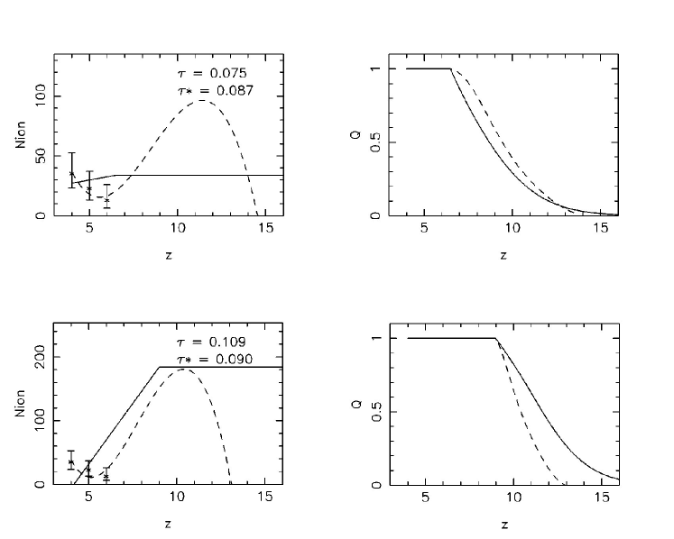
Figure 1: Evolution of the number of ionising photons per baryon in galaxies which escape into the IGM, $N_{\rm ion}$ (left hand columns), and the H$\,\rm\scriptstyle II\$filling factor, $Q$ (right hand columns) for reionisation histories with $z_{\rm r}=6.5$ (top) and $z_{\rm r}=9.0$ (bottom). Solid curves show the evolution for the linear $N_{\rm ion}$ model, whilst the case of the cubic $N_{\rm ion}$ is shown by the dashed lines. The plotted points represent constraints imposed by values of ${\Gamma_{\rm-12}}$ obtained from the Ly$\alpha$ forest opacity by Bolton et  al. (2005) and Wyithe & Bolton (2011). The inset in the left hand panels gives the electron scattering optical depth for the linear and cubic $N_{\rm ion}$ models ($\tau$ and $\tau*$, respectively).

Using these observations, we may now constrain possible parametrisations of $N_{\rm ion}$ in our model. There is considerable uncertainty concerning the exact shape of $N_{\rm ion}$, particularly for $z>6$, where there are no direct observations. Indeed, several studies (Pritchard et al. 2009; Mitra et al. 2011) have found that $N_{\rm ion}$ is effectively unconstrained in the range $6<z<11$. To explore the sensitivity of our simulated temperatures to changes in the ionising sources, we therefore choose to employ two different models for the redshift evolution of $N_{\rm ion}$.

3.2.1 Linear model

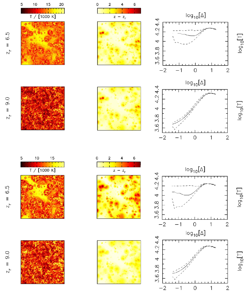
Figure 2: Maps of a two-dimensional slice through the centre of our $100h^{-1}$ comoving Mpc simulation box at $z=6.0$ prior to the inclusion of any quasar heating. The upper six panels show results for the linear $N_{\rm ion}$ model while the lower set show the same results allowing for a cubic $N_{\rm ion}$. In each set, the upper row indicates maps for reionisation occurring at $z_{\rm r}=6.5$ and the lower row for $z_{\rm r}=9.0$. Left panels: The IGM temperature at the measurement redshift ($z=6.0$). Central Panels: Maps of the ionisation redshift for each voxel relative to the redshift at which reionisation completes, $\Delta z=z-z_{\rm r}$. Right panels: The IGM temperature, T, against overdensity, $\Delta$, at $z=6.0$, displaying both the median (solid) and 68 per cent intervals around the median (dashed).

The simplest model, and one often used in previous simulations of reionisation (e.g. Haiman & Loeb 1997; Geil & Wyithe 2008), assumes a single, redshift independent parametrisation of $N_{\rm ion}$. However, this cannot be reconciled with measurements of the photo-ionisation rate from the Ly$\alpha$ forest at $z\leq 6$, so we employ a slight variant on the model. We take $N_{\rm ion}$ to be a constant up to the reionisation redshift, which is found by solving equation (1) for a universe that is fully ionised by the desired redshift. This effectively fixes the reionisation history for any given $z_{\rm r}$. Then, to ensure consistency with observations of $\Gamma_{\rm-12}$, we allow $N_{\rm ion}(z)$ to evolve linearly once reionisation is complete in order to best fit the data points at $z<6$. This is broadly consistent with predicted increases in the escape fraction towards high redshift (Wyithe et al. 2010). As part of our constraint on $z_{\rm r}$ we impose the resulting electron scattering optical depth as an a posteriori constraint on $z_{\rm r}$ alongside the predicted temperatures in Section 5.

3.2.2 Cubic Model

We also explore arbitrary ionisation histories that best match the ${\tau}_{\rm CMB}$ constraint, by employing a model that is redshift-dependent prior to $z_{\rm r}$. To ensure enough freedom to match all constraints, we choose to follow the approach of Pritchard et al. (2009) and model $N_{\rm ion}$ as a cubic function, allowing for a large variety of different evolutions:

$$N_{\rm ion}(z)=\left(N_{\rm p}-N_{\rm 0}\right)\left[4\left(\frac{z-z_{\rm 0}}{\Delta z}\right)^{3}-3\left(\frac{z-z_{\rm 0}}{\Delta z}\right)\right]+N_{\rm 0},$$ (13)

where we have parametrised by the midpoint $\left(z_{\rm 0},N_{\rm 0}\right)$, and the peak $\left(z_{\rm 0}+\frac{\Delta z}{2},N_{\rm p}\right)$. For each reionisation redshift, we fit this curve to the measured electron scattering optical depth and the ionisation rate at $z=4-6$. As in Pritchard et al. (2009), we impose a prior on the comoving emissivity of $\dot{N_{\rm\gamma}}<10^{51}{\rm\,s^{-1}}{\rm Mpc^{-3}}$ to disallow unphysically large ionising backgrounds. We stress that this model is not physically motivated and clearly overfits the limited data we use. However, as we do not seek to exactly find $N_{\rm ion}$ but only to view the effect of different ionisation histories on simulated IGM temperatures, this does not significantly impact upon our results.

3.2.3 Optimal $N_{\rm ion}$ models

Finally, the best fit evolution of $N_{\rm ion}$ and the filling factor $Q$ for the cubic and linear models are shown in Figure 1 for $z_{\rm r}=6.5$ and $z_{\rm r}=9.0$. For both cases, the behaviour of the emissivity matches quite well to results derived elsewhere (Choudhury & Ferrara 2006; Pritchard et al. 2009; Mitra et al. 2011), although note that for early reionisation in the cubic model, star formation switches on later and the filling factor develops more quickly in order to match the electron scattering constraint. Importantly, the two models do provide very different ionisation histories at each $z_{\rm r}$ and therefore should allow us to probe the sensitivity of our temperature predictions to realistic variations in the ionising background.

4 Results of the semi-numerical model

4.1 The IGM thermal state following hydrogen reionisation

We now examine the variation of IGM temperature with reionisation redshift using the semi-numerical model described in the previous two sections. For any given $z_{\rm r}$, and for each of the two different parametrisations of $N_{\rm ion}$, we compute an optimal $N_{\rm ion}$ evolution that ensures $Q=1.0$ by $z_{\rm r}$. The resulting ionising background then allows us to calculate the temperature field over the redshift range $5.5<z<6.5$, when the quasars analysed in Bolton et  al. (2011) are expected to have had their most recent optically bright phase.

The IGM temperatures predicted by our semi-numerical model at $z=6.0$ are summarised in Figure 2. The top two rows display the results using our linear $N_{\rm ion}$ model, for reionisation completing by $z_{\rm r}=6.5$ (first row) and $z_{\rm r}=9.0$ (second row). The left hand panels display temperature maps through the centre of the $100h^{-1}$ Mpc simulation volume. The corresponding central panels show maps of the voxel ionisation redshifts relative to the redshift at which reionisation completes (i.e. $\Delta z=z-z_{\rm r}$). We note that the structure of ionised bubbles at fixed $\Delta z$ is very similar for the early and late models. In the case of late reionisation, the temperature mimics this ionisation structure, with cooler regions centred on the small H$\,\rm\scriptstyle II\$bubbles that were ionised first, and have thus had more time to cool. However, regions of the IGM ionised during the overlap phase retain a clear imprint of heating. The situation is very different for early reionisation, where the temperature field shows little correlation with the reionisation topology. Instead, the temperature largely reflects the random Gaussian structure of the density field, indicating that even with reionisation occurring at $z_{\rm r}=9.0$, the temperature has already settled to an almost asymptotic state by $z=6.0$.

This asymptotic limit is also clear from the temperature-density relation (right hand panels of Figure 2). For $z_{\rm r}=9.0$, the relation shows an almost power law dependence with $\gamma-1\approx 0.5$ for $T=T_{\rm 0}\Delta^{\gamma-1}$, characteristic of an asymptotic IGM thermal state which is set by the competition between photo-heating and adiabatic cooling (Hui & Gnedin, 1997). However, in the case of late reionisation, the figure shows much wider 68 per cent confidence limits (dashed lines) below the highest densities, with an inverted power-law slope of $\gamma-1\approx-0.2$ for low densities ($\Delta<1.0$). The scatter and anti-correlation between temperature and density, which arises due to the fact that lower density regions tend to be ionised last allowing them less time to cool, is in qualitative agreement with results from previous numerical and analytical studies (Bolton et al. 2004; Trac et al. 2008; Furlanetto & Oh 2009).

The same set of results can also be seen for the cubic model of $N_{\rm ion}$ in the two lower rows in Figure 2. In this case, the growth of ionised bubbles is significantly different at constant $\Delta z=z-z_{\rm r}$ for the two reionisation redshifts. As described in Section 3.2, late reionisation ($z_{\rm r}=6.5$) is a more gradual process in this model, with ionisation times spread more evenly around the H$\,\rm\scriptstyle II\$bubbles. This has the effect of spreading out the IGM temperatures, so that regions ionised early tend to be cooler. Similarly, the scatter in the temperature-density relation is increased. On the other hand, for $z_{\rm r}=9.0$, reionisation is far more rapid, effectively occurring over a redshift interval of ${\Delta}z=3.0$. Despite this difference, the temperature field evolves, by $z=6.0$, to the same asymptotic state as for the linear $N_{\rm ion}$ model (with a slightly reduced scatter in the temperature-density relation due to the more abbreviated differences in ionisation time). This reaffirms the conclusion that the thermal memory of hydrogen reionisation for $z_{\rm r}=9.0$ is largely erased by $z=6.0$.

To see this more clearly, in Figure 3 we consider how the mean and standard deviation of the temperature distribution at $z=6.0$ evolve as a function of reionisation redshift. We note that the mean referred to here is not directly comparable to the measurements of Bolton et  al. (2011) as it is averaged over the entire density field in the simulation volume and is not simply the temperature at mean density. The results are shown for both the linear (solid red) and cubic (dashed blue) $N_{\rm ion}$ models. The mean temperature predicted by the two models only varies by several hundred degrees Kelvin above $z_{\rm r}\approx 9.0$, and an asymptotic state is fully reached for $z_{\rm r}\approx 10.5-11.0$. However, for later reionisation redshifts the temperature distributions vary quite rapidly, and for the linear $N_{\rm ion}$ model at $z_{\rm r}=6.0$ the IGM is $\sim 5000\rm\,K$ hotter than the asymptotic value. This result is slightly more muted for the cubic model, as the elongated reionisation history means that large regions of the IGM have longer to cool, thereby reducing the impact of heating on the mean temperature. However, even allowing for this, unit changes in the reionisation redshift correspond to temperature variations of up to $1500\rm\,K$ by $z=6.0$. As this is comparable to the standard deviation of the distributions, changes of ${\Delta}{z_{\rm r}}\approx 1.0$ should be distinguishable on the basis of volume averaged temperature measurements for $z_{\rm r}<9.0$, but will require very precise data.

Finally, note that the standard deviation exhibits a minimum at $z_{\rm r}\sim 7$ for both models, but increases to both lower and higher redshift. At $z_{\rm r}<7$, this scatter is driven by the large variation in temperatures resulting from recent, inhomogeneous reionisation. In contrast, the scatter at $z_{\rm r}>7$ is instead due to the steepening correlation between temperature and density which establishes itself following reionisation. Both models asymptotically approach a value of $\sigma(T)\sim 3000\rm\,K$ for $z_{\rm r}\ga 10$.

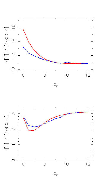
Figure 3: Mean (top panel) and standard deviation (bottom panel) of the simulated temperature distributions at $z=6.0$ prior to the inclusion of quasar heating. Note the results are obtained from the entire $100h^{-1}$ comoving Mpc simulation box, and the mean is therefore volume averaged over all densities. We show results for two different cases; the linear $N_{\rm ion}$ model (solid red curves) and the cubic model allowing for an evolving $N_{\rm ion}$ (dashed blue curves).

4.2 The temperature in quasar near-zones

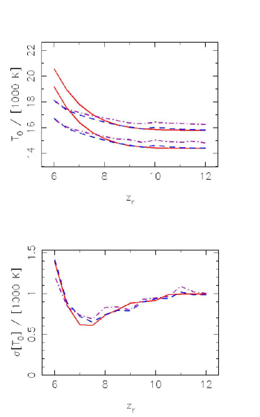
Figure 4: Mean and standard deviation of the simulated distributions over temperature at mean density, $p(T_{\rm 0}|z_{\rm r})$, in a quasar proximity zone at $z=6.02$. Top: Simulated mean for three different cases, the linear $N_{\rm ion}$ model (solid lines), the cubic model (dashed lines), and the cubic model accounting for the density bias of quasars (dot-dashed lines). We show simulated temperatures for $\alpha_{\rm q}=2.0$, which yield the lower curves and $\alpha_{\rm q}=1.0$ giving the higher set of curves. Bottom: Standard deviations for the aforementioned models. In this case we only show results for $\alpha_{\rm q}=1.0$, however standard deviations are similar regardless of quasar spectral index.

Bolton et  al. (2011) used the Doppler parameters of H$\,\rm\scriptstyle I\$Ly$\alpha$ absorption lines in the near-zones of 7 quasars at $5.8<z<6.4$ to measure the IGM temperature at mean density, $T_{0}$, within $\sim 5$ proper Mpc of these sources. In order to compare these observations to our model, we must therefore also include the effect of He$\,\rm\scriptstyle II\$photo-heating by the quasars themselves on the IGM temperature.

We calculate this heating as follows. At any given voxel in our simulation volume, we switch on a quasar $t_{\rm q}=1.5\times 10^{7}$ yrs prior to the redshift at which the quasar is observed, and use the procedure outlined in Section 2.5 to calculate the surrounding IGM temperature. We then draw 200 random lines-of-sight within a $\sim 5$ proper Mpc region around the quasar, and for each one we measure the temperature-density relation for all voxels. This relation may then be used to infer a temperature at mean density averaged over all 200 lines-of-sight. Repeating this procedure for “quasars” centred on all voxels in the simulation box then gives a distribution for the temperatures around a single observed quasar.

In Figure 4 we show the mean and standard deviation of the simulated temperature distributions at mean density for a quasar observed at $z=6.02$. The results for the mean temperature are displayed for both hard ($\alpha_{\rm q}=1.0$, upper curves) and soft ($\alpha_{\rm q}=2.0$, lower curves) quasar spectral indices. The red solid and blue dashed curves again correspond to the linear and cubic $N_{\rm ion}$ models. These retain all the features of the temperature distributions prior to quasar heating, including the asymptotic behaviour of the mean at $z_{\rm r}\ga 9.0$, and the minimum in the scatter at $z_{\rm r}\simeq 7.0$. Note, however, the standard deviation tends to be slightly smaller, particularly at large $z_{\rm r}$. This is due to the fact that we are now only considering the average temperature at a single (mean) density.

We find that the maximum difference in the average temperature at mean density for the cubic $N_{\rm ion}$ model is only $\sim 2\,500{\rm K}$ for early and late reionisation. Given that the 68 per cent measurement uncertainties on the temperature around individual quasars obtained by Bolton et  al. (2011) are $\sim 3\,000$–$5\,000{\rm K}$, it is unlikely that a strong constraint can be obtained from any single line-of-sight observation. However, the combination of all 7 quasars analysed by Bolton et  al. (2011) reduces the 68 per cent confidence interval on the mean temperature of the quasar near-zones to $\sim 1\,500{\rm K}$. Therefore, all seven lines-of-sight will be able, in principle, to distinguish between early and late reionisation scenarios.

It is important to note that the rather uncertain quasar spectral index also introduces additional uncertainties into the interpretation of temperature. For example, in the cubic model the temperatures obtained for late reionisation combined with a soft quasar spectrum are almost identical to those obtained for early reionisation and a much harder quasar spectrum. Unfortunately, there are no direct observations that constrain high-redshift quasar spectral indices, although a recent study of quasar near-zone sizes at $z\simeq 6$ demonstrated that the range $1.0\leq\alpha_{\rm q}\leq 2.0$ is consistent with the data (Wyithe & Bolton 2011). This is in agreement with direct observations at lower redshift (e.g. Telfer et al. 2002), but in practice the quasar spectral index will remain an uncertainty in our analysis.

4.3 Quasar Density Bias

When calculating the measured temperature distribution expected around the quasars, we have thus far assumed a random distribution of quasar positions in our simulation volume. However, quasars and their host galaxies tend to trace high density regions owing to the clustering bias of massive haloes. Before calculating the constraints on $z_{\rm r}$, we therefore also model the quasar density bias. We weight the temperature distribution calculated in Section 4.2 by the likelihood $\mathcal{L}_{\rm g}(\delta)$ of observing a quasar at that location

$$p(T|w)=\sum_{allvoxels}\delta(T(x)-T)\mathcal{L}_{\rm g}(\delta(x)).$$ (14)

The likelihood of observing a galaxy, and a corresponding resident quasar, is then estimated from the Sheth & Tormen (2002) mass function as

$$\mathcal{L}_{\rm g}(\delta)=\frac{(1+\delta)\nu(1+\nu^{-2p})e^{-a\nu^{2}/2}}{\bar{\nu}(1+\bar{\nu}^{-2p})e^{-a\bar{\nu}^{2}/2}},$$ (15)

where $\nu=(\delta_{\rm c}-\delta)/[\sigma(M)]$, $\bar{\nu}=\delta_{\rm c}/[\sigma(M)]$, and $a=0.707$, $p=0.3$ are constants.

The results including this density bias within the cubic $N_{\rm ion}$ model are shown by the dot-dashed curves in Figure 4. There is a slight flattening of the temperature differences between different reionisation redshifts. This is due to the relatively early reionisation time of the high density regions where quasars are found, which allows them more time to cool to their asymptotic thermal state. At large values of $z_{\rm r}$ the temperature is also systematically higher. This is because the higher recombination rate in higher density regions results in slightly larger thermal energy input from photo-heating. This increased mean temperature makes it slightly more difficult for measurements of $T_{\rm 0}$ to differentiate between reionisation redshifts. However, this is a minimal effect which will not strongly affect our constraints on $z_{\rm r}$.

5 Constraints on the reionisation history

In the remainder of the paper we turn to calculating the constraints that recent and possible future IGM temperature measurements at $z\simeq 6$ impose on the hydrogen reionisation redshift. Aside from a number of fixed assumptions including the clumping factor $C$, star formation mass thresholds $M_{\rm min},M_{\rm ion}$, the stellar spectral index $\alpha$, and the evolution of $N_{\rm ion}$, there are two critical free parameters in our model, $z_{\rm r}$ and $\alpha_{\rm q}$. For any combination of these two free parameters, we compute mock observations for each $z_{\rm r}$ and $\alpha_{\rm q}$ for the $i^{\rm th}$ near-zone temperature measurement, $q^{\rm i}(z_{\rm r},\alpha_{\rm q}^{\rm i})$. Using Bayes’ Theorem, we then infer the likelihood for any set of 7 independent sightlines $\{q^{\rm i}\}_{i=1}^{7}$ (corresponding to the 7 measured temperatures from Bolton et  al. 2011):

$$p(\{q^{\rm i}\}_{i=1}^{7}|{\bf D},M)=\frac{p({\bf D}|\{q^{\rm i}\}_{i=1}^{7},M)p(\{q^{\rm i}\}_{i=1}^{7}|M)}{p({\bf D}|M)},$$ (16)

where ${\bf D}$ is the combination of observational constraints obtained for $\tau_{\rm CMB}$, the ionising background and the quasar near-zone temperature measurements, $M$ is one of our models for reionisation, and $p({\bf D}|M)$ is a normalisation constant. The likelihood $p({\bf D}|\{q^{\rm i}\}_{i=1}^{7},M)$ can be easily found from the measured temperature distributions in Figure 3 and the measured errors on $\tau_{\rm CMB}$ (which are taken to be Gaussian) and $\Gamma_{-12}$. The prior probability of choosing any set of sight lines $p(\{q^{\rm i}\}_{i=1}^{7}|M)$ is calculated from the density bias likelihood in equation (15) and the assumption that prior information on our free parameters is uniform over the ranges of interest, $1.0\leq\alpha_{\rm q}\leq 2.0$ and $6.0\leq z_{\rm r}\leq 12.0$. Redshifts outside this range are not considered as they are effectively ruled out at the lower end by the Ly$\alpha$ forest data (Fan et al. 2006) and at the upper end by the measurement of $\tau_{\rm CMB}$ (Komatsu et al. 2011).

Using equation (16), we may then find absolute bounds on the reionisation redshift by summing over sets of possible sightlines

$$p(z_{\rm r}|{\bf D},M)=\sum_{\{q^{\rm i}\}}p(\{q^{\rm i}\}_{i=1}^{7}|{\bf D},M)\delta[z_{\rm r}(\{q^{\rm i}\}_{i=1}^{7}|M)-z_{\rm r}],$$ (17)

where the Kronecker delta $\delta$ arises since all seven sightlines are drawn from a single simulation box and correspond to one value of $z_{\rm r}$. We note, however, that the same does not hold true for the quasar spectral indices, as each of the individual quasars may have different intrinsic spectra. Therefore, we only obtain constraints for each quasar spectral index individually:

$$p(\alpha_{\rm q}^{\rm i}|{\bf D},M)=\sum_{\{q^{\rm i}\}}p(\{q^{\rm i}\}_{i=1}^{7}|{\bf D},M)\delta[\alpha_{\rm q}^{\rm i}(\{q^{\rm i}\}_{i=1}^{7}|M)-\alpha_{\rm q}^{\rm i}]$$ (18)

Equations (17) and (18) produce model dependent estimates for our parameters of interest. We note that there are several uncertain aspects of our modelling, which can lead to significant variations in sightline temperature, particularly for late reionisation (Figure 4).

To both compare the relative probability of our different models, and also obtain a less model dependent estimate of $z_{\rm r}$ and $\alpha_{\rm q}^{\rm i}$, we use a Bayesian model comparison to calculate the posterior probability for model $M_{\rm i}$ given the data $p(M_{\rm i}|{\bf D})$

$$p(M_{\rm i}|{\bf D})=\frac{p({\bf D}|M_{\rm i})p(M_{\rm i})}{p({\bf D})}.$$ (19)

Here $p({\bf D})$ is again a normalisation constant and we assume a priori that all models are equally likely so that $p(M_{\rm i})$ is uniform. Model averaging can then be used to infer probabilities of free parameters across all models

$$p(z_{\rm r}|{\bf D})=\sum_{i}p(z_{\rm r}|{\bf D},M_{\rm i})p(M_{\rm i}|{\bf D}),$$ (20)

which provides a more general set of constraints on $z_{\rm r}$ and $\alpha_{\rm q}^{\rm i}$. These constraints are not completely model independent as the set of models we consider is not complete. However, as our models bracket most of the physical uncertainties, they should be reliable.

5.1 Reionisation constraints from measured near-zone temperatures

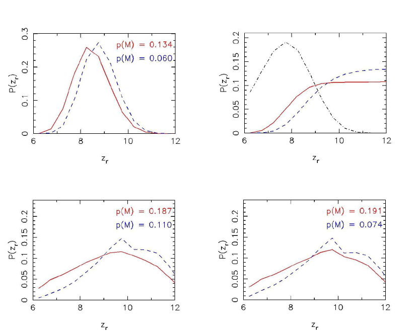
Figure 5: Constraints on reionisation redshift based on measured values of $T_{\rm 0}$, $\tau_{\rm CMB}$ and $\Gamma_{\rm-12}$ for different models of reionisation. In each case two probability distributions are shown, representing constraints from the fiducial near-zone temperature measurements of Bolton et  al. (2011) (red solid curves) and allowing for a larger Jeans scale (blue dashed curves). The relative probabilities of each model are shown in the top corner of each plot. Upper Left: Constraints from $T_{\rm 0}$ and $\tau_{\rm CMB}$ and the linear model for $N_{\rm ion}$. Upper Right: Constraints obtained from the near-zone temperatures and $N_{\rm ion}$ alone. For comparison, the constraint from $\tau_{\rm CMB}$ and $N_{\rm ion}$ alone is shown in black dot-dashed. Lower Left: The probability distributions for the cubic $N_{\rm ion}$ model. Lower Right: Distributions for the cubic model but now accounting for the bias of quasars to regions of high density.

In the upper panels of Figure 5, we present the resulting probability distribution functions over the parameter $z_{\rm r}$ for the linear $N_{\rm ion}$ model. The distributions are computed for the two different sets of measurements presented by Bolton et  al. (2011), derived from their fiducial model (red solid curves) and a model with additional pressure (Jeans) smoothing in the IGM (blue dashed curves). The latter effectively lowers the near-zone temperature constraints by $\sim 3000\rm\,K$. The upper left panel displays the $p(z_{\rm r})$ based on the measured values of $T_{0}$, $\tau_{\rm CMB}$ and $\Gamma_{-12}$. For comparison, in the upper right panel we also plot the individual distributions obtained by alternately considering constraints from either $\tau_{\rm CMB}$ or $T_{\rm 0}$ alone combined with our assumed $N_{\rm ion}$ evolution.

As expected, the measurement of $T_{\rm 0}$ alone does not differentiate between early reionisation redshifts, as for all scenarios the IGM has reached an asymptotic temperature. However, the temperature data do provide constraining power for low $z_{\rm r}$. We find that irrespective of which set of temperature measurements from Bolton et  al. (2011) is considered, very late reionisation is ruled out to high confidence. This is because the $5\,000{\rm K}$ increase in IGM temperature for $z_{\rm r}<6.5$, pushes the mean quasar temperature well above the observations.

In the lower panels of Figure 5 we show corresponding constraints for the cubic model excluding (lower left panel) and including (lower right panel) the effect of quasar density bias. In this model the observed value of $\tau_{\rm CMB}$ is used in defining the parameters governing $N_{\rm ion}$. It is therefore a much weaker a-posteriori constraint and we can no longer rule out reionisation at high redshift. Similarly for low $z_{\rm r}$, the smaller temperature differences between reionisation scenarios means that late reionisation cannot be excluded with the same confidence. Furthermore, the relatively tight constraints obtained when considering the temperatures derived assuming a larger Jeans scale are probably not robust, as the constraints from the fiducial measurements are favoured by a factor of around 3 over these.

The final model averaged distribution is shown in Figure 6, which corresponds to a mix of the fiducial results from the linear and cubic models. Even though this largely ignores the models with the tightest constraints, we may still conclude that $z_{\rm r}>7.9$ $(6.5)$ to 68 per cent (95 per cent) confidence. As a sanity check, we also verify that the optimal temperatures predicted by our reionisation models match the measurements quite well. Figure 7 shows the predicted sightline temperature distributions for the maximum a-posteriori estimates of $z_{\rm r}$ and $\alpha_{\rm q}^{\rm i}$ compared to the observed quasar temperatures. We find that although two thirds of the modelled points lie within the 68 per cent confidence intervals of the observations, the model temperatures of quasars 0 and 1 (following the numbering in Figure 7) appear to be systematically too high. However, for the fiducial Bolton et  al. (2011) measurements this does not provide a strong constraint ruling out our model, since the observed temperature distributions are both positively skewed and broader than Gaussian. Therefore, although our model predictions lie on the edge of the 68 per cent confidence interval, they are only about a factor of 1.5 less probable than the peak. The same does not hold true for the second set of measurements which account for additional Jeans smoothing. These are ruled out with some significance, which may be indicate that the (conservative) systematic error due to additional Jeans smoothing adopted by Bolton et  al. (2011) may have been slightly overestimated. The only real outlier then comes from quasar 5 in the fiducial measurements, which is unsurprising since this provides a significantly higher measurement of proximity-zone temperature. This may indicate that a quasar spectral index which is harder than the prior we have assumed (i.e. $\alpha_{\rm q}<1$) may be required to reconcile this measurement with the simulations.

It is interesting to contrast this result with recent evidence for a decline in the fraction of Lyman break galaxies which exhibit strong Ly$\alpha$ emission from $z=5$–$7$ (Ono et al., 2011; Pentericci et al., 2011; Schenker et al., 2011). Assuming the Ly$\alpha$ emission escape fraction does not evolve rapidly, this decline may be attributed to a corresponding decrease in the ionised hydrogen fraction to $Q\approx 0.5$ by $z=7$, implying reionisation finished late. In addition, analyses of the size and shape of the near-zone observed in the spectrum of the quasar ULAS J1120$+$0641 are consistent with $Q\leq 0.9$ at $z\simeq 7.1$ (Mortlock et al. 2011; Bolton et al. 2011), assuming the red damping wing is not due to a proximate high column density absorber. Large neutral fractions of $\sim 50$ per cent at $z\sim 7$ may be difficult to reconcile with our temperature measurements, which indicate $z_{\rm r}>7.9$ $(6.5)$ to 68 per cent (95 per cent). Such large neutral fractions could perhaps be reconciled with our constraint if the average quasar spectral index is much softer than we have assumed, resulting in lower temperatures for a given $z_{\rm r}$ due to less He$\,\rm\scriptstyle II\$photo-heating. On the other hand we note that other possible sources of hydrogen reionisation, such as population-III stars or mini-quasars, have harder spectra than we consider here. These would therefore tend to increase the heating immediately following reionisation. This would then drive IGM temperatures too high to match the Bolton et  al. (2011) observations assuming reionisation completed late. Consequently, sources which have harder spectra than we have assumed would strengthen rather than weaken our conclusion that late reionisation is unlikely.

Similar considerations also apply to uncertainties in the clumping factor $C$, briefly mentioned in Section 2.1. This is a highly uncertain parameter, whose impact we did not fully model but instead simply assumed to take on a uniform value of $C=3$. The clumping factor has an impact on temperature evolution, since increases in clumping factor tend to increase overall recombination, implying more photons are needed to achieve reionisation. This results in a corresponding increase in IGM heating on the order of $\sim 1\,000\rm K$ for $C=5$. However, we note that our choice of clumping factor lies at the low end of possible values derived from simulation (Pawlik et al. 2009; Raicević & Theuns 2011). Larger values of the clumping factor should then only rule out late reionisation with greater significance for models which have the same $z_{\rm r}$.

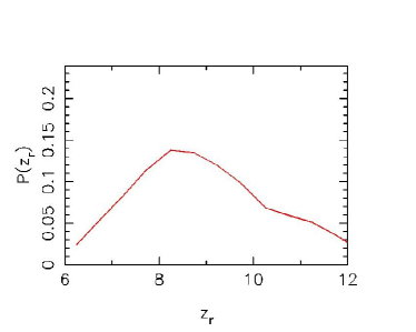
Figure 6: Final constraint on the reionisation redshift based on measured values of $T_{\rm 0}$, $\tau_{\rm CMB}$ and $\Gamma_{\rm-12}$ when averaged over all our different models of reionisation. This includes different models for $N_{\rm ion}$, the bias of quasars to high density regions and the Jeans pressure smoothing scale. Model averaging significantly weakens constraints as it adds uncertainties to the temperature, but still rules out late reionisation to $z_{\rm r}>7.9$ $(6.5)$ at 68 per cent confidence and 95 per cent confidence respectively.

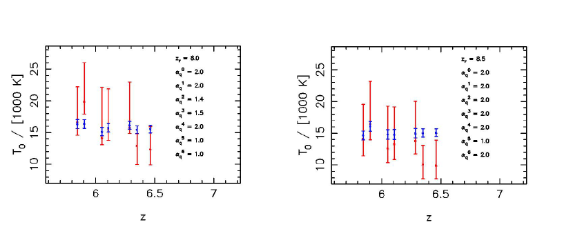
Figure 7: Model averaged quasar temperature distributions at the maximum a-posteriori estimate of reionisation redshift. We show both the model distributions (blue) and the observed sightlines (red) with 68 per cent confidence error bars. In both cases, we also include the parameter estimates of $z_{\rm r}$ and $\alpha_{\rm q}^{0}$ (rightmost point) through $\alpha_{\rm q}^{6}$ (leftmost point). For clarity, we omit redshift ranges and offset observations 3 and 5 by $\Delta z=0.1$. Left: Results obtained for the fiducial near-zone temperature measurements. Right: Results for the measurements with additional Jeans smoothing.

5.2 Prospects for constraints from future temperature measurements

In the previous section we presented constraints on the reionisation redshift from the existing measurements of the IGM temperature around quasars at $z\simeq 6$ (Bolton et  al. 2011). This work demonstrates the potential of high redshift IGM temperature measurements to aid in ruling out very late reionisation, so it is therefore interesting to consider if future progress can be made with further data.

We begin by creating mock catalogues of possible future observations. To do this, we assume that for a given $z_{\rm r}$, ionising source model and density bias model, $N_{\rm obs}$ observations are to be drawn. For each one, the quasar spectral index is drawn from the uniform prior over $\alpha_{\rm q}$ and the quasars are assumed to have an optically bright phase which starts at a redshift drawn from uniform distribution in the range $5.8<z<6.5$. The median of each new observation is taken at random from our predicted temperature distribution for the chosen $z_{\rm r}$, the redshift at which the quasar turns on and $\alpha_{\rm q}$. Finally, the errors in the measurement around this median are assumed to correspond to one of the 14 (7 fiducial and 7 augmented Jeans scale) observational measurements chosen at random. Once $N_{\rm obs}$ measurements are drawn in this way for each $z_{\rm r}$ and model, we then use equations (16) – (20) to obtain predicted probability distributions.

This procedure for the generation of mock observations is repeated 100 times, and the resulting distributions are averaged. We then marginalise over the different ionising source models to obtain a predicted distribution $p(z_{\rm r})$ for every $z_{\rm r}$ from which the measurements are drawn. This allows us to estimate the confidence with which the reionisation redshift can be measured as a function of the true $z_{\rm r}$. For simplicity, we omit the constraints imposed by ${\tau_{\rm CMB}}$ in order to assess the new information drawn from the temperature observations alone.

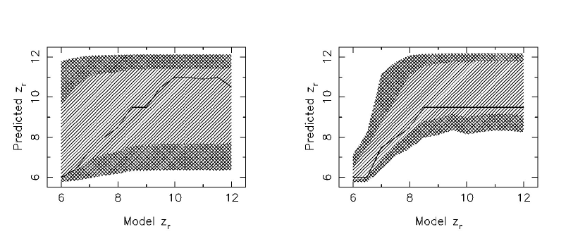
Figure 8: Bias and uncertainty in the constraints on the reionisation redshift from near-zone temperatures, as a function of the true reionisation redshift in our models. In each case the mode of the predicted posterior distribution is shown (black line) alongside the 68 per cent (lined region) and 95 per cent (hatched region) confidence intervals. Left: Results assuming 7 temperature measurements Right: Results for 100 near-zone temperature measurements, illustrating the optimistic case of large numbers of quasar sight-lines.

We present our results in Figure 8. The left panel shows the mode (solid line) and confidence intervals (filled regions) for $N_{\rm obs}=7$, mimicking the constraints of the previous section. Meanwhile, the right panel shows the same results for a large number of observations, $N_{\rm obs}=100$. We note that, in both cases, the mode typically recovers the true reionisation redshift in the models well, particularly for small $z_{\rm r}$. However, at no reionisation redshift do we obtain a particularly tight constraint for seven sight-lines only. For late reionisation, this is primarily due to uncertainties in modelling of both the quasar spectrum and the ionising efficiency. Similarly, if reionisation happened early, we will not be able to distinguish well between different $z_{\rm r}$ as the IGM temperature reaches an asymptotic state independent of when reionisation occurred. However, increasing the number of observations from 7 to 100 can tighten our constraints on late reionisation considerably, increasing the potential 95 per cent limit on $z_{\rm r}$ from 6.5 to 8.0.

Improved constraints the average quasar EUV spectra index from low redshift data could help to tighten our prior on $\alpha_{\rm q}$, and further improve limits at least on late reionisation. However, to tighten constraints on early reionisation using IGM temperature measurements ultimately requires observations which push to even higher redshifts.

6 Conclusions

Current understanding of the reionisation history is primarily built on existing observational evidence comprised of measurements of the Gunn-Peterson optical depth at $z\la 6$, and the electron scattering optical depth of cosmic microwave photons. These measurements respectively probe only the tail end of the epoch of reionisation, and an integral measure of the reionisation history. The available constraints therefore permit a wide range of possible histories. Observations of the IGM temperature provide an additional complementary probe since the thermal memory of the IGM yields information at redshifts beyond the those where observations are made. Measurements of the temperature around high redshift quasars therefore offer a renewed opportunity to constrain the reionisation history of the Universe.

In this paper, we have used measurements of IGM temperature at $z\simeq 6$ (Bolton et  al. 2011) to constrain the redshift at which the hydrogen reionisation epoch ended. Our analysis employs a semi-numerical model for reionisation and heating, which is constrained to fit the CMB electron scattering optical depth, and the ionisation rate inferred from the Ly$\alpha$ forest at $z=6$. We find that all models which reionise the Universe prior to $z_{\rm r}\approx 9.0$, settle to approximately the same IGM thermal state by $z=6.0$ with relatively little scatter in the temperature at mean density. For late reionisation, ($z_{\rm r}<8.0$), the situation is different since there is significantly more variance in the IGM temperature distribution. This arises partly from differences in ionisation time, which allow for different cooling times and a greater scatter. However, we find that there is always a detectable thermal imprint of at least $2\,500{\rm K}$, which differentiates the mean temperature signifying late reionisation $z_{\rm r}\approx 6$ from the asymptotic state achieved for $z_{\rm r}>9.0$. This implies that measurements of temperature in quasar near-zones can be used to constrain the reionisation redshift if it is sufficiently late.

Including observational constraints from the CMB electron scattering optical depth and the Ly$\alpha$ forest opacity, we conclude that $z_{\rm r}>7.9$ $(6.5)$ with 68 (95) per cent confidence. The $z\simeq 6$ temperature measurements therefore rule out a very late completion to reionisation. The inclusion of further temperature measurements in the future will tighten these constraints. If reionisation occurred early, we estimate a sample of 100 quasar spectra would rule out $z_{\rm r}<8.0$ to 95 per cent confidence. However, in order to push these constraints further, more detailed modelling of the IGM thermal evolution will also be required. In particular, the evolution of the ionising efficiency with redshift will have to be understood in order to narrow the modelling uncertainties for later reionisation scenarios. Including the effect of hydrogen reionisation sources which have harder spectra than we have assumed here will also be valuable. Finally, improved estimates of quasar spectral indices will aid in reducing uncertainties in the modelling of the near-zone temperatures.

References

- Anninos et al. (1997) Anninos P., Zhang Y., Abel T., Normal M. L., 1997, New Astronomy, 2, 209
- Barkana & Loeb (2001) Barkana R., Loeb A., 2001, Phys. Rep., 349, 125
- Becker et al. (2007) Becker G. D., Rauch M., Sargent W. L. W., 2007, ApJ, 662, 72
- Bond et al. (1991) Bond J. R., Cole S., Efstathiou G., Kaiser N., 1991, ApJ, 379, 440
- Bolton et al. (2005) Bolton J. S., Haehnelt M. G., Viel M., Springel V., 2005, MNRAS, 357, 1178
- Bolton et al. (2010) Bolton J. S., Becker G. D., Wyithe J. S. B., Haehnelt M. G., Sargent W. L. W., 2010, MNRAS, 406, 612
- Bolton et al. (2011) Bolton J. S., Becker G. D., Raskutti S., Wyithe J. S. B., Haehnelt M. G., Sargent W. L. W., 2011, MNRAS submitted
- Bolton & Haehnelt (2007) Bolton J. S., Haehnelt M. G., 2007, MNRAS, 374, 493
- Bolton et al. (2011) Bolton, J. S., Haehnelt, M. G., Warren, S. J., Hewett, P. C., Mortlock, D. J., Venemans, B. P., McMahon, R. G., & Simpson, C. 2011, MNRAS, 416, L70
- Bolton et al. (2004) Bolton, J., Meiksin, A., & White, M. 2004, MNRAS, 348, L43
- Bolton et al. (2009) Bolton, J. S., Oh, S. P., & Furlanetto, S. R. 2009, MNRAS, 395, 736
- Bromm et al. (2001) Bromm V., Kudritzki R. P., Loeb A., 2001, ApJ, 552, 464
- Carilli et al. (2010) Carilli, C. L. et al. 2010, ApJ, 714, 834
- Choudhury & Ferrara (2005) Choudhury T. R., Ferrara A., 2005, MNRAS, 361, 577
- Choudhury & Ferrara (2006) Choudhury T. R., Ferrara A., 2006, MNRAS, 371, L55
- Choudhury et al. (2009) Choudhury, T. R., Haehnelt, M. G., & Regan, J. 2009, MNRAS, 394, 960
- Coles & Jones (1991) Coles P., Jones B., 1991, MNRAS, 248, 1
- Dijkstra et al. (2004) Dijkstra M., Haiman Z., Rees M. J., Weinberg D. H., 2004, ApJ, 601, 666
- Dunkley et al. (2009) Dunkley J., et al., 2009, ApJS, 180, 306
- Eisenstein & Hu (1999) Eisenstein D. J., Hu W., 1999, ApJ, 511, 5
- Fan et al. (2006) Fan X., 2006, ApJ, 132, 117
- Faucher-Giguère et al. (2008) Faucher-Giguère, C.-A., Lidz, A., Hernquist, L., Zaldarriaga, M. 2008, ApJ, 688, 85
- Faucher-Giguère et al. (2009) Faucher-Giguère, C.-A., Lidz, A., Zaldarriaga, M., & Hernquist, L. 2009, ApJ, 703, 1416
- Furlanetto & Oh (2008) Furlanetto S. R., Oh S. P., 2009, ApJ, 681, 1
- Furlanetto & Oh (2009) Furlanetto S. R., Oh S. P., 2009, ApJ, 701, 94
- Geil & Wyithe (2008) Geil P. M., Wyithe J. S. B., 2008, MNRAS, 386, 1683
- Gnedin & Fan (2006) Gnedin N. Y., Fan X., 2006, ApJ, 648, 1
- Haiman & Loeb (1997) Haiman Z., Loeb A., 1997, ApJ, 483, 21
- Hu et al. (1995) Hu E. M., Kim T.-S., Cowie L. L., Songaila A., Rauch M. 1995, AJ, 110, 1526
- Hui & Gnedin (1997) Hui L., Gnedin N. Y., 1997, MNRAS, 292, 27
- Hui & Haiman (2003) Hui L., Haiman Z., 2003, ApJ, 596, 9
- Komatsu et al. (2009) Komatsu E., Dunkley J., Nolta M. R., et al., 2009, ApJS, 180, 330
- Komatsu et al. (2011) Komatsu E., Smith K. M., Dunkley J., et al., 2009, ApJS, 192, 18
- Leitherer et al. (1999) Leitherer C. et al., 1999, ApJS, 123, 3
- Lidz et al. (2007) Lidz A., McQuinn M., Zaldarriaga M., Hernquist L., Dutta S., 2007, ApJ, 670, 39
- Madau & Meiksin (1994) Madau P., Meiksin A., 1994, ApJ, 433, L53
- Mesinger (2010) Mesinger A., 2010, MNRAS, 407, 1328
- Mesinger & Furlanetto (2007) Mesinger, A. & Furlanetto, S. 2007, ApJ, 669, 663
- Miralda-Escudé (2003) Miralda-Escudé, J. 2003, ApJ, 597, 66
- Miralde-Escude & Rees (1994) Miralda-Escude J., Rees M. J., 1994, MNRAS, 266, 343
- Misawa et al. (2007) Misawa T., Tytler D., Iye M., Kirkman D., Suzuki N., Lubin D., Kashikawa N., 2007, AJ, 134, 1634
- Mitra et al. (2011) Mitra S., Choudhury T. R., Ferrara A., 2011, MNRAS, 413, 1569
- Mortlock et al. (2011) Mortlock, D. J. et al. 2011, Nature, 474, 616
- Ono et al. (2011) Ono, Y. et al. 2011, ApJ submitted, (arXiv:1107.3159)
- Pawlik et al. (2009) Pawlik A. H, Schaye J., & van Scherpenzeel E., 2009, MNRAS, 394, 1812
- Pentericci et al. (2011) Pentericci, L. et al. 2011, ApJ submitted, (arXiv:1107.1376)
- Petitjean et al. (1993) Petitjean P., Webb J. K., Rauch M., Carsell R. F., & Lanzetta K. M., 1993, MNRAS, 262, 499
- Pritchard et al. (2009) Pritchard J. R., Loeb A., Wyithe J. S. B., 2009, MNRAS, 408, 57
- Raicević & Theuns (2011) Raicević M., Theuns T., 2011, MNRAS, 412, L16
- Schenker et al. (2011) Schenker, M. A, et al. 2011, Submitted to ApJ, arXiv:1107.1261
- Sheth & Tormen (2002) Sheth R.K., Tormen G., 2002, MNRAS, 329, 61
- Songaila & Cowie (2010) Songaila A., Cowie L. L., 2010, ApJ, 721, 1448
- Telfer et al. (2002) Telfer, R. C., Zheng, W., Kriss, G. A., & Davidsen, A. F. 2002, ApJ, 565, 773
- Theuns et al. (2002) Theuns, T., Schaye, J., Zaroubi, S., Kim, T., Tzanavaris, P., & Carswell, B., 2002, ApJ, 567, L103
- Thomas et al. (2009) Thomas, R. M., Zaroubi, S., Ciardi, B., Pawlik, A. H., Labropoulos, P., Jelić, V., Bernardi, G., Brentjens, M. A., de Bruyn, A. G., Harker, G. J. A., Koopmans, L. V. E., Mellema, G., Pandey, V. N., Schaye, J., & Yatawatta, S. 2009, MNRAS, 393, 32
- Trac et al. (2008) Trac, H., Cen, R., & Loeb, A., 2008, ApJ, 689, L81
- Verner et al. (1996) Verner D. A., Ferland G. J., Korista K. T., Yakovlev D. G., 1996, ApJ, 465, 487
- White et al. (2003) White R., Becker R., Fan X., Strauss M., 2003, Astron J, 126, 1
- Wyithe & Bolton (2011) Wyithe J. S. B., Bolton J. S., 2011, MNRAS, 412, 1926
- Wyithe et al. (2010) Wyithe J. S. B, Hopkins A. M., Kistler M. D., Yuksel H., Beacom J. F., 2010, MNRAS, 401, 2561
- Wyithe & Loeb (2003) Wyithe J. S. B., Loeb A., 2003, ApJ, 586, 693
- Wyithe & Loeb (2007) Wyithe J. S. B., Loeb A., 2007, MNRAS, 375, 1034
- Wyithe & Morales (2007) Wyithe J. S. B., Morales M. F., 2007, MNRAS, 379, 1647
- Zahn et al. (2007) Zahn, O., Lidz, A., McQuinn, M., Dutta, S., Hernquist, L., Zaldarriaga, M., & Furlanetto, S. R. 2007, ApJ, 654, 12
- Zaldarriaga et al. (2001) Zaldarriaga M., Hui L., Tegmark M., 2001, ApJ, 557, 519