The Lyman $\alpha$ forest flux probability distribution at ${\boldmath z>3}$

Abstract

We present a measurement of the Lyman $\alpha$ flux probability distribution function (PDF) obtained from a set of eight high resolution quasar spectra with emission redshifts at $3.3\leq z\leq 3.8$. We carefully study the effect of metal absorption lines on the shape of the PDF. Metals have a larger impact on the PDF measurements at lower redshift, where there are relatively fewer Lyman $\alpha$ absorption lines. This may be explained by an increase in the number of metal lines which are blended with Lyman $\alpha$ absorption lines toward higher redshift, but may also be due to the presence of fewer metals in the intergalactic medium at earlier times. We also provide a new measurement of the redshift evolution of the effective optical depth, $\tau_{\rm eff}$, at $2.8\leq z\leq 3.6$, and find no evidence for a deviation from a power law evolution in the $\log(\tau_{\rm eff})-\log(1+z)$ plane. The flux PDF measurements are furthermore of interest for studies of the thermal state of the intergalactic medium (IGM) at $z\simeq 3$. By comparing the PDF to state-of-the-art cosmological hydrodynamical simulations, we place constraints on the temperature of the IGM and compare our results with previous measurements of the PDF at lower redshift. At redshift $z=3$, our new PDF measurements are consistent with an isothermal temperature-density relation, $T=T_{0}\Delta^{\gamma-1}$, with a temperature at the mean density of $T_{0}=19250\pm 4800$ K and a slope $\gamma=0.90\pm 0.21$(1$\sigma$ uncertainties). In comparison, joint constraints with existing lower redshift PDF measurements at $z<3$ favour an inverted temperature-density relation with $T_{0}=17900\pm 3500$ K and $\gamma=0.70\pm 0.12$, in broad agreement with previous analyses.

1 Introduction

The Lyman $\alpha$ forest corresponds to the large number of absorption features located blueward of the Lyman $\alpha$ emission line in the spectra of quasi-stellar objects (QSOs). In the last decade, thanks to the power of 10-m class telescopes equipped with high-resolution spectrographs, considerable progress has been made toward understanding the nature of these absorption features. This population of discrete lines is due to HI absorption arising from the filamentary structure of the cosmic-web, and in the approximation of a Gaussian velocity dispersion can be well described by a series of Voigt profiles (Rauch 1998). A variable amount of absorption in the Lyman $\alpha$ forest is also due to ultraviolet (UV) transitions from heavy element ions which are usually associated with strong Lyman $\alpha$ lines.

Quantities often studied in analyses of QSO spectra include the power spectrum of the flux distribution, which is used to constrain cosmological parameters and probe the dark matter power spectrum on scales of order of 50 $h^{-1}$ Mpc (e.g. Croft et al. 2002, Viel et al. 2004, McDonald et al. 2006). Another quantity thoroughly studied in the last few years is the flux probability distribution function (PDF), which is sensitive not only to the spatial distribution of dark matter, but also to the thermal state of the intergalactic medium (IGM). Previous studies of the Lyman $\alpha$ forest PDF have shed light on the physical state of the IGM mostly at $z<3$. Bolton et al. (2008) compared the flux PDF measured from a sample of QSO spectra presented by Kim et al. (2007, hereafter K07) to a set of hydrodynamical simulations of the Lyman $\alpha$ forest, exploring different cosmological parameters and various thermal histories. Agreement between the data and simulations was obtained by adopting a power-law temperature-density relation, $T=T_{0}\Delta^{\gamma-1}$ (Hui & Gnedin 1997), where the low density IGM ($\Delta=\rho/\langle\rho\rangle\leq 10$) was close to isothermal (i.e. with $\gamma\sim 1$) or inverted ($\gamma<1$). This result implied that the low-density regions of the IGM may be considerably hotter and their thermal state more complicated than usually assumed at these redshifts.

Radiative transfer effects during the epoch of HeII reionization, which should occur at $z>3$, are expected to play a non negligible role in setting this temperature-density relation. Indeed, evidence that the tail-end of HeII reionization is occurring at $z\simeq 3$ is supported by a variety of observations, such as the opacity of the HeII Lyman $\alpha$ forest (Reimers et al. 1997; Heap et al. 2000; Kriss et al. 2001, Shull et al. 2010, Worseck et al. 2011, Syphers et al. 2011), an increase in the temperature of the IGM at mean density toward $z\simeq 3$ (Schaye et al. 2000, Theuns et al. 2002, Lidz et al. 2010, Becker et al. 2011, but see McDonald et al. 2001, Zaldarriaga, Hui, & Tegmark 2001), the observed evolution of the CIV/SiIV metal-line ratio (Songaila & Cowie 1996; Songaila 1998, but see Kim, Cristiani & D’Odorico 2002) and the evolution of the Lyman $\alpha$ forest effective optical depth (Bernardi et al. 2003, Faucher-Giguere et al. 2008, Pâris et al. 2011, but see Bolton, Oh & Furlanetto 2009b).

However, recent work suggests that photo-heating during HeII reionization alone is not sufficient to achieve an inverted temperature-density relation, $\gamma<1$ (McQuinn et al. 2009; Bolton, Oh & Furlanetto 2009a). A recently proposed alternative channel for heating, which naturally produces an inverted temperature-density relation, may be provided by very energetic gamma rays from blazars (Chang et al 2011, Puchwein et al. 2011). In this scenario, very high energy gamma rays annihilate and pair produce on the extragalactic background light. Powerful plasma instabilities then dissipate the kinetic energy of the electron-positron pairs locally, volumetrically heating the IGM. On the other hand, continuum placement errors could partly explain the preference of the K07 data for an inverted temperature-density relation (see Lee 2012 for a recent discussion). Indeed, Bolton et al. (2008) and more recently Viel et al. (2009) found an isothermal temperature-density relation was consistent (within $1.5\sigma$) with the K07 PDF constraints when treating continuum uncertainties conservatively.

Ultimately, however, for further progress in understanding the origin of an inverted temperature-density relation, additional observational constraints on the IGM thermal state are required. An investigation of the flux probability distribution at redshifts around $z\sim 3$ or higher may therefore shed more light on the possible inversion of the temperature-density relation. Such a measurement is also complementary to other constraints on the IGM thermal state, such as those presented recently by Becker et al. (2011), where the temperature-density relation is not measured directly. Such an investigation is the main motivation of the present work.

In this paper, we use eight high resolution QSO spectra observed at $3.3\leq z\leq 3.8$ to extend the study of the Lyman $\alpha$ forest PDF by K07 to higher redshifts. The aim of this paper is two-fold. First, we perform a detailed study of the redshift evolution of the flux PDF across a wide redshift range. This enables us to study possible systematic trends in the PDF due to redshift-dependent effects, such as the presence of metal absorption lines. In order to corroborate our analysis, we also measure the Lyman $\alpha$ effective optical depth and compare it to different estimates by other authors. In the second step, the measured flux PDF is compared to theoretical results obtained from cosmological hydrodynamical simulations. This enables us to investigate the thermal state of the IGM during this interesting redshift range.

This paper is organized as follows. In Section 2, we present the QSO spectra and the data analysis, and in Section 3 we present our measurements of the flux PDF and effective optical depth. In Section 4, we introduce the hydrodynamical simulations used to obtain constraints on the thermal state of the IGM from the PDF and, in Section 5, we report the results from the analysis of the simulations. Finally, in Section 6, we present our conclusions.

2 The data set

The data set used in this paper consists of eight high-redshift QSO spectra. Two of the spectra (PKS2126-158 and PKS2000-330) were obtained with the Ultraviolet and Visual Echelle Spectrograph (UVES) (Dekker et al. 2000) at the Kueyen unit of the European Southern Observatory (ESO) VLT (Cerro Paranal, Chile) as part of the ESO Large Programme (LP): ‘The Cosmic Evolution of the IGM’ (Bergeron et al. 2004). PKS1937-101 is from the program Carswell et al. 077.A-0166(A), Q1317-0507, SDSSJ16212-0042 and Q1249-0159 are from Kim et al. 075.A-0464(A), Q1209+0919 is from the program Dessauges-Zavadsky et al. 073.B-0787(A) and Q0055-269 is from D’Odorico et al. 65.O-0296(A). All the spectra have been reduced with the standard UVES pipeline provided by ESO. Wavelengths have been corrected to vacuum-heliocentric.

Table 1: The QSO sample used in this work. In the first column the name of the QSO is reported. Subsequent columns list the emission redshift of the QSO, the redshift range covered by the Lyman $\alpha$ forest, the wavelength range covered by the Lyman $\alpha$ forest and the signal to noise (S/N, see text for details). Note the wavelength range of the Lyman $\alpha$ forest excludes the region 4000 km s^-1 bluewards of the Lyman $\alpha$ emission line in order to avoid the proximity effect (see Sect.2.2).

QSO	$z_{\rm em}$a	$z_{\rm Ly\alpha}$	$\lambda_{\rm Ly\alpha}$ (Å)	S/N	Notes
PKS2126-158	3.292	2.68-3.23	4473-5148	110	1 LLS ($z$=2.967),
					2 Sub-DLAs ($z$=2.638, 2.769)
Q1209+0919	3.295	2.62-3.23	4404-5150	25	8 LLS
Q0055-269	3.66	2.93-3.59	4775-5583	51
Q1249-0159	3.66	2.94-3.60	4784-5594	70	3 LLS ($z$=3.102, 3.5243, 3.5428)
SDSSJ16212-0042	3.70	2.97-3.63	4821-5637	93	2 LLS ($z$=3.106, 3.144)
Q1317-0507	3.71	2.98-3.66	4840-5659	86	1 LLS ($z$=3.288)
PKS2000-330	3.78	3.03-3.72	4903-5733	68	2 LLS ($z$=3.189, 3.33)
PKS1937-101	3.79	3.04-3.72	4910-5742	150

^a In some cases, the emission redshift $z_{\rm em}$ estimated on the basis of the QSO Lyman $\alpha$ emission line is an underestimation of the true value (see K07). If Lyman $\alpha$ absorption lines with $z>z_{\rm em}$ are present, we assume the highest redshift of the absorption line as a proxy for $z_{\rm em}$.

Figure 1: The eight QSO spectra which comprise our sample. Each spectrum is normalised to the quasar continuum and the wavelengths are displayed in the QSO rest-frame. For each QSO, the upper panel shows the normalised spectrum, whereas the lower panel displays all the spectral regions containing metal lines. To measure the PDF, these regions have been masked following the criteria described in Sect. 2.3. In each panel, the left dotted line and the right dotted line indicate the wavelengths of the Lyman $\beta$ and Lyman $\alpha$ transitions. The regions with no flux, such as the one apparent in the spectrum of PKS 2000-330 centered at $\lambda\sim 1180$ Å, are due to the wavelength gaps caused by using three separate CCDs in the dichroic setting.

The properties of the QSO spectra used in this paper are summarized in Table 1. The velocity resolution of each spectrum is 6.7 km s^-1 full-width half maximum, and each spectrum is binned in 0.05 Å  pixels. The signal-to-noise (S/N) ratio has been calculated by considering regions of the spectra redwards of the QSO emission peak, and corresponds to the inverse of the standard deviation of the average normalized flux for pixels free of absorption. For some QSOs, the spectra have already been used by D’Odorico et al. (2010) for the study of the evolution of CIV in the IGM. The spectra of three QSOs (Q1317-0507, Q1249-0159 and SDSSJ16212-0042) have been reduced for this work.

Most of the QSOs include one or more Lyman Limit systems (LLS), i.e. absorption systems with neutral column density $17.2\leq\log(N_{\rm HI}/{\rm cm}^{-2})\leq 19$. For the comparison of our data to simulation results, we have therefore excised all the pixels belonging to the spectral regions included in the range $\lambda_{\rm LLS}-50$ Å  $\leq\lambda\leq\lambda_{\rm LLS}+50$ Å, where $\lambda_{\rm LLS}$ is the central wavelength of the LLS. PKS2126-158 additionally includes two sub-damped Lyman $\alpha$ systems ($19\leq\log(N_{\rm HI}/{\rm cm}^{-2})\leq 20.3$). The spectral regions where these systems are present have also been excised from the spectrum, following the same criterion as for LLS. In addition, the identified metal lines associated with both LLS and sub-DLAs have been removed from the spectra as described in Sect. 2.3.

The two QSOs PKS2126−158 and Q0055-269 were also included in the K07 sample. It is worth noting that the wavelength ranges for PKS2126−158 and Q0055-269 used in this work are different to those reported in Tab. 1 of K07. In the case of PKS2126−158, our blue wavelength cut is different to the K07 value due to the presence of two sub-DLAs at $z=2.638$ and $z=2.769$. We excluded the two regions contaminated by the sub-DLAs as described above, and a small region between the two sub-DLAs was left in our spectrum, extending from 4470 Å  to 4540 Å. K07 instead decided to remove this region and cut their spectrum at 4630 Å. The red wavelength cut was chosen by K07 in order to avoid having pixels at wavelengths $>5112$ Å  corresponding to redshifts $z>3.2$. However, this redshift range is important for studying the possible effects of HeII reionization and so we include it in this work. In the case of Q0055-269, the blue cut was performed in our spectrum at a wavelength corresponding to the Lyman $\beta$ emission line, whereas in the case of K07 they performed it at $4785$ Å  in order to exclude a metal absorption system at 4784 Å. The red cut was performed by K07 at $5112$ Å  to again discard pixels with $z>3.2$.

In Fig. 1, we show the reduced spectra for all the QSOs of our sample and, for each spectrum, the contamination from metal lines. The regions containing metal lines have been masked following the criteria described in Sect. 2.3. In Fig. 2, for each QSO spectrum, the redshift coverage and the Lyman $\alpha$ forest wavelength coverage are shown.

Figure 2: The solid lines display the redshift (and wavelength, see upper axis) coverage of the Lyman $\alpha$ forest in the QSO spectra used in our sample. The dashed lines at $z=2.62$, $z=3.17$ and $z=3.72$ represent the extremes of the two redshift bins used to calculate the flux probability distribution function, as described in Sect. 3.

2.1 Continuum fitting

In each spectrum all the absorption lines redwards of the Lyman $\alpha$ emission line, as well as those belonging to the Lyman $\alpha$ forest, have been fitted with Voigt profiles. To satisfactorily perform this task, for each spectrum a precise estimate of the continuum is required. However, the problem of continuum fitting high resolution data requires particular attention, and it has been widely discussed in the literature (e.g. K07; Desjacques et al. 2007; Faucher-Giguere et al. 2008). An automatic procedure to fit QSO spectra has also been developed by Dall’Aglio et al. (2008a; 2008b). They used an extended sample of high resolution, high S/N QSO spectra, and by means of an adaptive techinque involving cubic spline interpolations and a Monte-Carlo method, they were able to estimate the QSO continua and relative uncertainties. In this paper, however, continuum fitting was performed on our smaller data set as described below. It will be interesting to use a larger sample in the future to develop automatic techniques for continuum fitting and investigate associated uncertainties further.

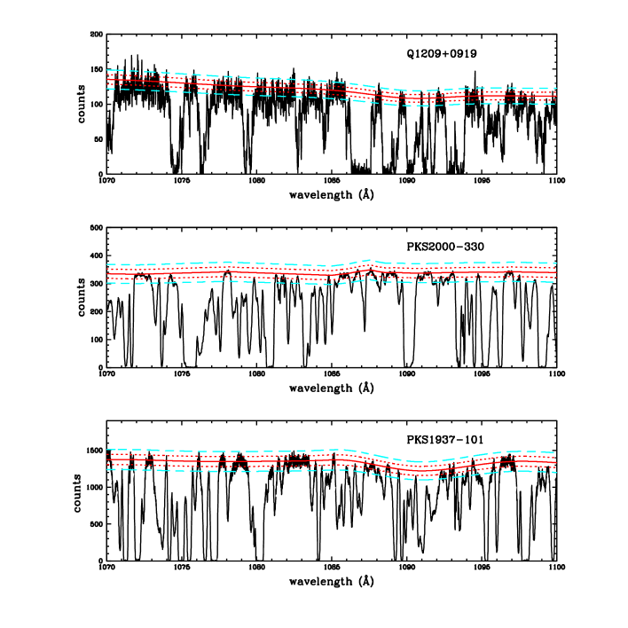
Figure 3: An illustration of the uncertainty on the continuum placement for three of the spectra in our sample with different S/N values: S/N=25 for Q1209+0919 (upper panel), S/N=68 for PKS2000-330 (middle panel) and S/N=150 for PKS1937-101 (lower panel). In each panel, the final continuum fit is shown by the solid curve, while the dotted and dashed curves show the fitted continuum after it is increased/decreased by 5 per cent and by 10 per cent, respectively.

For each QSO, the continuum was fitted using the IRAF package, by means of high-order polynomial functions. The continuum fitting was performed by cutting each spectrum into several chunks, depending on the S/N and on the number of absorption lines, and then joining the chunks back together into one single spectrum. The continua were determined by using regions free of absorption lines. This task does not present substantial difficulties when the region redwards of the QSO Lyman $\alpha$ emission line is considered, since this region presents only a few (metal) absorption lines. However, regions bluewards of the QSO Lyman $\alpha$ emission lines, such as the Lyman $\alpha$ forest, are instead populated by a large number of absorption lines. In general, the higher the emission redshift of the QSO, the greater the average Lyman $\alpha$ forest opacity. This makes continuum fitting toward higher redshift more difficult, since regions which are free of absorption lines become increasingly small and rare. In this case, a linear interpolation between two subsequent absorption-free chunks is used as a first-order guess for the continuum level. Another major problem in continuum fitting concerns the possible presence of wide and shallow absorption features in the spectra. Large-scale absorption can sometimes be incorrectly attributed to unabsorbed parts of the spectrum. This represents a problem in this procedure, since it can lead to an underestimate of the true continuum. To avoid such mistakes, it is necessary not only to check carefully every small chunk of the spectrum which is being fitted, but also the joint spectrum by searching for possible wide depressions due to large-scale absorption features which are not visible while working on the individual chunks. All the spectra and the fitted continua have been repeatedly and independently checked in this manner in order to identify such features and to avoid continuum underestimates.

As discussed in K07, the uncertainty on the continuum depends on the S/N, which varies not only from spectrum to spectrum, but may even vary within one single spectrum. As a general rule, the higher the S/N, the smaller the continuum uncertainty. This is illustrated in Fig. 3 where we show three unnormalized spectra with their final fitted continuum (solid lines), and with the continuum increased and decreased by 5 per cent (dotted lines) and by 10 per cent (dashed lines). The cases depicted in Fig. 3 represent the spectrum with the lowest S/N in Tab. 1 (Q1209+0919, upper panel), one case with an intermediate S/N value (PKS2000-330, middle panel) and the spectrum with the highest S/N (PKS1937-101, lower panel). Although it is very difficult to precisely quantify the uncertainty for the continuum determination, Fig. 3 demonstrates that, in the case of Q1209+0919, an uncertainty of the order of 10 per cent is exaggerated, but an uncertainty of 5 per cent seems plausible. As stressed earlier, this case represents the spectrum with the worst S/N in our sample. In the other two cases, it appears that a continuum which is decreased or increased by 5 per cent represents an underestimation and overestimation, respectively, of the actual continuum. For this reason, a typical uncertainty of 5 per cent should be regarded as conservative and representative of most of the spectra in our sample, in agreement with the analysis of K07 and the one of Dall’Aglio et al. (2008a). Later on, the effects of the continuum estimate on the flux PDF will be investigated in more detail.

2.2 Voigt Profile fitting

Once the continuum fitting was completed, in each spectrum, all the absorption features blueward of the QSO Lyman $\alpha$ emission line were then fitted with Voigt profiles. The aim of this procedure is to determine, for each absorption line, the redshift $z$, the Doppler parameter $b$ and the column density $N$ of the physical system giving rise to that absorption feature.

The Lyman $\alpha$ forest includes the spectral region between the wavelengths of the Lyman $\beta$ emission line, $\lambda_{\beta}=1025.72\,(1+z_{\rm QSO})$, and the wavelength corresponding to the Lyman $\alpha$ emission line, i.e. $\lambda_{\alpha}=1215.67\,(1+z_{\rm QSO})$. To avoid contamination from the QSO line-of-sight proximity effect, in each spectrum we excluded an interval of 4000 km s^-1 bluewards of the Lyman $\alpha$ emission line. All the absorption features were then identified and fitted by means of the RDGEN, VPFIT and VPGUESS packages.

Firstly, all the metal absorption lines redwards of the QSO Lyman $\alpha$ emission peak were identified and fitted. This task does not present significant difficulties, since the number of absorption lines in this spectral region is relatively low and lines due to different transitions are rarely blended. Secondly, the identification of heavy element absorption in the Lyman $\alpha$ forest was performed. This task requires more attention owing to the large amount Lyman $\alpha$ lines in this region and to the frequent presence of broad, saturated absorption features. In this spectral region, isolated metal lines are very rare. Most of the metal absorption lines are blended with Lyman $\alpha$ lines, complicating the precise identification of metal line profiles. A common technique to search for metal absorption in the Lyman $\alpha$ forest therefore employs the use of velocity width profiles. Once a strong transition is identified at wavelengths redward of the QSO Lyman $\alpha$ emission line, e.g. due to CIV or SiIV, associated ionic transitions such as SiII, SiIII, CII at the corresponding redshift and velocity profile can be searched for in the Lyman $\alpha$ forest.

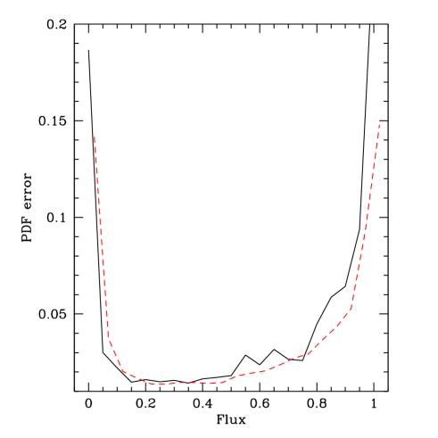
Figure 4: The flux PDF errors as a function of the normalised flux measured from all eight QSOs, computed by means of the jackknife (black solid lines) and the bootstrap (red dashed line) methods.

When metal lines in the Lyman $\alpha$ forest are heavily blended with HI absorption, it is generally difficult to identify the shape of the profile. The parameters which are most difficult to recover in this case are the Doppler parameter $b$ and the column density $N$. In these cases, as an initial guess for VPFIT we provide the profile of the lines associated with the systems already identified redwards of the QSO emission, usually satisfactorily fitted by VPFIT. VPFIT then corrects the initial guess and modifies it in order to obtain an improved fit to that spectral region. Once a stable solution is obtained which is not sensitive to the initial guess and characterised by a satisfactory reduced $\chi^{2}$ value (typically of the order of $1-3$, depending on the noise level of the spectrum) the fit process is complete. An alternative way to identify metal absorption in the forest is based on the value of the Doppler parameter, which is in general narrower than for Lyman $\alpha$ lines (e.g. Tescari et al. 2011). However, in this analysis any absorption not corresponding to an identified heavy element transition has been assumed to be due to Lyman $\alpha$ absorption.

2.3 Metal removal from the spectra

The presence of metal absorption alters the transmitted fraction in the QSO spectra and consequently the shape of the PDF. For this reason, in order to use the PDF as a probe of the physical state of the Lyman $\alpha$ forest, it is necessary to remove the metal absorption from the Lyman $\alpha$ forest in the QSO spectra.

Once the metal identification and Voigt profile fitting is complete, for each QSO we remove metal lines from the spectra in the following manner. The pixels belonging to spectral regions contaminated by identified metal absorption are excised from the spectra using a quantitative criterion which depends on the Doppler parameter of the metal absorption line, $b$. All the pixels at wavelengths, $\lambda$, within the interval $\lambda_{0}-\Delta\lambda\leq\lambda\leq\lambda_{0}+\Delta\lambda$ were removed from the spectra, where $\lambda_{0}$ is the central wavelength of the metal absorption line and $\Delta\lambda=\lambda_{Z,0}\,(1+z^{\prime})$. Here $\lambda_{Z,0}$ is the rest-frame wavelength of the transition of a given element $Z$ and $z^{\prime}=z-dz$, where $z$ is the redshift of the absorbing system and $dz=\frac{2\,b\sqrt{\ln\,2}\,(1+z)}{c}$. For each QSO spectra, we created a “mask” using this procedure, which is then used to remove the pixels belonging to the metal-contaminated regions.

The completeness of the masking is dependent on the success of identifying metals. It is clearly impossible to identify all the metal absorption in the Lyman $\alpha$ forest. In this work we are dealing with QSO spectra at $z>3$ which contain a large number of HI absorption lines. At these redshifts, metal lines are frequently blended with strongly saturated HI absorption, and when this is the case their contribution to the total absorption is negligible. However, there will be very few cases where the metal lines are isolated and not identified. For this reason, we believe that the results presented in this paper are not substantially affected by incomplete metal identification in the Lyman $\alpha$ forest. This issue will be discussed further in the section dedicated to the results.

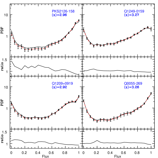
Figure 5: The effect of metal line absorption on the PDFs obtained for four of the QSOs in our sample. In the main panels, the solid curves display the PDFs calculated for each spectrum before removing metal lines. The solid squares with error bars show the PDFs calculated for the masked spectra, i.e. after removing the metal absorption. The dashed lines are drawn to guide the eye through the solid squares. For each QSO, the name and the average redshift of Lyman $\alpha$ forest absorption is indicated. In the smaller panels, the solid curve represents the ratio between the PDF calculated before and after removing metal lines.

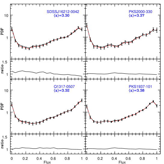
Figure 6: As in Fig.5, but now for the other four QSOs in our sample.

3 Data Analysis and results

Once each spectrum has been normalised to the continuum, i.e. once the quantity $F=S/C$ has been calculated for each pixel, where $S$ and $C$ are the observed flux and the estimated continuum, respectively, the flux probability distribution function can be measured. For each flux bin $F$, the PDF is calculated from the ratio between the number, $N_{\rm F,F+\Delta F}$, of pixels with flux between $F$ and $F+\Delta F$ and the total number, $N_{\rm tot}$, of pixels in the spectral region corresponding to the Lyman $\alpha$ forest (K07):

$${\rm PDF(F)}=\frac{N_{\rm F,F+\Delta F}}{N_{\rm tot}}.$$ (1)

The PDF is measured using this procedure in bins of width $\Delta F=0.05$ (McDonald et al. 2000; K07). We have assigned flux values $F=0$ and $F=1$ to all the pixels characterised by flux levels $F<0.025$ and $F>1$, respectively. The PDF is calculated both for single QSO spectra, and for the full sample. To study the redshift evolution of the PDF, we also divide the full sample in two redshift bins. The redshift bin width is chosen in order to have comparable numbers of pixels in each bin.

3.1 Error bar estimates

The error bars are estimated by means of a jackknife method, as described by Lidz et al. (2006). Once the PDF for a single QSO or for the full sample in a given redshift bin has been calculated, the contributing spectra are then divided into $n_{\rm c}$ chunks of width $\sim 50$ Å. If the PDF in the flux bin $F_{\rm i}$ is $\widehat{P}(F_{\rm i})$ and the PDF estimated without the $k$-th chunk in the flux bin $F_{\rm i}$ is $\widetilde{P}_{\rm k}(F_{\rm i})$, the covariance matrix cov$(i,j)$ between the PDF in flux bin $F_{\rm i}$ and the PDF in flux bin $F_{\rm j}$ can be defined as

$$\mathrm{cov}(i,j)=\sum_{k=1}^{n_{c}}[\widehat{P}(F_{i})-\widetilde{P}_{k}(F_{i})][\widehat{P}(F_{j})-\widetilde{P}_{k}(F_{j})],$$ (2)

For the flux bin $F_{\rm i}$, the errors computed with the jackknife method, $\sigma_{\rm J}$, are given by the square root of the diagonal of the matrix $\rm cov(i,j)$, i.e.

$$\sigma_{J}=\sqrt{\mathrm{cov(i,i)}}.$$ (3)

In addition, it is useful to have an alternative way to estimate the error bars for comparison to the uncertainties calculated using the jackknife method. We therefore also estimate error bars with a bootstrap technique. This technique consists of dividing the spectra into chunks of $\sim 5$ Å , and drawing a large number (500) of these chunks from the sample randomly with replacement. The PDF averaged over the 500 realizations coincides with the PDF of the random sample. For each flux bin, the uncertainty is then estimated by calculating the standard deviation of the PDFs obtained by sampling the 500 chunks with replacement.

In figure 4, the 1$\sigma$ errors for the PDF, estimated using the jackknife and bootstrap techniques, are compared. The PDF is computed from the full sample in this instance, without dividing the spectra into different redshift bins. Fig.  4 shows how the two methods provide comparable error estimates, although the jackknife estimates are larger at $F=0$ and $F=1$. In the remainder of the paper, unless otherwise stated, the uncertainties for the PDF will be computed by using the jackknife method.

Table 2: The mean PDF measured from the full sample, divided into two redshift bins and calculated by (1) using all pixels, (2) after removing contamination from metal absorption lines and (3) after removing Lyman limit systems and metal lines. Note that the redshift bins in the final two columns have a slightly different mean redshift due to the removal of LLS. The redshift bins have been slightly modified in order to have comparable numbers of pixels in each bin.

	All pixels		No metals		No metals, No LLS
	(1)		(2)		(3)
$F$	$<z>\,=2.90$	$<z>\,=3.45$	$<z>\,=2.90$	$<z>\,=3.45$	$<z>\,=2.95$	$<z>\,=3.48$
0.00	1.76 $\pm$ 0.18	2.37 $\pm$ 0.24	2.00 $\pm$ 0.16	2.38 $\pm$ 0.23	1.54 $\pm$ 0.11	2.28 $\pm$ 0.30
0.05	0.66 $\pm$ 0.05	0.71 $\pm$ 0.04	0.74 $\pm$ 0.04	0.72 $\pm$ 0.04	0.57 $\pm$ 0.04	0.70 $\pm$ 0.06
0.10	0.41 $\pm$ 0.03	0.41 $\pm$ 0.03	0.46 $\pm$ 0.03	0.43 $\pm$ 0.03	0.34 $\pm$ 0.03	0.42 $\pm$ 0.04
0.15	0.36 $\pm$ 0.02	0.34 $\pm$ 0.02	0.39 $\pm$ 0.02	0.36 $\pm$ 0.02	0.30 $\pm$ 0.03	0.35 $\pm$ 0.03
0.20	0.30 $\pm$ 0.01	0.33 $\pm$ 0.02	0.32 $\pm$ 0.01	0.35 $\pm$ 0.02	0.26 $\pm$ 0.02	0.35 $\pm$ 0.02
0.25	0.30 $\pm$ 0.02	0.33 $\pm$ 0.02	0.32 $\pm$ 0.02	0.34 $\pm$ 0.02	0.26 $\pm$ 0.03	0.35 $\pm$ 0.03
0.30	0.30 $\pm$ 0.02	0.36 $\pm$ 0.02	0.32 $\pm$ 0.02	0.37 $\pm$ 0.02	0.27 $\pm$ 0.02	0.36 $\pm$ 0.03
0.35	0.33 $\pm$ 0.02	0.35 $\pm$ 0.02	0.35 $\pm$ 0.02	0.36 $\pm$ 0.02	0.30 $\pm$ 0.02	0.35 $\pm$ 0.02
0.40	0.30 $\pm$ 0.02	0.37 $\pm$ 0.02	0.34 $\pm$ 0.02	0.38 $\pm$ 0.02	0.29 $\pm$ 0.03	0.36 $\pm$ 0.03
0.45	0.31 $\pm$ 0.01	0.41 $\pm$ 0.01	0.34 $\pm$ 0.01	0.42 $\pm$ 0.02	0.31 $\pm$ 0.02	0.42 $\pm$ 0.02
0.50	0.35 $\pm$ 0.02	0.46 $\pm$ 0.01	0.38 $\pm$ 0.02	0.47 $\pm$ 0.02	0.34 $\pm$ 0.02	0.48 $\pm$ 0.02
0.55	0.40 $\pm$ 0.02	0.58 $\pm$ 0.02	0.43 $\pm$ 0.02	0.58 $\pm$ 0.02	0.40 $\pm$ 0.04	0.60 $\pm$ 0.03
0.60	0.51 $\pm$ 0.02	0.61 $\pm$ 0.03	0.52 $\pm$ 0.02	0.62 $\pm$ 0.03	0.50 $\pm$ 0.03	0.62 $\pm$ 0.04
0.65	0.56 $\pm$ 0.02	0.71 $\pm$ 0.03	0.58 $\pm$ 0.02	0.72 $\pm$ 0.04	0.57 $\pm$ 0.03	0.72 $\pm$ 0.05
0.70	0.70 $\pm$ 0.04	0.81 $\pm$ 0.02	0.72 $\pm$ 0.04	0.82 $\pm$ 0.03	0.68 $\pm$ 0.03	0.84 $\pm$ 0.05
0.75	0.91 $\pm$ 0.05	0.95 $\pm$ 0.03	0.91 $\pm$ 0.05	0.96 $\pm$ 0.04	0.86 $\pm$ 0.04	0.97 $\pm$ 0.04
0.80	1.21 $\pm$ 0.05	1.13 $\pm$ 0.06	1.19 $\pm$ 0.05	1.14 $\pm$ 0.05	1.14 $\pm$ 0.05	1.15 $\pm$ 0.06
0.85	1.55 $\pm$ 0.06	1.37 $\pm$ 0.06	1.49 $\pm$ 0.06	1.38 $\pm$ 0.05	1.44 $\pm$ 0.07	1.40 $\pm$ 0.06
0.90	2.01 $\pm$ 0.09	1.88 $\pm$ 0.08	1.92 $\pm$ 0.08	1.87 $\pm$ 0.08	2.01 $\pm$ 0.10	1.93 $\pm$ 0.10
0.95	2.84 $\pm$ 0.07	2.66 $\pm$ 0.13	2.67 $\pm$ 0.07	2.56 $\pm$ 0.14	3.24 $\pm$ 0.12	2.69 $\pm$ 0.21
1.00	3.93 $\pm$ 0.19	2.89 $\pm$ 0.26	3.61 $\pm$ 0.18	2.77 $\pm$ 0.27	4.38 $\pm$ 0.29	2.69 $\pm$ 0.24

Table 3: The HI effective optical depth and its dependence on the contamination of metal absorption lines, calculated after dividing each spectrum in two redshift bins. In columns 1, 2 and 3 the name of the QSO, the Lyman $\alpha$ wavelength range and the average redshift are shown, respectively. In columns 4, 5 and 6 we report the HI effective optical depth with its error, the optical depth computed without removing metal lines with its error, and the percentage contribution of metal absorption, respectively.

QSO	wavelengths (Å)	$<\!z\!>$	$\tau_{\rm eff}$	$\tau_{\rm eff,HI+Z}$	$\tau_{\rm eff,HI+Z}$/$\tau_{\rm eff}$	metals (per cent)
PKS2126-158	4470-4880	2.85	0.329 $\pm$ 0.037	0.421 $\pm$ 0.041	1.278 $\pm$ 0.190	28
	4880-5148	3.12	0.238 $\pm$ 0.031	0.271 $\pm$ 0.031	1.138 $\pm$ 0.197	14
Q1209+0919	4404-4780	2.78	0.373 $\pm$ 0.031	0.423 $\pm$ 0.037	1.132 $\pm$ 0.136	13
	4780-5150	3.08	0.425 $\pm$ 0.040	0.450 $\pm$ 0.039	1.060 $\pm$ 0.135	6
Q0055-269	4774-5170	3.09	0.339 $\pm$ 0.033	0.344 $\pm$ 0.032	1.014 $\pm$ 0.137	1
	5170-5583	3.42	0.429 $\pm$ 0.036	0.439 $\pm$ 0.035	1.024 $\pm$ 0.119	2
Q1249-0159	4784-5190	3.10	0.382 $\pm$ 0.028	0.399 $\pm$ 0.028	1.045 $\pm$ 0.106	4
	5190-5594	3.44	0.529 $\pm$ 0.041	0.542 $\pm$ 0.040	1.024 $\pm$ 0.110	2
SDSSJ16212-0042	4821-5235	3.14	0.555 $\pm$ 0.042	0.596 $\pm$ 0.044	1.073 $\pm$ 0.113	7
	5230-5637	3.47	0.394 $\pm$ 0.032	0.427 $\pm$ 0.034	1.085 $\pm$ 0.123	8
Q1317-0507	4840-5240	3.15	0.384 $\pm$ 0.031	0.388 $\pm$ 0.031	1.010 $\pm$ 0.116	1
	5240-5659	3.48	0.495 $\pm$ 0.038	0.499 $\pm$ 0.039	1.008 $\pm$ 0.110	1
PKS2000-330	4903-5270	3.18	0.574 $\pm$ 0.048	0.582 $\pm$ 0.046	1.015 $\pm$ 0.117	1
	5270-5734	3.53	0.553 $\pm$ 0.043	0.570 $\pm$ 0.041	1.029 $\pm$ 0.108	3
PKS1937-101	4910-5323	3.21	0.371 $\pm$ 0.027	0.376 $\pm$ 0.027	1.014 $\pm$ 0.103	1
	5323-5742	3.55	0.487 $\pm$ 0.037	0.492 $\pm$ 0.036	1.011 $\pm$ 0.106	1

3.2 The effect of the metals

The effect of metal absorption on the PDF is displayed in Figures 5 and 6, where we show the PDF obtained from each of the eight QSOs in our sample. In these two figures, the solid and dashed curves in the large panels show the PDF computed including and excluding metal absorption lines, respectively. In the small panels, for each QSO the ratio between the PDF calculated including metals and after removing the metals is shown. The average Lyman $\alpha$ forest redshift spans from 2.96, for PKS2126-158, up to 3.38 in the case of PKS1937-101.

In general, the effect of removing metals on the PDF is to decrease the number of pixels with low flux and increase the number of pixels with high flux. As a result, the PDF computed after metal removal is slightly steeper than the PDF calculated before removing the metal absorption. This effect is most clearly visible for some of the QSOs in Fig. 5, such as PKS2126-158. For this spectrum, the effect of metal removal on the PDF is visible for flux values $F<0.6$, and is in agreement with the lower redshift analysis of K07, who find a PDF ratio similar to ours.

The effect of metal absorption on the PDF is also expected to depend on the redshift of the QSO and hence the average redshift of the Lyman $\alpha$ absorption. The impact of metal absorption on the PDF is expected to be more significant at lower redshifts, where Lyman $\alpha$ forest opacity is generally lower (K07). A weak trend with redshift is indeed visible in Figs. 5-6, but it is illustrated more clearly in Fig. 7, where for each QSO we show the ratio between the PDF calculated including metal lines and the PDF computed after removing metals from the spectra. The ratio is higher than 1.2 for flux values $F<0.4$ and lower than 0.9 for $F>0.9$ only in one case, PKS2126-158, which is one of the QSOs with the lowest value of $\langle z\rangle$ . Q1209+0919 has a comparable $\langle z\rangle$ and has a ratio close to 1.2 at $F<0.1$. The other six QSOs have similar $\langle z\rangle$ (between 3.26 and 3.38), and also exhibit comparable levels of metal contamination. For these six QSOs small fluctuations from one LOS to another are apparent, but the ratios are all between 0.9 and 1.2 and are much smaller than the variations for the QSOs at $\langle z\rangle<3$.

The redshift dependence of metal absorption may be understood in terms of the larger number of Lyman $\alpha$ absorption lines toward higher redshift, which leave less room for isolated metal absorption features. This does not necessarily mean that QSOs at higher redshifts have less metal absorption systems along their LOS, as the metal lines may instead be blended with Lyman $\alpha$ absorption lines. At the same time, however, this observation does not fully rule out the possibility the metal content of the intergalactic medium is decreasing toward higher redshift. We will return to the issue of metal contamination of QSO spectra in Sect. 3.5.

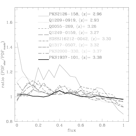
Figure 7: The ratios between the PDFs measured for each of the eight QSO spectra analysed in this work before and after the removal of metal line absorption. Note that the line thickness increases with the average Lyman $\alpha$ forest redshift.

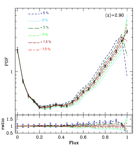
Figure 8: The effect of continuum placement uncertainty on the PDF calculated for our full sample in the lower redshift bin. In the upper panel, the solid line is the PDF calculated with the final continuum. The solid squares with error bars are the PDF values in each flux bin with the associated error estimated by means of the jackknife method described in Sect. 3.1. The short-dashed line, the long-dashed line and the dot-long-dashed line represent the PDF calculated by increasing the continuum level by 5, 3 and 1.5 per cent, respectively. The dotted line, the dot-short-dashed line and the short-dashed-long-dashed line represent the PDF calculated by decreasing the continuum level by 5, 3 and 1.5 per cent, respectively. In the lower panel, and following the same legend as above, the various lines display the ratio between the PDF calculated by increasing or decreasing the continuum and the PDF calculated with the final continuum. The errors on the ratios in the lower panel are similar for all curves but plotted only once for clarity.

3.3 The effect of the continuum uncertainty

The effects of the systematic uncertainty due to the continuum fitting procedure are shown in Fig. 8 for the full sample in the redshift bin centered at $z=2.9$. In this figure, the PDF is measured without removing the metal lines and is shown for the final continuum level (solid curve), as well as the PDF obtained by increasing and decreasing the continuum level by 5 per cent (dashed and dotted curves, respectively). Here the continuum is conservatively rescaled by 5 per cent since we have seen from Fig. 3 this value is representative of the continuum uncertainty for most of the spectra in our sample. In both cases, the strongest effects on the PDF are visible at high flux values ($F>0.5$), whereas a rescaling of the continuum has a negligible effect in the lowest flux bins.

The net effect of increasing the continuum by 5 per cent is to remove pixels at $F\sim 1$, moving the peak of the original PDF to lower flux bins. The bins at values $F<0.9$ are also populated with more pixels than is the case for the final continuum, and the slope of the PDF between $F\sim 0.1$ and $F\sim 0.9$ tends to increase overall. On the other hand, by decreasing the continuum by 5 per cent, pixels are instead moved towards higher flux bins and the PDF peaks at $F=1$.

The determination of the continuum is a very problematic task and subject to several uncertainties. However, Fig. 8 shows how the PDF would vary if we had systematically underestimated or overestimated the continuum by 5 per cent for all absorption systems. This seems rather implausible: it is far more likely that our continuum fitting method underestimates or overestimates the true continuum in chunks of our spectra, rather than consistently across the entire data set. If this is the case, the effect of the continuum placement on the PDF will be local (i.e. it should cause small variations around particular flux values), and will not affect its global average as strongly as Fig. 8 suggests. Regardless, however, when we turn to obtaining constraints on the thermal state of the IGM from our PDF measurements later, we follow Bolton et al. (2008) and Viel, Bolton & Haehnelt (2009) and only consider the PDF in the flux range $F=[0.1$–$0.8]$. This ignores the part of the PDF which is the most sensitive to continuum uncertainties, $F>0.8$.

3.4 Redshift evolution of the PDF

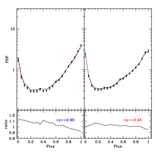
Figure 9: The redshift evolution of the PDF with the full sample divided into two redshift bins, $\langle z\rangle=2.90$ (left panels) and $\langle z\rangle=3.45$ (right panels). Upper panels: The squares with error bars represent the PDF measured after removing the metal line absorption. The dashed lines join the squares and are drawn in order to guide the eye. The solid lines are the PDFs computed for the full sample, but including metal absorption lines. Lower panels: The ratios between PDF calculated before and after removing the metal lines.

Fig. 9 shows the PDF computed for the full sample, divided into two different redshift bins, centered at redshifts 2.90 and 3.45. This figure also illustrates the effect of metal absorption lines on the PDF. The ratio between the PDF computed before and after removing metal absorption lines depends weakly on redshift.

The PDF for the full sample, divided into two redshift bins, is provided in Table 2. We tabulate the PDF computed for (1) all pixels, (2) after removing contamination from metal absorption lines and (3) after removing both metal absorption lines and Lyman limit systems; the latter has been used for the comparison with simulation results as described in Sect. 4. In Fig. 10, the PDFs excluding metals are compared to the PDFs obtained by K07 at lower redshift. For purposes of clarity, and to better focus on the evolution of the PDF, here the error bars are omitted. As already noted, the spectra at higher redshift are characterised by lower average flux levels. In terms of the PDF, this translates into a greater number of pixels with a low fluxes, resulting in a shallower distribution toward higher redshift. This trend is clearly visible in Fig.10.

It is also worth noting that a different method to remove metal absorption lines was used by K07. In the work of K07, pixels belonging to spectral regions including metals were not excised. The PDF was instead calculated by using the spectra fitted with VPFIT, including only Lyman $\alpha$ absorption lines. The use of these different methods could cause small differences between the PDFs. However, we have checked that these differences are within the error bars estimated with the jackknife method, and the results shown in Fig. 10 are unlikely to be significantly affected by the different methods used to remove metals from the QSO spectra.

Figure 10: The PDF measured in this work at $\langle z\rangle=2.9$ (squares and long-dashed line), $\langle z\rangle=3.45$ (circles and short-dashed line) compared with the PDF obtained by Kim et al. (2007) at $\langle z\rangle=2.07$ (light grey), $\langle z\rangle=2.52$ (grey) and $\langle z\rangle=2.94$ (dark grey).

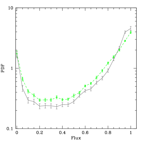
Figure 11: The PDF measured in this work in the lowest redshift bin (squares and long-dashed curve) plotted with error bars compared to the PDF obtained by Kim et al. (2007) at $\langle z\rangle=2.94$ (dark grey curve).

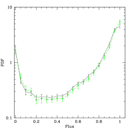
Figure 12: The flux PDF measured by K07 at $\langle z\rangle=2.94$ (dark grey curve) plotted with error bars compared to the PDF measured from the two spectra in our sample, Q0055-269 and PKS2126-158, used in the K07 measurement (open squares and long dashed curve). This comparison uses pixels in the same wavelength range adopted K07.

In addition, in Fig. 10 there is a difference between our PDF measured in the lowest redshift bin and the PDF obtained by K07 in their highest redshift bin, i.e. at $\langle z\rangle=2.94$. This difference is better illustrated in Fig 11, where we report our PDF calculated at $\langle z\rangle=2.90$ and the PDF measured by K07 at $\langle z\rangle=2.94$. Our PDF is higher than the K07 measurement by a factor ranging from 1.1 to 1.5 in the flux range $0.05\leq F\leq 0.8$. Note that two of the QSO spectra used in this study were also used in the PDF measurements presented by K07 (Q0055-269 and PKS2126-158). These objects contribute significantly to the highest bin of K07, as well as to our lowest redshift bin. As a sanity check, we have re-calculated the PDF with the two spectra of Q0055-269 and PKS2126-158 only, by using the pixels in the same wavelength range adopted by K07. The results of this test are visible in Fig. 12, along with jackknife error bars: once the same wavelength ranges as those of K07 for Q0055-269 and PKS2126-158 are taken into account, the two PDFs are consistent with each other within the uncertainties. This result tells us that the discrepancy between our PDF and K07’s is not due to a mistake in the computation of the PDF.

Since we expect that the flux PDF in a given redshift range does not depend on the sample of QSO spectra used to compute it, the observed discrepancy could be due to the modest size of the sample. If this is the case, our result should be more representative of the true value of the PDF since the sum of the $\Delta z$ of our QSO spectra contributing to the considered bin is larger than $\sim$ 50 per cent with respect to K07. We note also that the average redshift of the pixels belonging to our lowest redshift bin is larger than the corresponding value for K07’s highest redshift bin ($\langle z_{pixel}\rangle=3.03$ versus 2.91, respectively). This difference could contribute to the fact that, as seen in Fig.10, our PDF at $\langle z\rangle=2.90$ is higher than K07’s PDF at at $\langle z\rangle=2.94$.

Summarizing, while the evolution with redshift of the flux PDF is evident from Fig.10, more observations of QSOs at $z\sim 3.3$ could be needed to establish the true level of the flux PDF at $z\sim 2.9$.

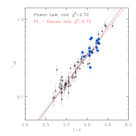
Figure 13: The redshift evolution of the Lyman $\alpha$ forest effective optical depth. The solid circles are the measurements from the present work. The triangles are the data from Schaye et al. (2003) and the diamonds are from Kim et al. (2007). The dashed line is the best fit power-law and the solid line the power-law plus Gaussian which best fits the whole sample of data (see text for details). The dotted line is the best fit power-law plus Gaussian obtained by Faucher-Giguere et al. (2008) from the study of a sample of high-resolution spectra.

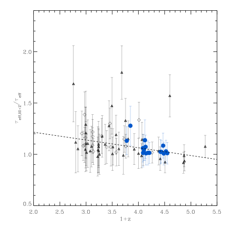
Figure 14: Redshift evolution of the ratio between the optical depth computed without removing the metal absorption and after the removal of the metal lines. The solid circles are the values computed in the present work. The triangles are the data by Schaye et al. (2003) and the diamonds are the data by Kim et al. (2007). The dashed line represents a straight-line fit to the data, $y=a\,x+b$, with $a=1.37$ and $b=-0.076$.

3.5 Redshift evolution of the HI optical depth

A quantity of interest in cosmology is the effective optical depth of the Lyman $\alpha$ forest, which is also sensitive to the thermal and ionization state of the IGM at high redshift. If $\langle F\rangle_{\rm HI}=\exp\left(-\tau_{\rm eff}\right)$ represents the average normalized flux measured from the Lyman $\alpha$ forest, the effective optical depth may be defined as $\tau_{\rm eff}\equiv-\ln\langle F\rangle_{\rm HI}$. The effective optical depth is therefore related to the average flux in all pixels in the Lyman $\alpha$ forest, and provides different and complementary measure to the PDF, which is a differential measurement.

In order to better probe the redshift range investigated in this paper and to increase the amount of information which can be extracted from our sample, we have divided each of the eight spectra analysed in this work into two redshift bins. In each bin we have then calculated the effective optical depth. In Tab. 3, we show the effective optical depth for our sample, computed both before and after removing metal contamination. We have calculated $\tau_{\rm eff}$ by considering the flux in the wavelength ranges reported in Tab. 3, after removing a fraction of pixels as described in section 2.2 in order to avoid the proximity effect. Note also that since we wish to measure the HI effective optical depth, removing metal lines is again very important for obtaining a precise estimate of $\tau_{\rm eff}$ which can be compared to other sets of data or with simulations.

The errors on $\tau_{\rm eff}$ are computed by means of a bootstrap method, as described in McDonald et al. (2000), Schaye et al. (2003) and K07. We have divided each spectrum into $N$ chunks of 100 pixels, corresponding to $5$ Å. A total of 500 bootstrap realizations were then performed by randomly selecting the $N$ chunks with replacement. The standard deviation from the mean $\tau_{\rm eff}$ is the error reported in Tab. 3. In the last column of Tab. 3 we also give the percentage contribution of metal absorption lines to $\tau_{\rm eff}$, which can be calculated as:

$${\mathrm{m}etals~{}(per~{}cent)}=(\frac{\tau_{\rm eff,HI+Z}}{\tau_{\rm eff}}-1)\cdot 100.$$ (4)

The metal contamination varies from 1 to 28 per cent; we will discuss its redshift dependence in more detail later on in this section.

In Fig. 13, we show the evolution of Lyman $\alpha$ forest optical depth, $\tau_{\rm eff}$, measured in this work after the removal of metal lines, compared to previous estimates by various authors. The dotted line is the best fit obtained by Faucher-Giguere et al. (2008) from a sample of 86 high-resolution, high-S/N ESI and HIRES quasar spectra. These authors also find evidence for a deviation of $\tau_{\rm eff}$ from a power-law at $z\sim 3.2$, consistent with the previous result of Bernardi et al. (2003) obtained using SDSS data and a different methodology (see also Pâris et al. 2011). The solid line is our best fit to all of the data (i.e. those of Schaye et al. 2003, Kim et al. 2007 and the present work) obtained by means of the relation

$$\tau_{\rm eff}=A(1+z)^{B}+C\exp\{-\frac{[(1+z)-D]^{2}}{2E^{2}}\},$$ (5)

which is a modified power-law including a Gaussian component to take into account the presence of a deviation, as in Faucher-Giguere et al. (2008). In comparison, the dashed line represents the best fit to the whole data ensemble for a power-law only. The reduced $\chi^{2}$ are reported in Fig. 13; we find that a power law provides a better fit to the data. In the case of a power law plus Gaussian, the best fit was obtained with $A=0.0023,B=3.64,C=-0.05,D=4.36,E=0.21$, i.e. with parameters associated with a very tiny deviation from a power law. Note also that the reduced $\chi^{2}$ reported in Fig  13 are in general larger than the values reported in table 5 of Faucher-Giguere et al. (2008). However, the data used by Faucher-Giguere et al. (2008) are more homogeneous and show a lower dispersion, hence it seems reasonable for their fits to show lower $\chi^{2}$ values. From these results, we conclude that, from our study of the redshift evolution of the effective optical depth, we do not find any strong evidence for a deviation from a power law. The best fit is expressed by the power law $\tau_{\rm eff}=0.0028\pm 0.0003\,(1+z)^{3.45\pm 0.08}$, in very good agreement with the previous best fit provided by K07: $\tau_{\rm eff}=0.0023\pm 0.0007(1+z)^{3.65\pm 0.21}$.

In Fig. 14, we show the redshift evolution of the ratio between the effective optical depth measured before and after removing metal absorption lines. This plot illustrates the effect of metal absorption on the Lyman $\alpha$ forest effective optical depth as a function of redshift. Our data are plotted together with the measurements from K07 and Schaye et al. (2003). The dashed line represents a straight-line fit to the data, $y=a\,x+b$. Our best fit values are $a=1.36$ and $b=-0.07$. The weak correlation shown in Fig. 14 again highlights the previously discussed redshift dependence of the metal line contamination in the Lyman $\alpha$ forest, which is consistent with a greater amount of metal absorption toward lower redshift.

4 The simulations

In this section, we now turn to describe the suite of hydrodynamic simulations used to obtain constraints on the thermal state of the IGM at redshift $z\,{}^{>}_{\rm\sim}\,3$ from our PDF measurements. Although the basic setup of the simulations is similar to earlier work by Bolton et al. (2008) and Viel et al. (2009), we now use new, higher resolution runs to explore a wider thermal history parameter space compared with those used by Viel et al. (2009). The simulations were performed using the parallel Tree-PM smoothed particle hydrodynamics (SPH) GADGET-2 code (Springel 2005) and its recently updated version GADGET-3. All the simulations were started at $z=99$, with initial conditions generated using the transfer function of Eisenstein & Hu (1999). The gravitational softening length was chosen to be equal to 1/30th of the mean linear interparticle spacing and star formation was included using a simplified prescription which converts all gas particles with temperature $T<10^{5}$ K and overdensity $\Delta=\rho/\langle\rho\rangle>10^{3}$ into collisionless stars.

Table 4: Summary of the hydrodynamical simulations used in this work. Column 1, simulation name: note the distinction between subset A (high resolution set) and the subset B (low resolution set); column 2, number of gas particles; column 3, mass of each gas particle; column 4, matter density parameter. In all models we assume a flat universe with $\Omega_{\rm\Lambda}=1-\Omega_{\rm 0m}$. However, $\Omega_{\rm b}h^{2}=0.023$ for the subset $A$ and $\Omega_{\rm b}h^{2}=0.024$ for the subset $B$ of our simulations; column 5, primordial power spectrum index; column 6, Hubble constant; column 7, fluctuation amplitude at a scale of 8 $h^{-1}$ Mpc; column 8, slope of the temperature-density ($T-\Delta$) relation, where $T(\Delta)=T_{\rm 0}\,\Delta^{\gamma-1}$; column 9: gas temperature at the mean density, in units of $10^{3}$ K, at $z=3.25$; column 10: further details on the simulations.

	Run	$N_{\rm GAS}$	$m_{\rm GAS}$	$\Omega_{\rm 0m}$	$n_{\rm s}$	$H_{\rm 0}$	$\sigma_{\rm 8}$	$\gamma$	$T_{\rm 0}$ ($10^{3}$ K)	Notes
			($h^{-1}$) M⊙			(km/s/Mpc)			($z=3.25$)
	A1REF	$512^{3}$	$9.2\times 10^{4}$	0.26	0.96	72	0.80	1.0	19.42	Fiducial high res. model
	A1CLD	$512^{3}$	$9.2\times 10^{4}$	0.26	0.96	72	0.80	1.0	14.93	Cold run
	A1HOT	$512^{3}$	$9.2\times 10^{4}$	0.26	0.96	72	0.80	1.0	23.88	Hot run
	A1LWγ	$512^{3}$	$9.2\times 10^{4}$	0.26	0.96	72	0.80	0.7	19.96	Low $\gamma$
	A1HIγ	$512^{3}$	$9.2\times 10^{4}$	0.26	0.96	72	0.80	1.3	19.07	High $\gamma$
	B1REF	$256^{3}$	$7.4\times 10^{5}$	0.26	0.95	72	0.85	1.0	23.79	Low res. reference model
	B1LS8	$256^{3}$	$7.4\times 10^{5}$	0.26	0.95	72	0.80	1.0	23.64	Low $\sigma_{\rm 8}$
	B1HS8	$256^{3}$	$7.4\times 10^{5}$	0.26	0.95	72	0.90	1.0	23.95	High $\sigma_{\rm 8}$
	B1LNs	$256^{3}$	$7.4\times 10^{5}$	0.26	0.90	72	0.85	1.0	23.67	Low $n_{\rm s}$
	B1HNs	$256^{3}$	$7.4\times 10^{5}$	0.26	1.00	72	0.85	1.0	23.93	High $n_{\rm s}$
	B1LOm	$256^{3}$	$7.4\times 10^{5}$	0.22	0.95	72	0.85	1.0	24.55	Low $\Omega_{\rm 0m}$
	B1HOm	$256^{3}$	$7.4\times 10^{5}$	0.30	0.95	72	0.85	1.0	23.12	High $\Omega_{\rm 0m}$
	B1LH0	$256^{3}$	$7.4\times 10^{5}$	0.26	0.95	64	0.85	1.0	25.40	Low $H_{\rm 0}$
	B1HH0	$256^{3}$	$7.4\times 10^{5}$	0.26	0.95	80	0.85	1.0	22.35	High $H_{\rm 0}$

In Table 4 we summarize the parameters used in the cosmological simulations. We use two different sets of simulations. Set A includes high resolution runs and, among them, the fiducial run for this paper: A1_REF. Each simulation has a box size of 10 $h^{-1}$ Mpc comoving and contains 2 $\times$ 512³ dark matter and gas particles. The model chosen is a flat $\Lambda$CDM cosmology with parameters: $\Omega_{\rm 0m}=0.26$, $\Omega_{\rm\Lambda}=0.74$, $\Omega_{\rm b}h^{2}=0.023$, $n_{\rm s}=0.96$, $H_{\rm 0}=72$ km s^-1 Mpc^-1 and $\sigma_{\rm 8}=0.80$, which are in agreement with recent studies of the cosmic microwave background (Komatsu et al. 2009; Reichardt et al. 2009; Jarosik et al. 2011).

We use set A to explore variations in the thermal state of the gas. A spatially uniform ultra-violet background (UVB) produced by quasars and galaxies (Haardt & Madau 2001) was adopted, where hydrogen is reionized at $z=9$.

The gas in the simulations is assumed to be optically thin and in ionization equilibrium with the UVB (i.e. photoheating by the UVB is balanced by cooling due to adiabatic expansion). In these physical conditions, gas with overdensity $\Delta\,{}^{<}_{\rm\sim}\,10$ follows a tight power-law temperature-density relation: $T=T_{\rm 0}\,\Delta^{\gamma-1}$ ( Hui & Gnedin 1997; Valageas, Schaeffer & Silk 2002), where $T_{\rm 0}$ is the temperature of the IGM at the mean density. In order to obtain various thermal histories, the Haardt & Madau (2001) photo-heating rates $\epsilon_{\rm i}^{\small\rm HM01}$ were rescaled by different values: $\epsilon_{\rm i}=k\,\Delta^{q}\epsilon_{\rm i}^{\small\rm HM01}$, where $i=$[HI, HeI, HeII]. Our fiducial simulation A1_REF has parameters $k=2.20$ and $q=-1.00$ (which produces an isothermal $T-\Delta$ relation). Runs A1_CLD and A1_HOT also have $q=-1.00$ (still an isothermal $T-\Delta$ relation), but $k=1.45$ (producing lower $T_{\rm 0}$) and $k=3.10$ (higher $T_{\rm 0}$), respectively. Runs A1_LWγ and A1_HIγ both have $k=2.20$, but $q=-1.60$ (resulting in an inverted $T-\Delta$ relation with $\gamma=0.7$) and $q=-0.45$ (flattened $T-\Delta$ relation with $\gamma=1.3$), respectively.

Simulation set B includes lower resolution runs that are intended to explore the dependency of the PDF on cosmological parameters. These simulations have a box size of 10 $h^{-1}$ Mpc comoving and contain 2 $\times$ 256³ dark matter and gas particles. Again, the reference cosmological model (see run B1_REF in Tab. 4) is a flat $\Lambda$CDM model, but now the parameters are slightly different: $\Omega_{\rm 0m}=0.26$, $\Omega_{\rm\Lambda}=0.74$, $\Omega_{\rm b}h^{2}=0.024$, $n_{\rm s}=0.95$, $H_{\rm 0}=72$ km s^-1 Mpc^-1 and $\sigma_{\rm 8}=0.85$. As shown in Tab. 4, the cosmological parameters varied are $\sigma_{\rm 8}$ (runs B1_LS8 and B1_HS8), $n_{\rm s}$ (runs B1_LNs and B1_HNs), $\Omega_{\rm 0m}$ (runs B1_LOm and B1_HOm) and $H_{\rm 0}$ (runs B1_LH0 and B1_HH0). Note that this second set of simulations has a slightly different $\sigma_{8}$ value than the first set, however, we do take this into account in the analysis described below. We refer the reader to Becker et al. (2011), Bolton et al. (2008) and Viel, Bolton & Haehnelt (2009) for further details on the simulations.

5 ANALYSIS OF THE SIMULATIONS

5.1 Synthetic spectra and PDFs

Given the positions, velocities, densities and temperatures of all the SPH particles at a given redshift, spectra along lines-of-sight (LOSs) through the simulation boxes were computed following the procedure described by Theuns et al. (1998). The interested reader can find more details about this procedure in Section 5 of Tescari et al. (2011). Two different sets of synthetic spectra were constructed: the first set includes two redshift bins at $z=2.95$ and $3.48$ and the second set includes three redshift bins at $z=2.90,3.25$ and $3.55$. After extracting the spectra along random LOS through the cosmological box at redshift $z$, we rescaled all the HI optical depths by a constant factor, so that their mean value was equal to the HI effective optical depth, $\tau_{\rm eff}$, given by the Kim et al. (2007) fit:

$$\tau_{\rm eff}=(0.0023\pm 0.0007)(1+z)^{3.65\pm 0.21}.$$ (6)

This rescaling ensures that our spectra match the observed mean normalized flux of the Lyman $\alpha$ forest at the appropriate redshift: $\langle F\rangle_{\rm HI,obs}=\exp\left(-\tau_{\rm eff}\right)$. The spectra are then convolved with a Gaussian of 7 km s^-1 FWHM and rebinned on to pixels of width 0.05 Å. Finally, in order to have realistic spectra to compare with observations, we add Gaussian distributed noise with total signal to noise/pixel (i.e. standard deviation of the Gaussian at $F=1$) equal to 60 and read out S/N equal to 100.

The dependence of the simulated flux PDF on $T_{0}$, $\gamma$ and $\sigma_{8}$ is illustrated in Fig. 15. The two upper panels show the PDFs extracted from our two fiducial simulations: the high resolution run A1_REF (black solid curve) and the low resolution run B1_REF (red dashed curve) at redshift $z=2.95$ (left-hand side) and $z=3.48$ (right-hand side). Each model is compared to the PDF of the full observational sample measured after the removal of metals and LLS (data points with error bars). The simulated PDFs in this instance have been obtained by rescaling the value of the effective optical depth, $\tau_{\rm eff}$, in order to minimize the $\chi^{2}$ statistic. In the analysis presented in Sec. 5.2, we will only compare our simulations to flux values in the range $[0.1-0.8]$, which is less sensitive to possible continuum errors. To demonstrate this, the simulated PDFs from run A1_REF (blue dot-dashed lines) and B1_REF (orange triple dot-dashed lines) with additional $\pm 1.5\%$ (left-hand side) and $\pm 3\%$ (right-hand side) continuum errors are overplotted. Even in the worst case of $\pm 3\%$ errors, the simulated PDFs are consistent in the range $F=[0.1-0.8]$.

The lower six panels of Fig. 15 show the ratio between PDFs obtained from simulations with different values of astrophysical and cosmological parameters, and the corresponding reference PDF_REF (calculated by using either A1_REF or B1_REF), at the same two redshifts. We vary the following parameters: $T_{\rm 0}$ (first row), $\gamma$ (second row) and $\sigma_{\rm 8}$ (third row). It is clear from the figure that variations of $\gamma$ have the largest effect on the simulated PDF (see also Fig. 2 of Bolton et al. 2008 and associated discussion).

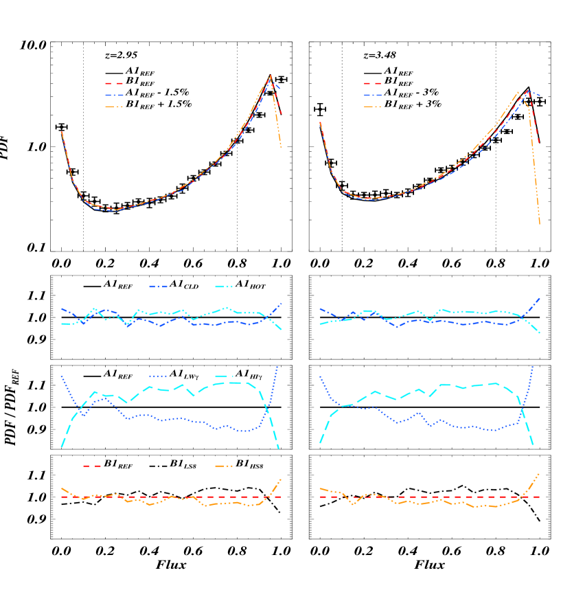
Figure 15: Simulated PDFs at redshift $z=2.95$ (left-hand side) and $z=3.48$ (right-hand side). Upper two panels: Our two reference simulations are displayed in both plots: run A1_REF (black solid curves) and run B1_REF (red dashed curves). The black data points show the PDF measured from the full observational sample after the removal of metals and LLS (Tab. 2, last two columns). The blue dot-dashed curves and orange triple dot-dashed curves are the PDFs obtained with $\pm 1.5\%$ (left-hand side) and $\pm 3\%$ (right-hand side) continuum errors added to the spectra from the runs A1_REF and B1_REF, respectively. The two vertical dotted lines mark the region inside which we perform the fit to the observational data in this work. Lower six panels: the ratio between PDFs obtained from simulations with different values of astrophysical and cosmological parameters, and the corresponding reference PDF_REF. Variations in the following parameters are explored: $T_{\rm 0}$ (first row), $\gamma$ (second row) and $\sigma_{\rm 8}$ (third row).

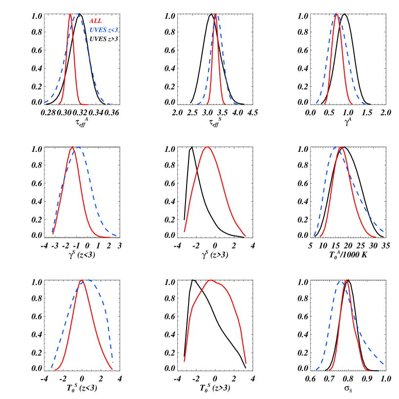
Figure 16: One-dimensional marginalized constraints on the cosmological and astrophysical quantities used in the analysis (see text for details of the parametrization). The blue curves indicate the constraints obtained by using the PDF measurements at $z<3$ presented by K07 (see also the analysis of Viel, Bolton & Haehnelt 2009), black-continuous curves refer to the present work, while the joint constraints for both this data set and the measurements of K07 are shown as continuous red curves.

Table 5: $1-\sigma$ parameter constraints from the sample of QSOs analysed in $a)$ this work and $b)$ the joint sample composed of this work and the K07 PDF data.

		$\tau_{\rm eff}^{\rm A}$	$\tau_{\rm eff}^{\rm S}$	$\gamma^{\rm A}$	$\gamma^{\rm S}(z<3)$	$\gamma^{\rm S}(z>3)$	$T_{\rm 0}^{\rm A}$ [K]	$T_{\rm 0}^{\rm S}$ ($z<3$)	$T_{\rm 0}^{\rm S}$ ($z>3$)	$\sigma_{\rm 8}$
	this work	0.322	3.15	0.90	–	-1.8	19250	–	-0.8	0.8
		$\pm$0.012	$\pm$0.28	$\pm$0.21		$\pm$1.0	$\pm$4800		$\pm$1.5	$\pm$0.04
	this work + K07 data	0.308	3.26	0.70	-1.4	-0.6	17900	0.1	-0.1	–
		$\pm$0.005	$\pm$0.10	$\pm$0.12	$\pm$0.7	$\pm$1.3	$\pm$3500	$\pm$1.0	$\pm$1.6

5.2 Constraints on cosmological and astrophysical parameters

We next use the synthetic spectra to construct flux PDFs which may be compared to our observational measurements. We explore the effect of varying the following cosmological and astrophysical parameters on the PDF: $\sigma_{\rm 8}$, $n_{\rm s}$, $\Omega_{\rm 0m}$ and $H_{\rm 0}$ for the cosmological parameters, and $T_{\rm 0}$ and $\gamma$ for the IGM thermal history. Note, however, that most of the cosmological parameters are only weakly constrained by the flux PDF. The largest effect is induced by using a different value of $\sigma_{8}$ (e.g. Bolton et al. 2008). We will therefore present marginalized cosmological constraints for the amplitude of the matter power spectrum only. The astrophysical parameters $T_{\rm 0}$ and $\gamma$ are parameterized as a broken power-law around $z=3$, in order to investigate possible changes in the thermal state around HeII reionization: $T_{0}=T_{0}^{\rm A}(z=3)\times[(1+z)/4]^{T_{0}^{\rm S}(z)}$ and $\gamma=\gamma^{\rm A}(z=3)\times[(1+z)/4]^{\gamma^{S}(z)}$ (Viel et al. 2009). The effective optical depth evolution is parameterized $\tau_{\rm eff}=\tau_{\rm eff}^{\rm A}(z=3)\times[(1+z)/4]^{\tau_{\rm eff}^{\rm S}(z)}$.

In order to explore our parameter space efficiently with our limited number of simulations, we Taylor expand the flux PDF and compute derivatives to second order using two simulations (plus the reference run) for each parameter. This closely follows the procedure described in Viel & Haehnelt (2006), where this Taylor expansion method was used in order to explore constraints derived from the Sloan Digital Sky Survey flux power spectrum (McDonald et al. 2006). We start with the A1_REF simulation and proceed to calculate the $\chi^{2}$ of our models by varying all the parameters that alter the flux PDF, enabling us to expand around the fiducial starting model. The expansion method allows us to explore the parameter space close to the reference model with an accurate set of hydrodynamic simulations, even if the full parameter space cannot be probed in this way with the same high accuracy. We impose weak priors on the effective optical depth evolution, but both its amplitude and slope are constrained strongly by the data, so the priors do not affect our results. In order to present a conservative analysis, we also decide to consider only the values of the flux in the range $F=[0.1-0.8]$, as this range should not be affected much by the errors made in the continuum fitting procedure (e.g. K07; Bolton et al. 2008, and see Fig. 8). Furthermore, when estimating the covariance between the PDF data points we use the covariance extracted from the simulations for the non-diagonal terms, which is less noisy (e.g. Lidz et al. 2006).

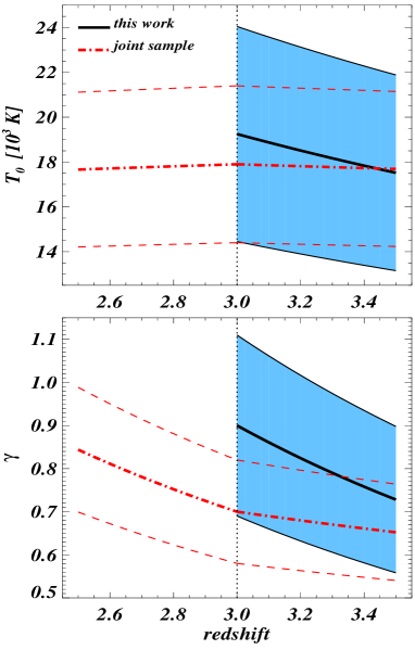
Figure 17: Redshift evolution of the temperature at the mean density, $T_{0}$, (upper panel), and the slope of the temperature-density relation, $\gamma$, (lower panel) inferred from our analysis of the flux PDF. The black solid lines are the results obtained from this work ($z>3$), with the shaded blue regions showing the associated errors (see text for details). The red dot-dashed and lines are the results obtained considering the joint sample composed of this work and the K07 data. The associated errors are shown by the red dashed lines. The vertical black dotted lines mark the transition between $z<3$ and $z>3$.

The one dimensional marginalized constraints are shown in Figure 16: the likelihoods obtained in the present work are represented by the black curves, while the results derived from $z<3$ K07 data set analysed by Viel et al. (2009) are shown as dashed blue lines. The joint constraints for both PDF measurements are plotted as the red lines. From this figure we can see that overall there is agreement between the inferred parameter values for the high redshift (this work) and low redshift (K07) measurements. The $1-\sigma$ parameter constraints from the sample of QSOs analysed in this work and for the joint sample including the K07 data are summarized in Tab. 5. The minimum $\chi^{2}$ for the best fitting model to the PDF measured in this work is 52 for 38 degrees of freedom (d.o.f.) which is likely to happen 7 per cent of the time. In contrast, for the joint sample the minimum $\chi^{2}$ is 94 for 83 d.o.f. with has a 21 per cent probability. The probability is calculated using the full covariance matrix for all the parameters recovered. Note that the ”degrees of freedom” value does not have a precise meaning if the error bars are heavily correlated. However, this happens not to be the case in the flux ranges considered here, $F=[0.1$–$0.8]$, where correlations are weak. We have also checked that there is good agreement between the derived constraints from the present data set when compared to constraints obtained by splitting the sample in two and three redshift bins.

5.3 Implications for the IGM thermal history

Finally, in Figure 17 we display the redshift evolution of the temperature at the mean density, $T_{0}$, and the slope of the temperature-density relation, $\gamma$, inferred from our analysis. We use the broken power-law parameterization around $z=3$ introduced previously: $f=f^{\rm A}\times[(1+z)/4]^{f^{\rm S}(z)}$, where $f=T_{0}$ or $\gamma$, $f^{\rm A}$ is the corresponding normalization factor at $z=3$ and $f^{\rm S}(z)$ is the slope of the relation (see Tab. 5). The black solid lines in Figure 17 are the results obtained from this work ($z>3$) while the shaded blue regions show their associated errors. The red dot-dashed lines are the results obtained from the joint sample composed of this work and the K07 data. The red dashed lines show the associated errors. Since the $f^{\rm A}$ and $f^{\rm S}(z)$ parameters are correlated and the $f^{\rm S}(z)$ are in general poorly constrained, we define the error associated to $f$, at a given redshift $z$, as follows:

$$\Delta f=\left(f^{\rm A}_{\rm ul}-f^{\rm A}_{\rm ll}\right)\times\left(\frac{1+z}{3}\right)^{f^{\rm S}(z)},$$ (7)

where $f^{\rm A}_{\rm ul}=f^{\rm A}+1\sigma$ and $f^{\rm A}_{\rm ll}=f^{\rm A}-1\sigma$ are, respectively, the $1-\sigma$ upper and lower limits on $f^{\rm A}$, and ${f^{\rm S}(z)}$ are the best fit values of the slope showed in Tab. 5.

The temperature at mean density and its redshift evolution, shown in the upper panel of Figure 17, are not strongly constrained by the flux PDF, although our measurements are consistent with other recent analyses presented in the literature which hint that HeII reionization may be completing around $z\simeq 3$ (Lidz et al. 2010, Becker et al. 2011). However, the PDF constraints alone are not precise enough to draw conclusions about the timing and extent of HeII reionization; the flux PDF is a relatively insensitive to $T_{0}$ (see e.g Fig. 15). Alternative measurements from Doppler widths (Schaye et al 2000) wavelets (Lidz et al. 2010) or the curvature statistic (Becker et al. 2011) are typically better suited for this measurement.

On the other hand, the flux PDF is sensitive to the slope of the temperature-density relation, $\gamma$. The constraints displayed in Fig. 17, based on the PDF measurements presented in this work, are formally consistent with an isothermal temperature-density relation at $z=3$ (i.e. $\gamma\sim 1$), although the uncertainties remain large. A temperature-density relation which is close to isothermal may be expected if HeII reionization was underway by $z=3$ (e.g. Schaye et al. 2000, Theuns et al. 2002). When combining our data with the K07 measurements at lower redshift, however, the inferred $\gamma$ at $z=3$ is shifted to lower, inverted $(\gamma<1)$ values, consistent with previous results based on the K07 data (e.g. Bolton et al. 2008, Viel et al. 2009). This is because the K07 data is more constraining at $z\leq 3$ due to the larger number of QSOs in this sample, and for the simple power-law parameterisation we have assumed this also pushes our joint constraints to smaller $\gamma$ values at $z\geq 3$.

It has been suggested recently that an inverted temperature-density relation at may be explained by an IGM which is volumetrically heated by TeV emission from blazars (e.g. Chang et al. 2011, Puchwein et al 2011). This is in contrast to conventional photo-ionization heating models which predict a temperature-density relation which evolves from isothermal to $\gamma\sim 1.6$ following reionization (Hui & Gnedin 1997). We caution, however, the uncertainties on the flux PDF measurements are still large; the temperature-density relation suggested by the radiative transfer simulations of McQuinn et al. (2011), $\gamma\sim 1.3$ at $z=3$, is compatible at the $1.5\sigma$ level with the value derived from the sample considered in this work alone. The K07 data alone are furthermore consistent with an isothermal IGM, again to within $1.5\sigma$ (Viel et al. 2009). We conclude that tighter constraints on $\gamma$ from larger data sets, as well as a comparison of different measurement techniques to aid with the identification possible systematics, will be required for distinguishing between different IGM heating scenarios.

6 Conclusions

In this paper, we have measured the Lyman $\alpha$ forest flux PDF from a set of eight QSO spectra to investigate the thermal state of the IGM at $z\simeq 3$. The absorption lines in the Lyman $\alpha$ forest have been fitted with Voigt profiles, and absorption lines arising from heavy elements have been carefully identified. The spectra have then subsequently had the metal absorption lines removed from within the Lyman $\alpha$ forest. The resulting masked spectra have been used to study the redshift evolution of the Lyman $\alpha$ forest flux distribution and the evolution of the HI effective optical depth. Our results can be summarized as follows.

• By removing metals from the Lyman $\alpha$ forest, we attempt to eliminate pixels which will introduce a systematic uncertainty into our measurement of the flux PDF. The effect of removing these metals on the PDF is to decrease the number of pixels in bins of low flux and increase the number of pixels in bins of high flux. As a result, the PDF measured after correcting for metal absorption is slightly steeper than the PDF measured without removing metals. In general, the effect of metal removal on the PDF is strongest for flux bins at $F<0.6$, in agreement with previous results for other QSO samples at lower redshift (K07).
  

• We measure the PDF for our full sample in two redshift bins, both before and after metal decontamination, and find the effect of metal absorption on the Lyman $\alpha$ forest flux PDF is redshift dependent. It is more significant at lower redshift, where the average opacity of the Lyman $\alpha$ forest is lower and there are fewer absorption lines. This redshift dependence may be understood in terms of the larger number of metal lines which are blended with Lyman $\alpha$ absorption lines toward higher redshift, resulting in the identification of fewer isolated metal absorption lines. On the other hand, it is also possible that the metallicity of the intergalactic medium decreases with increasing lookback time.
  

• We present measurements of the effective optical depth, $\tau_{\rm eff}$, from our QSO sample, which provides a probe of the IGM which is complementary to the PDF. The values of $\tau_{\rm eff}$ measured from the QSOs in our sample can be fitted with a power-law $\tau_{\rm eff}=0.0028\pm 0.0003\,(1+z)^{3.45\pm 0.08}$, in agreement with previous measurements by K07 after correcting for metal absorption. We also find no substantial evidence for a deviation from a power law in the $\log(\tau_{\rm eff})-\log(1+z)$ plane at $z\simeq 3.2$.
  There is a weak redshift dependence of the ratio of the HI effective optical depth measured before and after removing identified metal absorption lines. The ratio increases toward lower redshift, and is consistent with our previous finding from the PDF that metal absorption plays a more significant role in the Lyman $\alpha$ forest toward lower redshift.
  

• We perform a set of high resolution hydrodynamical simulations with a range of cosmological and astrophysical parameters and use them to extract mock QSO spectra with properties that closely resemble those of the observed spectra. We compute the Lyman $\alpha$ flux PDF and compare it to the observed PDF in the range $F=[0.1$–$0.8]$ via a Taylor expansion at second order to find deviations from a best-guess case (e.g. Viel & Haehnelt 2006). By implementing this method within a Monte Carlo Markov Chain likelihood estimator, we present constraints for the IGM thermal state. At $z=3$, our PDF measurements are consistent with an isothermal temperature-density relation, $\gamma=0.90\pm 0.21$, and a temperature at the mean density of $T_{0}=19250\pm 4800$ K (1$\sigma$ uncertainties).
  

• We also obtain joint constraints on the IGM thermal state by analysing the lower redshift PDF measurements of K07, which is a significantly larger data set than the one considered here. At $z=3$, we find the joint data set is consistent with an inverted temperature-density relation, $\gamma=0.70\pm 0.12$, with $T_{0}=17900\pm 3500$ K (1$\sigma$ uncertainties).
  

• In conclusion, the present work highlights the role of the flux PDF as a competitive and quantitative thermometer which may be used to constraint the IGM temperature-density relation over a wide redshift range. The constraints derived from the present work are complementary with respect to other approaches, such as the wavelets method (Lidz et al. 2010), the cutoff in the Doppler width-column density plane (Schaye et al. 2000) or the curvature (Becker et al. 2011), which are primarily sensitive to higher density regions of the IGM at $z\simeq 3$. In the near future, the most promising route to making further progress on our knowledge of the thermal state of the IGM will be to carefully compare and contrast results from these different probes of the IGM temperature-density relation.

References

- [\citeauthoryearBecker et al.2011] Becker G. D., Bolton J. S., Haehnelt M. G., Sargent W. L. W., 2011, MNRAS, 410, 1096
- [\citeauthoryearBergeron et al.2004] Bergeron J., et al., 2004, Msngr, 118, 40
- [\citeauthoryearBernardi et al.2003] Bernardi M., et al., 2003, AJ, 125, 32
- [\citeauthoryearBolton et al.2008] Bolton J. S., Viel M., Kim T.-S., Haehnelt M. G., Carswell R. F., 2008, MNRAS, 386, 1131
- [\citeauthoryearBolton et al.2009] Bolton J. S., Oh S. P. and Furlanetto S. R, 2009a, MNRAS, 395, 736
- [\citeauthoryearBolton et al.2009] Bolton J. S., Oh S. P. and Furlanetto S. R, 2009b, MNRAS, 396, 2405
- [Chang et al.(2011)Chang, Broderick, & Pfrommer] Chang, P., Broderick, A. E., & Pfrommer, C. 2011, ApJ submitted, (arXiv:1106.5504)
- [Croft et al.(2002)Croft, Weinberg, Bolte, Burles, Hernquist, Katz, Kirkman, & Tytler] Croft, R. A. C., Weinberg, D. H., Bolte, M., Burles, S., Hernquist, L., Katz, N., Kirkman, D., & Tytler, D. 2002, ApJ, 581, 20
- [\citeauthoryearDall’Aglio et al.2008a] Dall’Aglio A., Wisotzki L., Worseck G., 2008a, A&A, 480, 359
- [\citeauthoryearDall’Aglio et al.2008b] Dall’Aglio A., Wisotzki L., Worseck G., 2008b, A&A, 491, 465
- [\citeauthoryearDesjacques et al.2007] Desjacques, V., Nusser, A., Sheth, R. K., 2007, MNRAS, 374, 206
- [\citeauthoryearD’Odorico et al.2010] D’Odorico V., Calura F., Cristiani S., Viel M., 2010, MNRAS, 401, 2715
- [\citeauthoryearDekker et al.2000] Dekker H., D’Odorico S., Kaufer A., Delabre B., Kotzlowski H., 2000, SPIE, 4008, 534
- [\citeauthoryearEisenstein & Hu1999] Eisenstein D. J., Hu W., 1999, ApJ, 511, 5
- [Faucher-Giguère et al.(2008)Faucher-Giguère, Prochaska, Lidz, Hernquist, & Zaldarriaga] Faucher-Giguère, C.-A., Prochaska, J. X., Lidz, A., Hernquist, L., & Zaldarriaga, M. 2008, ApJ, 681, 831
- [\citeauthoryearHaardt & Madau2001] Haardt F., Madau P., 2001, cghr.conf, XXXVIth Rencontres de Moriond , XXIst Moriond Astrophysics Meeting, March 10-17, 2001 Savoie, France. Edited by D.M. Neumann & J.T.T. Van. http://moriond.in2p3.fr
- [\citeauthoryearHeap et al.2000] Heap S. R., Williger G. M., Smette A., Hubeny I., Sahu M. S., Jenkins E. B., Tripp T. M., Winkler J. N., 2000, ApJ, 534, 69
- [\citeauthoryearHui & Gnedin1997] Hui L., Gnedin N. Y., 1997, MNRAS, 292, 27
- [\citeauthoryearJarosik et al.2011] Jarosik N., et al., 2011, ApJS, 192, 14
- [\citeauthoryearKim et al.2007] Kim T.-S., Bolton J. S., Viel M., Haehnelt M. G., Carswell R. F., 2007, MNRAS, 382, 1657 (K07)
- [\citeauthoryearKim, Cristiani, & D’Odorico2002] Kim T.-S., Cristiani S., D’Odorico S., 2002, A&A, 383, 747
- [\citeauthoryearKomatsu et al.2009] Komatsu E., et al., 2009, ApJS, 180, 330
- [\citeauthoryearKriss et al.2001] Kriss G. A., et al., 2001, Sci, 293, 1112
- [\citeauthoryearLidz et al.2006] Lidz A., Heitmann K., Hui L., Habib S., Rauch M., Sargent W. L. W., 2006, ApJ, 638,
- [Lidz et al.(2010)Lidz, Faucher-Giguère, Dall’Aglio, McQuinn, Fechner, Zaldarriaga, Hernquist, & Dutta] Lidz, A., Faucher-Giguère, C.-A., Dall’Aglio, A., McQuinn, M., Fechner, C., Zaldarriaga, M., Hernquist, L., & Dutta, S. 2010, ApJ, 718, 19927
- [\citeauthoryearLee2012] Lee K.-G., 2012, ApJ, submitted, (arXiv:1103.2780)
- [\citeauthoryearLee2012] Lee, K.-G.; Suzuki, N.; Spergel, D. N., 2012, AJ, 143, 51
- [\citeauthoryearMcDonald et al.2000] McDonald P., Miralda-Escudé J., Rauch M., Sargent W. L. W., Barlow T. A., Cen R., Ostriker J. P., 2000, ApJ, 543, 1
- [\citeauthoryearMcDonald et al.2001] McDonald P., Miralda-Escudé J., Rauch M., Sargent W. L. W., Barlow T. A., Cen R., 2001, ApJ, 562, 52
- [\citeauthoryearMcDonald et al.2006] McDonald P., et al., 2006, ApJS, 163, 80
- [McQuinn et al.(2009)McQuinn, Lidz, Zaldarriaga, Hernquist, Hopkins, Dutta, & Faucher-Giguère] McQuinn, M., Lidz, A., Zaldarriaga, M., Hernquist, L., Hopkins, P. F., Dutta, S., & Faucher-Giguère, C.-A. 2009, ApJ, 694, 842
- [\citeauthoryearMcQuinn et al.2011] McQuinn M., Hernquist L., Lidz A., Zaldarriaga M., 2011, MNRAS, 415, 977
- [Pâris et al.(2011)] Pâris, I., Petitjean, P., Rollinde, E., et al. 2011, A&A, 530, A50
- [\citeauthoryearPuchwein et al.2011] Puchwein E., Pfrommer C., Springel V., Broderick A. E., 2011, MNRAS submitted, (arXiv:1107.3837)
- [\citeauthoryearRauch1998] Rauch M., 1998, ARA&A, 36, 267
- [\citeauthoryearReichardt et al.2009] Reichardt C. L., et al., 2009, ApJ, 694, 1200
- [\citeauthoryearReimers et al.1997] Reimers D., Kohler S., Wisotzki L., Groote D., Rodriguez-Pascual P., Wamsteker W., 1997, A&A, 327, 890
- [\citeauthoryearSchaye et al.2000] Schaye J., Theuns T., Rauch M., Efstathiou G., Sargent W. L. W., 2000, MNRAS, 318, 817
- [\citeauthoryearSchaye et al.2003] Schaye J., Aguirre A., Kim T.-S., Theuns T., Rauch M., Sargent W. L. W., 2003, ApJ, 596, 768
- [Shull et al.(2010)Shull, France, Danforth, Smith, & Tumlinson] Shull, J. M., France, K., Danforth, C. W., Smith, B., & Tumlinson, J. 2010, ApJ, 722, 1312
- [\citeauthoryearSongaila1998] Songaila A., 1998, AJ, 115, 2184
- [\citeauthoryearSongaila & Cowie1996] Songaila A., Cowie L. L., 1996, AJ, 112, 335
- [\citeauthoryearSpringel2005] Springel V., 2005, MNRAS, 364, 1105
- [Syphers et al.(2011)Syphers, Anderson, Zheng, Meiksin, Haggard, Schneider, & York] Syphers, D., Anderson, S. F., Zheng, W., Meiksin, A., Haggard, D., Schneider, D. P., & York, D. G. 2011, ApJ, 726, 111
- [\citeauthoryearTescari et al.2011] Tescari E., Viel M., D’Odorico V., Cristiani S., Calura F., Borgani S., Tornatore L., 2011, MNRAS, 411, 826
- [\citeauthoryearTheuns et al.1998] Theuns T., Leonard A., Efstathiou G., Pearce F. R., Thomas P. A., 1998, MNRAS, 301, 478
- [\citeauthoryearTheuns et al.2002] Theuns T., Bernardi M., Frieman J., Hewett P., Schaye J., Sheth R. K., Subbarao M., 2002, ApJ, 574, L111
- [\citeauthoryearViel & Haehnelt2006] Viel M., Haehnelt M. G., 2006, MNRAS, 365, 231
- [\citeauthoryearViel, Bolton, & Haehnelt2009] Viel M., Bolton J. S., Haehnelt M. G., 2009, MNRAS, 399, L39
- [Viel et al.(2004)Viel, Haehnelt, & Springel] Viel, M., Haehnelt, M. G., & Springel, V. 2004, MNRAS, 354, 684
- [Worseck et al.(2011)Worseck, Prochaska, McQuinn, Dall’Aglio, Fechner, Hennawi, Reimers, Richter, & Wisotzki] Worseck, G. et al. 2011, ApJL, 733, L24
- [\citeauthoryearZaldarriaga, Hui, & Tegmark2001] Zaldarriaga M., Hui L., Tegmark M., 2001, ApJ, 557, 519