Optimal obstacle placement with disambiguations

Abstract

We introduce the optimal obstacle placement with disambiguations problem wherein the goal is to place true obstacles in an environment cluttered with false obstacles so as to maximize the total traversal length of a navigating agent (NAVA). Prior to the traversal, the NAVA is given location information and probabilistic estimates of each disk-shaped hindrance (hereinafter referred to as disk) being a true obstacle. The NAVA can disambiguate a disk’s status only when situated on its boundary. There exists an obstacle placing agent (OPA) that locates obstacles prior to the NAVA’s traversal. The goal of the OPA is to place true obstacles in between the clutter in such a way that the NAVA’s traversal length is maximized in a game-theoretic sense. We assume the OPA knows the clutter spatial distribution type, but not the exact locations of clutter disks. We analyze the traversal length using repeated measures analysis of variance for various obstacle number, obstacle placing scheme and clutter spatial distribution type combinations in order to identify the optimal combination. Our results indicate that as the clutter becomes more regular (clustered), the NAVA’s traversal length gets longer (shorter). On the other hand, the traversal length tends to follow a concave-down trend as the number of obstacles increases. We also provide a case study on a real-world maritime minefield data set.

and

1 Introduction

A challenging stochastic optimization problem that has practical applications in robotics, computer vision and naval logistics is the stochastic obstacle scene (SOS) problem. This problem was first introduced by Papadimitriou and Yannakakis (1991), and its graph-theoretic version was called the Canadian traveler’s problem. Both continuous and graph-theoretic versions of the problem have gained considerable attention recently [see, e.g., Nikolova and Karger (2008), Xu et al. (2009), Likhachev and Stentz (2009), Eyerich, Keller and Helmert (2009), Aksakalli et al. (2011)]. In this article, we consider a slightly modified version of the original SOS problem. In this version, a point-sized navigating agent (NAVA) needs to quickly traverse from a given starting point to a target point through an arrangement of disk-shaped regions (these regions shall be referred to as “disks” henceforth for brevity). Some of these disks are true obstacles placed by another agent, called the obstacle-placing agent (OPA), and the rest is clutter, that is, false obstacles. For instance, in case of a naval logistics application, the true obstacles would be mines, and the clutter could be rocks, metal pieces, debris, etc. The OPA places the true obstacles in between the clutter prior to the NAVA’s traversal. At the outset, the NAVA does not know the actual status of any disk. However, the NAVA is given respective probabilities of each disk being a true obstacle or a clutter. Over the course of the traversal, the NAVA has the option to disambiguate any (ambiguous) disk, that is, learn with 100% accuracy if it is a true obstacle. This disambiguation can be performed when the NAVA is situated on a disk’s boundary. The NAVA can pass through a disk only if a disambiguation reveals that it is clutter, that is, not a true obstacle. We assume that there is no limit on the number of available disambiguations, and that disambiguations can be executed only at a cost added to the overall length of the traversal. We also assume that the obstacle scene is static, that is, the disks do not change location during the traversal, and the obstacle/clutter status of a disk never changes. The NAVA’s challenge is to decide what and where to disambiguate en route so as to minimize the total length of the traversal. This problem is called the SOS problem. The OPA’s challenge, on the other hand, is to place a given number of true obstacles in between the clutter so as to maximize the traversal length of the NAVA in a game-theoretic sense. We call this problem the obstacle placement with disambiguations problem, or the OPD problem in short.

As discussed in Aksakalli (2007), the SOS problem can be cast as a Markov decision process, though with exponentially many states. There are no efficiently computable optimal policies known for the SOS problem, and many similar problems have been shown to be intractable [Papadimitriou and Yannakakis (1991), Provan (2003)]. Nonetheless, several efficient heuristics have been proposed for the problem; see, for example, Fishkind et al. (2007) and Aksakalli et al. (2011). In particular, the reset disambiguation (RD) algorithm of Aksakalli et al. (2011) is an efficient heuristic for the SOS problem in a continuous setting. This algorithm is provably optimal for a restricted class of SOS problems, and it has been shown to perform well for general instances of the problem.

Algorithms in the literature for the SOS problem and its variants—both in continuous and discrete settings—have assumed that the spatial distribution of possible-obstacles is given. In general, performance of these algorithms has been evaluated under complete spatial randomness assumption for both true obstacles and clutter. In a broader scheme, there has been some research on detecting (true) obstacles via the obstacle field’s spectral image properties [Priebe, Olson and Healy (1997), Olson, Pang and Priebe (2003)] as well as the field’s spatial point pattern characteristics [Cressie and Lawson (2000), Cressie and Brant Collins (2001), Muise and Smith (1995), Walsh and Raftery (2002)]. These studies, on the other hand, assume that the obstacle field’s spatial point distribution is given. To our knowledge, the important problem of placing the obstacles to maximize a NAVA’s total traversal length, that is, the OPD problem, has not been studied before.

The goal of this article is to introduce the OPD problem and study the problem in one particular setting to stimulate further research on this subject and lay ground for more comprehensive prospective studies. In particular, this study is limited to an investigation of relative efficiency of a variety of obstacle placement schemes against different background clutter types sampled from various spatial point distributions. Our goal is to gain insight into which obstacle placement scheme works better for which clutter type, and explore the effect of the number of obstacles on the NAVA’s traversal length. In particular, we would like to address the following two critical research questions:

• Given a clutter type, what is the optimal number of obstacles and the obstacle pattern to use so as to maximize the NAVA’s total traversal length?

• Obstacles are likely to be costly, and the OPA might not have enough numbers of obstacles. In this case, what is the optimal way to place a given number of obstacles for a given clutter type?

The primary analysis tool we use is repeated measures analysis of variance (ANOVA). Our specific setup leads to a three-way repeated measures ANOVA problem where the treatment factors are as follows:

Clutter type: We consider 6 different point processes for sampling clutter disk centers: homogeneous and inhomogeneous Poisson processes, Matérn and Thomas clustered point processes, and hardcore and Strauss regular point processes.

Number of obstacles: We consider 5 different numbers of obstacles (20, 30, 40, 50, and 60, resp.).

Obstacle layout scheme: We experiment with a total of 19 different obstacle placement patterns. These patterns are sampled from a homogeneous Poisson process within four different window forms: the clutter sampling window itself, linear, V-, and W-shaped polygonal windows.

The response variable here is the total traversal length of the NAVA including the cost of disambiguations. Without loss of generality, we assume a fixed radius for both obstacle and clutter disks. For computational efficiency, we work with an 8-adjacency integer lattice discretization of the continuous setting as in Aksakalli et al. (2011). As for the NAVA’s navigation algorithm, we use a simple adaptation of the RD algorithm for the lattice discretization, which we call the adapted RD (ARD) algorithm.

The rest of this manuscript is organized as follows: The SOS problem is formally defined in Section 2 and the ARD algorithm is outlined in Section 3. The clutter spatial point distributions (i.e., clutter types) are described in Section 4, and the obstacle placement patterns are introduced in Section 5. The experimental setup and the statistical analysis of our Monte Carlo simulations are provided in Section 6. In Section 7 we illustrate our approach on a real-world U.S. Navy minefield data set. Summary, conclusions, and directions for prospective research are presented in Section 8.

2 The SOS and OPD problems

The continuous SOS problem is formally defined as follows: Consider a bounded obstacle field $\Omega\subset\mathbb{R}^{2}$. There exists a clutter spatial point process $\mathcal{C}$ that generates points $X_{C}\subset\Omega$ at which clutter disks are centered. Next, an obstacle-placing agent (OPA) samples disk centers $X_{O}\subset\Omega$ from an obstacle spatial point process $\mathcal{O}$ and places obstacle disks centered at $X_{O}$. A navigating agent (NAVA) wishing to traverse from a given starting point $s\in\Omega$ and a target point $t\in\Omega$ is equipped with a sensor that assigns random marks $\rho_{C}\dvtx X_{C}\rightarrow(0,1]$ and $\rho_{O}\dvtx X_{O}\rightarrow(0,1]$ prior to the NAVA’s traversal. When observing a realization of these processes, the NAVA only sees $X:=X_{C}\cup X_{O}$. We assume that, for all $x\in X$, $\rho(x)$ is the probability that $x\in X_{O}$, that is, $x$ is a true obstacle. For every disk center $x$, the possibly-obstacle disk $D_{x}$ is an open region with a fixed radius $r>0$. The NAVA seeks to traverse a continuous $s,t$ curve in $(\bigcup_{x\in X_{O}}D_{x})^{c}$ of shortest achievable arc length, where $A^{c}$ stands for complement of $A$. We further suppose that there is a dynamic learning capability; specifically, for all $x\in X$, when the curve is on the boundary $\partial D_{x}$, the agent has the option to disambiguate $x$, that is, to learn $x\in X_{O}$ or not, but at a cost $c>0$ added to the length of the curve. The NAVA can pass through disks that have been disambiguated and found to be clutter, but needs to avoid ambiguous disks as well as disks that have been disambiguated and found to be a true obstacle. How the NAVA should route the continuous $s,t$ traversal curve—and where and when the disambiguations should be performed—to minimize the length of this curve is called the continuous SOS problem.

The problem of placing the obstacles so as to maximize the NAVA’s traversal length in the SOS problem is called the OPD problem. In this study, we consider a particular variant of the OPD problem where the OPA knows the clutter spatial point distribution (called clutter type for brevity), but not the exact locations of the clutter disks. The motivation for this variant is that the clutter location information requires specific knowledge of the NAVA’s sensor technology, which is not necessarily accessible to the OPA. Nonetheless, it is still likely that the OPA has information on the spatial distribution of the clutter disks. For instance, rock or debris distribution along a specific coastline might follow a certain spatial point distribution that is known to the OPA. We leave it to future research to study a second variant where the OPA knows the exact locations of the clutter disks.

For computational efficiency, we consider a discrete approximation of the continuous setting on a subgraph of the 8-adjacency integer lattice as in Aksakalli et al. (2011). Specifically, this discretization is the graph $\mathsf{G}$ whose vertices are all of the pairs of integers $i,j$ such that $1\leq i\leq i_{\mathrm{max}}$ and $1\leq j\leq j_{\mathrm{max}}$, where $i_{\mathrm{max}}$ and $j_{\mathrm{max}}$ are given integers. There are edges between all pairs of the following four types of vertices: (1) $(i,j)$ and $(i+1,j)$ with unit length, (2) $(i,j)$ and $(i,j+1)$ with unit length, (3) $(i,j)$ and $(i+1,j+1)$ with length $\sqrt{2}$, and (4) $(i+1,j)$ and $(i,j+1)$ with length $\sqrt{2}$. One vertex in $\mathsf{G}$ is designated as the starting point $s$, another vertex in $\mathsf{G}$ is designated as the target point $t$. The NAVA is to traverse from $s$ to $t$ in $\mathsf{G}$, only using edges that do not intersect any true obstacles or ambiguous disks. If an edge intersects any ambiguous disk, then a disambiguation of the obstacle may be performed from either of the edge’s endpoints that is outside of the disk. As before, the goal is to devise an algorithm that minimizes the expected length of the traversal by effective exploitation of the disambiguation capability. We call this discretization the discretized SOS problem, which, in effect, is a special case of the Canadian Traveler’s Problem in the literature with statistical dependency among the edges. The reader is referred to Fishkind et al. (2007) for a review of the literature that includes the history and development of the problems that fall under the SOS problem umbrella.

3 Adaptation of the reset disambiguation algorithm for the discretized SOS problem

The reset disambiguation (RD) algorithm introduced in Aksakalli et al. (2011) for the continuous SOS problem is a high performing heuristic that is provably optimal for a related problem and also optimal for a restricted class of instances for the original SOS problem. Otherwise, the algorithm is generally suboptimal, but it is both effective and efficiently computable. This algorithm can be adapted to the discretized SOS problem as follows: We first define the edge weight function below for each edge in $\mathsf{G}$:

$$w(e):=\ell(e)+\frac{1}{2}\sum_{i=1}^{|X|}\mathbf{1}_{e\cap D_{i}\neq\varnothing}\biggl{(}\frac{c}{1-\rho_{i}}\biggr{)},$$ (1)

where $\ell(e)$ is the Euclidean length of the edge (which is either 1 or $\sqrt{2}$), and $\mathbf{1}$ is the indicator function (taking value 1 or 0 depending on whether its subscripted expression is true or false). For instance, weight of an edge not intersecting any disks is equal to its Euclidean length. On the other hand, weight of an edge intersecting a single disk is equal to the sum of the edge’s Euclidean length and the cost of disambiguation divided by the probability that the disk is not an obstacle. The adapted RD (ARD) algorithm would then have the NAVA do the following:

[(1)]

Find the shortest $s,t$ walk in $\mathsf{G}$ with respect to the edge weights specified by (1) (using, e.g., Dijkstra’s algorithm). Start from $s$ and traverse this walk until its first ambiguous edge $e$ is encountered at vertex $v$, with edge $e$ intersecting disk $D_{i}$. Notice that the NAVA might revisit a vertex over the course of the traversal, making the NAVA’s final trajectory a walk (and not a path).

At this point (since the NAVA cannot enter an ambiguous disk) disambiguate the disk $D_{i}$.

Either remove disk $D_{i}$’s center point $X_{i}$ from $X$ or set $\rho_{i}:=1$ depending on whether $D_{i}$ was just discovered to be, respectively, a clutter or an obstacle.

Repeat this procedure using $v$ as the new $s$ until $t$ is reached.

Figure 1 illustrates the SOS and OPD problem settings with three disks. Two of these disks are clutter and the third one is a true obstacle placed by the OPA. Clutter disks are centered on the sides at $(6,9)$ and $(17,9)$, and the obstacle disk is centered in the middle at $(11,6)$. The clutter disks will be referred to as $D_{1}$ and $D_{2}$, respectively, and the obstacle disk will be referred to as $D_{3}$. It is important to reiterate that in the variant we consider, the OPA knows the clutter distribution type, but not the exact locations of clutter disks. In this specific example, the OPA does not know where $D_{1}$ and $D_{2}$ are located, but simply chooses to place $D_{3}$ at $(11,6)$. Each disk has a radius of 4.5 units and the cost of disambiguation is taken as 5 units. Actual status of the obstacle field is shown in Figure 1(a) where clutter disks are shown as dashed circles and the true obstacle is shown as a solid circle. The NAVA knows locations of all the disks a priori, but does not know which disks are clutter and which ones are truly obstacles. Instead, the NAVA is equipped with sensor technology that assigns respective probabilities to each disk being a true obstacle. These marks for $D_{1},D_{2}$ and $D_{3}$ are taken as 0.4, 0.5 and 0.6, respectively. Shown in Figure 1(b) is how the NAVA sees the obstacle field where gray scale of disks reflects the probability of each disk being a true obstacle as measured via the NAVA’s sensors prior to the NAVA’s traversal, with darker colors indicating higher probabilities of being a true obstacle. Figure 1(c) shows our lattice discretization and the NAVA’s actual traversal. Here, the lattice used is $22\times 14$, with $s=(11,14)$ and $t=(11,1)$. The ARD algorithm first dictates that $D_{3}$ is disambiguated at $(11,11)$. Since this is a true obstacle, $\rho_{1}$ is set to 1 and the algorithm is queried again. This time, the algorithm dictates that $D_{1}$ is disambiguated, again at $(11,11)$. Since $D_{1}$ is clutter, the NAVA passes through it while avoiding $D_{3}$ and reaches the target point. The NAVA’s total traversal length in this case is 29.49 including the cost of the two disambiguations.

(a) The obstacle field	(b) The obstacle field as seen by the NAVA

(c) NAVA’s traversal

Figure 1: A simple setting with three disks and the NAVA’s traversal as dictated by the ARD algorithm. (a) shows the actual status of the obstacle field. The two clutter disks on the sides are denoted by dashed circles and the true obstacle in the middle is denoted by a solid circle. (b) illustrates how the NAVA sees the obstacle field prior to the navigation. Gray scale of disks reflects marks of each disk, with darker colors indicating a higher mark (for being a true obstacle). (c) shows the lattice discretization and the NAVA’s actual traversal.

In our computational experiments, the lattice used is $(i_{\max}\times j_{\max})=(100\times 100)$, with $s=(50,100)$ and $t=(50,1)$. Each disk has a radius of $r=4.5$ units, and the disk centers are sampled on the pairs of real numbers in $[10,90]\times[10,90]$—ensuring that there is always a permissible walk from $s$ to $t$. The cost of disambiguation is taken as $c=5$. As in Priebe et al. (2005), clutter marks are sampled from $\operatorname{Beta}(6,2)$ (with a mean of 0.25) and obstacle marks are sampled from $\operatorname{Beta}(2,6)$ (with a mean of 0.75). This particular setup has been specifically designed to possess similar characteristics to an actual U.S. Navy minefield data set, called the COBRA data, which was presented in Witherspoon et al. (1995) and later used in Fishkind et al. (2007), Ye and Priebe (2010), and Ye, Fishkind and Priebe (2011). In Section 7 we present an extensive case study on the COBRA data itself.

4 Clutter point distributions

Formally, a spatial point process $X$ is a finite random subset of a bounded region $\Omega\subset\mathbb{R}^{2}$. A realization of this point process, on the other hand, is called a spatial point pattern. Classical literature on the subject mainly identifies three spatial point pattern categories based on the nature of inter-point interactions: (1) independent patterns, (2) cluster patterns where points tend to be close to one another, and (3) regular patterns where points tend to avoid each other [Baddeley (2010)]. In this study, we consider two patterns from each one of these three categories in turn, and this section describes those six spatial point processes used to generate background clutter disk centers in the OPD problem. Classical treatments of general spatial point patterns can be found in Cressie (1993) and Rippley (2004). The reader is referred to Møller and Waagepetersen (2007) for a brief overview of spatial point processes, and to Baddeley (2010) for an excellent coverage of the particular point processes considered in this work.

4.1 Homogeneous and inhomogeneous Poisson processes

In the context of spatial point processes, intensity is the average density of points per unit area in the region over which the point process is defined. In general, the null model in a point pattern analysis is the homogeneous Poisson point process in the plane with constant intensity $\lambda$, which is also called complete spatial randomness (CSR). CSR with intensity $\lambda$ will be denoted by $\operatorname{CSR}(\lambda)$. For any finite region $R$, the CSR point process has four properties: (1) the number of points in $R$ is a Poisson random variable, (2) the number of points in any two disjoint regions $R$ and $R^{\prime}$ are independent random variables, (3) the expected number of points in $R$ is $\lambda\cdot\operatorname{area}(R)$, and (4) the points in $R$ are independently and uniformly distributed.

In the OPD problem, a possible scenario is that the density of the clutter increases from the start point toward the target point or vice versa. For instance, the density of rocks and/or debris along a coast line might increase as one traverses toward the coast. To simulate such a scenario, we consider the inhomogeneous Poisson process. This process is a modification of CSR where the intensity is not constant, but varies from location to location. Specifically, the intensity is a function in two-dimensional Euclidean space. Let $\operatorname{IP}(\lambda(h))$ denote the inhomogeneous Poisson process with intensity $\lambda(h)$ where $h\in\mathbb{R}^{2}$. Here, the intensity function $\lambda(h)$ specifies the values of $\lambda$ on the plane. Properties of $\operatorname{IP}(\lambda(h))$ are the same as those of $\operatorname{CSR}(\lambda)$ with the last two properties modified as follows: ($3^{\prime}$) the expected number of points in $R$ is $\int_{R}\lambda(h)\,dh$, and ($4^{\prime}$) points in $R$ are independently and identically distributed with probability density $f(h)=\lambda(h)[\int_{R}\lambda(h)\,dh]^{-1}$.

4.2 Matérn and Thomas clustered point processes

In many real-world contexts, existence of a point at a specific location increases the probability of other points being located in its vicinity, giving rise to a clustered point process. Some examples include human settlements, plants, stars, galaxies and molecules [Daley and Vere-Jones (2002)]. In particular, it might be more realistic to model clutter type in the OPD problem, such as rock formation and debris dispersal along a coastline, as a clustered point process rather than CSR.

A commonly-encountered cluster point process model in the literature is the doubly-stochastic Poisson process, which is also known as the Cox process. This process is a generalization of the Poisson process where the intensity parameter is randomized [Daley and Vere-Jones (2002)]. In this work, we consider two special cases of the Cox process: Matérn and Thomas point processes.

The Matérn point process, denoted $M(\lambda,\mu,r)$, is constructed by first generating a Poisson point process of “parent” points with intensity $\lambda$. Each parent point is then replaced by a random cluster of points where the number of points in each cluster is sampled from a Poisson distribution with parameter $\mu$. These child points are placed independently and uniformly inside a disk with a fixed radius, $r$, centered at the parent point.

Similar to the Matérn point process, the Thomas process, denoted $T(\lambda,\break\mu,\sigma)$, is constructed by first generating a Poisson point process of “parent” points with intensity $\lambda$. A random cluster of points replaces each parent point with the number of points per cluster being sampled from a Poisson distribution with parameter $\mu$. In contrast with the Matérn point process, positions of these child points in the Thomas point process are isotropic Gaussian displacements centered at the cluster parent location with standard deviation $\sigma$.

4.3 Hardcore and Strauss regular point processes

Another potential scenario in the OPD problem is where there is a “regularity” to the clutter disks. That is, the clutter center points tend to be a certain distance away from the other clutter center points. We consider two regular spatial point patterns with pairwise interactions: the hardcore and Strauss point processes. The probability density function of the hardcore process is that of the Poisson process with intensity $\lambda$ conditioned on the event that no two points generated by the process are closer than $d$ units apart, hence denoted at $\operatorname{HC}(\lambda,d)$. The Strauss process, denoted $S(\lambda,d,\gamma)$, on the other hand, generalizes the hardcore process by incorporating a $\gamma\in[0,1]$ parameter that controls the interaction between the points. The process exhibits more regularity for smaller values of $\gamma$, and less regularity for larger $\gamma$. For $\gamma=0$, the Strauss process becomes a hardcore process, and for $\gamma=1$, it reduces to CSR [Baddeley (2010)].

4.4 The Clutter sampling procedure

In our computational experiments, all spatial point processes—both clutter and obstacle—are simulated via the spatstat package in the R programming environment [Baddeley and Turner (2005)]. This particular package assumes that the point processes extend throughout the two-dimensional Euclidean space, but they are observed inside a sampling window $P$. In our case, the sampling window for the clutter center points is taken as $P=[10,90]\times[10,90]$. In sampling of the inhomogeneous Poisson process, points are generated so that clutter density increases from the top of the obstacle field toward the bottom where the target is located. Specifically, the intensity function is taken as $\lambda(x,y)=0.037e^{(10-y)/40}$ on the sampling window $P$, which results in 100 points on the average.

In sampling of the Matérn and Thomas point processes, we work with $M(10,10,10)$ and $T(10,10,5)$, respectively. As for the hardcore and Strauss processes, we sample from $\operatorname{HC}(100,5)$ and $S(100,5,0.5)$. We use the Metropolis–Hastings algorithm while sampling from the hardcore and Strauss processes, which is essentially a Markov chain whose states are spatial point patterns and its limiting distribution is the desired point process. After running the algorithm for a large number of times, which is 100,000 iterations in our experiments, the state of the algorithm is considered to be a realization of the desired point process [Baddeley (2010)].

Parameter values of all the six clutter types are chosen such that the number of points in any sampled point realization would be roughly 100 on the average. For instance, CSR is sampled with number of points being Poisson(100), and the $h(x,y)$ function we use for the inhomogeneous Poisson process results in 100 points on the average. However, the actual number of points in each clutter realization that we use in our experiments is taken to be exactly 100. This is achieved by rejection sampling, that is, by discarding sampled realizations for which number of points is different than 100. The benefit of fixing the number of clutter disks is that variation in traversal lengths resulting from the different number of clutter disks is removed. Thus, the only source of variation in the background clutter in our computational experiments is the spatial distribution of these 100 clutter disks.

It should be noted that using rejection sampling to achieve 100 points for each point pattern that we simulate actually changes the distribution of the process which has produced the point pattern: these points are now from a process conditional on the number of points in the region being 100. In particular, the homogeneous Poisson process, that is, CSR, conditioned on a specific number of points is in fact a uniform distribution of that many points inside the sampling window. However, the crucial observation here is that these conditional processes share the same interaction behavior as the unconditional ones, and this is sufficient for the purpose of our paper. Figure 2 illustrates sample realizations from the clutter point processes within our simulation environment.

(a) CSR	(b) Inhomogeneous Poisson
(c) Matérn	(d) Thomas
(e) Hardcore	(f) Strauss

Figure 2: Sample realizations from the six background clutter spatial point distributions. The specific distribution parameters used are as follows: (a) $\operatorname{CSR}(100)$, (b) $\operatorname{IP}(0.037e^{(10-y)/40})$, (c) $M(10,10,10)$, (d) $T(10,10,5)$, (e) $\operatorname{HC}(100,5)$ and (f) $S(100,5,0.5)$. These parameters are chosen such that the number of points in any sampled point realization would be about 100 on the average. Rejection sampling was then utilized to have exactly 100 points in all the clutter realizations.

5 Obstacle placement schemes

As mentioned earlier, the goal of the OPA is to place a certain number of true obstacles in the obstacle field under the assumption that the OPA knows the spatial point distribution of the background clutter disks, but not their exact locations. On the other hand, the NAVA only has probabilistic information of each disk being a true obstacle. The NAVA, however, can distinguish true obstacles from the clutter only when situated at a disk’s boundary. In this study, we limit our focus to CSR for sampling true obstacle disk centers within a total of 19 different sampling windows. One might also consider inhomogeneous Poisson process for sampling the obstacle disk centers within these sampling windows. In fact, increasing the obstacle intensity along the $s-t$ line might perhaps increase the NAVA’s traversal length in general. However, we limit our focus to CSR for sampling the obstacle disk centers for the following reasons: First, the OPA might not know the exact starting and target points of the NAVA in practice. Second, the area in which the OPA wishes to place obstacles might not be a square region as in our experiments, but perhaps an entire coastline. Thus, it makes more sense from an operational point of view to sample the true obstacle disk centers with uniform intensity inside their respective polygons.

We consider a total of 19 different sampling windows for the obstacle disk centers. The first sampling window is the polygon $P=[10,90]\times[10,90]$, that is, the sampling window for the background clutter. For the remaining windows, we consider 80-unit long and 10-unit wide polygons as described below:

• 8 different linear windows with their top left corner $y$-coordinate being $90,80,\ldots,20$, and

• 5 different V-shaped and W-shaped windows, respectively, with their top left corner $y$-coordinate being $90,80,\ldots,50$. The difference between the top and bottom $y$-coordinates of each one of these 10 polygons is taken as 50 units.

The obstacle sampling window coinciding with the background clutter window itself is code-named as P. Other sampling windows are code-named by the polygon type (“L,” “V” or “W”, resp.) followed by the top left corner coordinate of the polygon. These 4 polygon shapes will be referred to as obstacle forms.

For example, L70 is the polygon whose four corner points are $(10,70)$, $(90,70)$, $(90,60)$ and $(10,60)$ clock-wise starting with the top left corner. The polygon V70’s six corner points are $(10,70)$, $(50,40)$, $(90,70)$, $(90,60)$, $(50,30)$ and $(10,60)$, again clock-wise starting with the top left corner. Similarly, polygon W70’s ten corner points are $(10,70)$, $(30,40)$, $(50,70)$, $(70,40)$, $(90,70)$, $(90,60)$, $(70,30)$, $(50,60)$, $(30,30)$ and $(10,60)$. The polygon W50, for instance, is the same as W70 shifted down 20 units along the $y$-axis. Thus, the 19 obstacle sampling windows we consider are P, L90, L80$,\ldots,$L20, V90, V80$,\ldots,$V50, and W90, W80$,\ldots,$W50. The reason we consider the same polygon shape placed at different $y$-coordinates is that we are not only interested in which polygon shape is more efficient (in terms of increasing the NAVA’s total traversal length), but also which $y$-coordinate (i.e., distance to the target) is more efficient for a given polygon shape. We do not consider placing true obstacles along a straight horizontal line, as detection of such obstacle patterns by the NAVA would be relatively straightforward—see, for example, Muise and Smith (1995) and Walsh and Raftery (2002) for detecting obstacles laid in such linear patterns.

In order to assess the impact of the number of true obstacles in the OPD problem, we consider five different number of obstacles for each one of the 19 obstacle sampling windows: 20, 30, 40, 50 and 60. As mentioned earlier, CSR conditioned on a specific number of points is in fact a uniform distribution with that many points. Therefore, the obstacles we consider are essentially uniformly distributed inside their respective sampling windows. Realizations of obstacle patterns are denoted by the sampling window followed by the number of obstacles. For instance, P:40 and L70:40 refer to the obstacle patterns sampled within the $P$ and L70 windows, respectively, with 40 obstacle center points inside their respective windows. Figure 3 illustrates sample obstacle center point realizations within the L70, V70 and W70 polygons, respectively, with 40 obstacle center points within each polygon against the CSR clutter shown in Figure 2(a).

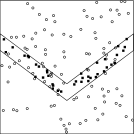
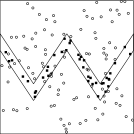
(a) CSR clutter${}+{}$L70:40	(b) CSR clutter${}+{}$V70:40	(c) CSR clutter${}+{}$W70:40

Figure 3: Realizations of obstacle center points inside polygons (indicated by solid boundaries) L70, V70 and W70 with 40 obstacles superimposed on the CSR clutter realization of Figure 1(a). Clutter disk centers are denoted by open circles ($\circ$) and obstacle disk centers are denoted by solid squares ($\blacksquare$).

Shown in Figure 4 is how the NAVA sees the obstacle fields illustrated in Figures 3(b) and 3(c), respectively, and the $s-t$ walks taken by the NAVA as dictated by the ARD algorithm. In Figure 4(a), the NAVA performs a total of 18 disambiguations and the total traversal length (including the cost of disambiguations) is 311.8 units. This particular walk turns out to be rather unfavorable (from the NAVA’s perspective), as the zero-risk $s-t$ walk length avoiding all the disks has a traversal length of merely 151.3 units. Such unfavorable traversals occasionally happen, as the goal of the NAVA is to minimize the expected traversal length, and the actual walk traversed can be much longer than the zero-risk $s-t$ walk based on the outcomes of the disambiguations performed. In Figure 4(b), on the other hand, the NAVA performs only 1 disambiguation and the total traversal length is 152.2 units.

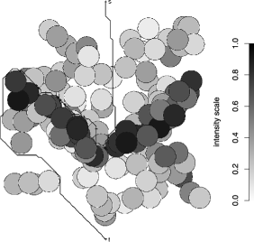
(a) Navigation in CSR clutter${}+{}$V70:40

(b) Navigation in CSR clutter${}+{}$W70:40

Figure 4: The obstacle fields in Figures 3(b) and 3(c) as seen by the NAVA and the NAVA’s navigation in these fields. Gray scale of disks [indicated in (a) as intensity scale] reflects $\rho$ of each disk, with darker colors indicating a higher $\rho$.

6 Experimental setup and the statistical analysis

Our particular experimental setup leads to a three-way ANOVA problem. The treatment factors are the background clutter type, the obstacle placement window and the number of obstacles. The response variable is the NAVA’s total traversal length from $s$ to $t$. The first treatment factor has 6 levels, the second has 19, and the third has 5 levels, resulting in a total of 570 treatment combinations. Our primary goal here is to investigate whether there are any (statistically significant) differences between traversal lengths of different obstacle placement windows for a given number of obstacles and a given clutter type.

For each one of these 570 treatment combinations, we ran 100 Monte Carlo simulations. Each simulation consists of generating the obstacle field (i.e., the obstacle pattern superimposed on a clutter pattern) and executing the ARD algorithm to find the shortest $s-t$ walk. The runtime per simulation averaged over the 57,000 simulations was 9.5 seconds on a personal computer with an Intel Core i7 processor with 2.8 gigahertz clock speed.

As discussed earlier, each background clutter realization is sampled to have exactly 100 clutter disks via rejection sampling. In order to exclude the source of variability due to different clutter realizations for a given clutter type, we adopted a repeated measures approach in our experiments. That is, we sampled only 100 clutter realizations from each one of the 6 clutter types corresponding to each one of the 100 simulations for a given treatment combination. Thus, a total of 600 clutter patterns were generated for our experiments. For instance, the same CSR clutter realization was used for all of the 95 obstacle pattern-obstacle number combinations (19 obstacle patterns and 5 obstacle number levels) for the first Monte Carlo simulation. For the second Monte Carlo simulation, a different CSR realization was sampled and this realization was used for all of the 95 obstacle pattern-obstacle number combinations and so on.

6.1 Repeated measures ANOVA

The background clutter types (abbreviations presented in parentheses) we consider are Complete Spatial Randomness (CSR), inhomogeneous Poisson (IP) distribution, Matérn (M) distribution, Thomas (T) distribution, hardcore (HC) distribution and Strauss (S) distribution. For convenience in presentation, the obstacle types are sometimes numbered from 1 to 19, or labeled in a more descriptive fashion such as V90 which stands for V-shaped obstacle window whose top left corner $y$-coordinate is 90. The 19 obstacle placement window types are sampled within 4 different polygon shapes (a short notation is provided in parentheses): the entire $P$ window (P), linear windows (L), V-shaped windows (V) and W-shaped windows (W). The obstacle window numbering of 1 to 19 corresponds to P, L90, L80$,\ldots,$L20, V90, V80$,\ldots,$V50, W90, W80$,\ldots,$W50, respectively. The obstacle number levels are $20,30,\ldots,60$. As mentioned earlier, for precision in our analysis, we used the same background clutter realization for each of the 95 obstacle types and obstacle number combinations. Thus, we denote the traversal length as $T_{ijkl}$, which is the traversal length of the measurement $l$ for clutter type $i$, obstacle window type $j$, obstacle number level $k$ with $l=1,2,\ldots,100$, $i=1,2,\ldots,6$, $j=1,2,\ldots,19$, and $k=1,2,\ldots,5$, respectively. Clutter types $1,2,\ldots,6$ correspond to CSR, IP, M, T, HC and S patterns, respectively, and obstacle number levels $1,2,\ldots,5$ correspond to $20,30,\ldots,60$, respectively. Note that $T_{ijkl}$, $T_{ij^{\prime}kl}$, $T_{ijk^{\prime}l}$, $T_{ij^{\prime}k^{\prime}l}$ are measured on the same realization of the clutter type $i$, hence, these measures are potentially correlated. In particular, the measurements on consecutive obstacle number levels (with other factors being the same) would be highly (and perhaps positively) correlated. A similar trend can be expected for measurements within each type of obstacle window type (such as linear, V-shaped or W-shaped obstacle forms) as a function of the distance to the target (i.e., as a function of the magnitude of the $y$ coordinate). To take such correlation structure into account, we use repeated measures ANOVA techniques in our analysis to compare the traversal length differences between treatment factors, and possibly existence or lack of any interaction between these factors. Traditionally, repeated measures ANOVA is employed when the measurements are taken on the same subject over time [Kuehl (2000)], but here we are in a similar but nontemporal situation. In our setup, each subject (i.e., background clutter realization) receives all of the 95 treatments (clutter type, obstacle window and obstacle number combinations). Besides, we do not need to randomize the order of the treatments here, since when each treatment combination is applied (i.e., each obstacle pattern is superimposed on the particular clutter realization), we remove the previous data points that come from the other factors. Hence, there is no carry-over effect of the treatments in our study.

The assumptions of repeated measures ANOVA are similar to the standard set of assumptions associated with usual ANOVA, except that independence is not required and an assumption about the relations among the repeated measures (sphericity) is added. The repeated measures ANOVA assumptions are (i) the dependent variable is normally distributed, (ii) homogeneity of covariance matrices, (iii) independence between predictor factors, and (iv) sphericity, which means that the variances of the repeated measures are all equal, and the correlations among the repeated measures are all equal [Tabachnick and Fidell (2006), Howell (2010)].

Repeated measures ANOVA is robust to violations of the first two assumptions [Tabachnick and Fidell (2006)]. Besides, the kernel density plots of the residuals (not presented) resemble that of a Gaussian distribution. (iii) is satisfied by construction in our experimental setup (i.e., the factors clutter type, obstacle type and number of obstacle levels are not dependent). The violation of sphericity is the reason we try various competing variance–covariance structures in addition to compound symmetry (to capture the dependence structure between repeated measures as much as possible). The main benefit of repeated measures ANOVA compared to usual ANOVA is that with repeated measures ANOVA we gain more precision in our results (i.e., the tests are more powerful with more significant $p$-values). Just as using paired differences in the two sample case compared to the two independent samples case increases precision, using repeated measures setup increases the precision compared to usual ANOVA.

In fact, we performed a pilot study to appraise the relative merit of repeated measures ANOVA to usual ANOVA. For the CSR clutter distribution, we generated 5 obstacle number levels (of 20, 30$,\ldots,$60), where obstacle patterns also follow CSR within the sampling window. For the repeated measures ANOVA (called setup I), we used the same CSR clutter realization for each of $20,30,\ldots,60$ obstacles, and we repeated the procedure 100 times (i.e., in total there are 100 different CSR clutter realizations). On the other hand, for the usual ANOVA (called setup II), we used different CSR clutter realizations for each of $20,30,\ldots,60$ obstacles, and we repeated the procedure 100 times (i.e., in total there are 500 different CSR clutter realizations). When the data from setup I was analyzed with repeated measures ANOVA, the obstacle number level was significant (i.e., mean traversal lengths are different for the obstacle number levels) with $F_{4,495}=45.91$, where $F_{4,495}$ stands for $F$ test statistic with degrees of freedom for numerator and denominator being 4 and 495, respectively; on the other hand, when the data from setup II was analyzed with usual ANOVA, the obstacle number level was significant with $F_{4,495}=27.75$. Although the obstacle number is a significant factor in both cases, the repeated measures setup yields a higher level of significance (i.e., more precision and power) compared to the usual ANOVA setup. A similar trend is observed for other clutter and obstacle type levels (not presented), hence, the preference of the current setting over a simple Monte Carlo setup.

In repeated measures ANOVA, we consider (some of or some variants of the) four types of variance–covariance (var–cov) structure: unstructured (UN), autoregressive (AR1), autoregressive heterogeneous (ARH1) and compound symmetry (CS). The CS structure assumes a single variance $\sigma^{2}$ for all treatment combinations and a single covariance $\sigma_{1}$ for each pair of treatment combinations (i.e., sphericity). The CS var–cov structure in our setup with $\sigma_{1}=0$ implies the usual 3-way ANOVA. The UN variance–covariance structure assumes that each variance and covariance is unique, that is, measurements in each of the treatment combinations have a unique variance $\sigma_{i}^{2}$, and each pair of treatment combinations has a unique covariance $\sigma_{ij}$. The AR1 var–cov structure assumes that observations which are close (in some sense) are more correlated than measures that are more distant. For example, the measurements on obstacle numbers 20 and 30 are more correlated than the measurements on obstacle numbers 20 and 60 (with other factors being the same). So there is a single variance $\sigma^{2}$ for all 95 treatment combinations and covariance $\sigma\times\rho^{k}$ where $k$ stands for the order of the measurement. In ARH1 var–cov structure, the variances are also different for the treatment combination levels. So there is a unique variance $\sigma_{i}^{2}$ for each treatment combination, and the covariance structure is as in the autoregressive case [Pinheiro and Bates (2000)]. In our experimental design, it is also possible to further detail the var–cov structure as autoregressive var–cov heterogeneous within only the obstacle factor levels, or heterogeneous within all treatment combinations, or within only the obstacle forms and so on. We also employ Mauchly’s sphericity test to determine the appropriateness of CS var–cov structure in the repeated measures ANOVA [Kuehl (2000)]. That is, we can assume the CS structure only when the Mauchly’s test yields an insignificant $p$-value. In our comparison of the models with various var–cov structures, we apply the model selection criteria as Akaike Information Criteria (AIC) and also perform a $\chi^{2}$ test on the log likelihood function [Burnham and Anderson (2003)].

In what follows, the first section compares overall traversal lengths for the three treatment factors. The next three sections (i.e., Sections 6.2–6.5) present statistical comparison of traversal lengths at clutter type, obstacle form and obstacle number level factors, respectively. The last section gives statistically best performing obstacle type and number combinations at each clutter type.

6.2 Overall comparison of traversal lengths

We first investigate the types and levels of interaction for each pair of treatment combination factors. The profile (or interaction) plots are shown in Figure 5. We also test for interaction between each pair of treatment factors. When obstacle number levels are ignored (i.e., when only interaction between obstacle types/forms and clutter types are considered), we find that obstacle and clutter types do not have significant interaction ($p=0.5258$), neither do obstacle forms and clutter types ($p=0.4811$), which means the trends in mean lengths plotted in Figures 5(a) and (b) are not significantly different from being parallel. Hence, it is reasonable to compare the mean traversal lengths for clutter and obstacle types (i.e., the main effects of clutter and obstacle types), and we find that travel lengths are significantly different between background clutter types ($p<0.0001$) and between obstacle types ($p<0.0001$). Likewise, traversal lengths are significantly different between clutter types ($p<0.0001$) and between obstacle forms ($p<0.0001$). Notice also that, on the average at each obstacle type or form, Matérn and Thomas (i.e., clustered) clutter types tend to yield shorter traversal lengths, while hardcore and Strauss (i.e., regular) clutter types tend to yield longer traversal lengths. Hardcore clutter tends to yield the longest traversal lengths, which suggests that the more regular the clutter type, the longer the traversal lengths. Furthermore, at each obstacle type or form, the average traversal lengths (in ascending order) are for P, W-shaped, linear and V-shaped obstacle forms.

(a)	(b)
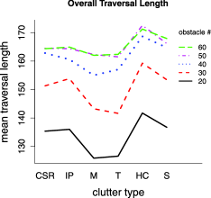
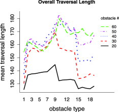
(c)	(d)

(e)

Figure 5: The profile plots for each pair of treatment factors (obstacle type/form, clutter type and obstacle number) when the other factor is ignored.

When clutter types are ignored (i.e., when only interaction between obstacle types/forms and obstacle number levels are considered), we find significant interaction between obstacle type and obstacle number levels ($p<0.0001$), and between obstacle form and obstacle number levels ($p<0.0001$), which means the trends in mean lengths plotted in Figures 5(d) and (e) are significantly nonparallel. Hence, it is not reasonable to compare the mean traversal lengths for obstacle types/forms and obstacle number levels, but instead, for example, it will make sense to compare the mean length values for obstacle number levels at each obstacle type or form. At P and W-shaped obstacle forms, traversal lengths tend to increase as the obstacle number increases; at linear and V-shaped obstacle forms, traversal lengths exhibit a concave-down trend (i.e., increase, reach a peak and then decrease); for the linear and V-shaped windows the shortest lengths occur at 20 obstacles, and longest lengths occur at 40 obstacles. We believe that the concave-down trend is due to the increase in the disk (obstacle and clutter) density that makes the NAVA decide to traverse along the boundary more often, which reduces the traversal length, since the NAVA avoids the disambiguation costs. Hence, a similar concave-down trend (with larger obstacle numbers) is expected to occur for P and W-shaped obstacle forms as well. Moreover, for 20 and 30 obstacles, the highest (average) traversal lengths occur for linear obstacle forms, and for 40–60 obstacles, longest traversal lengths occur for V-shaped obstacle forms. At each obstacle number level, the shortest traversal lengths occur for the P obstacle form.

When obstacle types are ignored (i.e., when only interaction between clutter type and obstacle number levels are considered), we find significant interaction between clutter type and obstacle number levels ($p<0.0001$), which means the trend in mean length plotted in Figure 5(c) is significantly nonparallel. Hence, we compare the mean length values for obstacle number levels at each clutter type. On the average at each clutter type, traversal lengths tend to increase as the obstacle number increases (up to 50 obstacles), but the lengths for 50 and 60 obstacles are very similar. At each obstacle number level, the longest traversal lengths occur for hardcore clutter type, and the shortest traversal lengths occur for Matérn and Thomas clutter types.

The shortest and longest traversal length performances (i.e., the worst and best performances from the OPA perspective) are presented in Table 1. In our overall comparison, the shortest length is about 116 units which occurs at T:W60:20, T:P:20 and M:P:20 treatment combinations, and the longest length is about 190 which occurs at HC:V90:50 treatment combination. Our initial (overall) interaction analysis suggests that it is more reasonable to compare the lengths for each pair of treatment factors at specific levels of the other factor different from both factors in the pair.

In Sections 6.3–6.5, the profile plots, model comparison tables and their detailed discussions are deferred to the technical report Aksakalli and Ceyhan (2012).

Table 1: The shortest and longest traversal lengths and the corresponding treatment types for overall comparisons, and comparisons at specific clutter types, obstacle forms and obstacle numbers

	Shortest		Longest
	Traversal	Treatment	Traversal	Treatment
	length (s)	type (s)	length (s)	type (s)
Overall
	116.16, 116.47,	T:W60:20, T:P:20,	190.29	HC:V90:50
	116.77	M:P:20
Clutter type
CSR	127.56, 127.76	P:20, W60:20	178.68, 178.98,	V70:50, V50:40,
			179.12	V80:50
Inhom.	126.87	W90:20	188.96	V90:60
Poisson
Matérn	116.77	P:20	184.39	V90:50
Thomas	116.16, 116.47	W60:20, P:20	181.48	V90:60
Hardcore	134.42, 134.85,	W80:20, W90:20,	190.29	V90:50
	135.05, 135.50,	W70:20, W50:20,
	135.81, 135.95	P:20, W60:20
Strauss	128.47	P:20	188.35, 188.77	V90:50, V80:40
Obstacle form
CSR	116.47, 116.77	T:20, M:20	163.86	HC:60
Linear	127.32	L40:M:20	184.42	L20:HC:40
V-Shaped	119.23	V50:T:20	190.29	V90:HC:50
W-Shaped	116.16	W60:T:20	176.91, 177.18,	W50:HC:60, W80:HC:60,
			177.36, 177.56,	W50:S:60, W60:T:60,
			177.76	W80:S:60
Number of obstacles
20	116.16, 116.47,	T:W60, T:P,	156.27	HC:L40
	116.77	M:P
30	121.73, 122.25	T:P, M:P	179.43	HC:L20
40	128.95	M:P	187.57, 188.77	HC:V80, S:V80
50	135.04	M:P	190.29	HC:V90
60	143.09	T:P	188.96	IP:V90

6.3 Analysis of traversal lengths at each background clutter type

We investigate and test the interaction between obstacle type/form and obstacle number at each background clutter type. At each background clutter type, we find significant interaction between obstacle form and obstacle number levels ($p<0.0001$ for each) and between obstacle type and obstacle number levels ($p<0.0001$ for each), hence, we do not test for the main effects of obstacle types/forms and obstacle number levels. At each background clutter type, on the average at P and W-shaped obstacle forms, traversal lengths tend to increase as the obstacle number increases; at linear and V-shaped obstacle forms, traversal lengths exhibit a concave-down trend: The longest lengths occur at 40 obstacles for each obstacle form at CSR and Strauss clutter, and for linear obstacles at inhomogeneous Poisson, Thomas and hardcore clutters and at 50 or 60 obstacles for V-shaped obstacles at inhomogeneous Poisson, Thomas and hardcore clutters. The shortest lengths occur at 20 obstacles.

The shortest and longest traversal lengths together with the corresponding treatment combinations are presented in Table 1. Presented below is further discussion on traversal lengths for each clutter type.

CSR clutter: The shortest traversal length is about 127 which occurs at P:20, W60:20 treatment types, and the longest traversal length is about 179 which occurs at V70:50, V50:40, V80:50 treatment types. Moreover, for 20 and 30 obstacles, the longest traversal lengths occur for linear obstacle forms, and for 40–60 obstacles, longest traversal lengths occur for V-shaped obstacle forms. At each obstacle number level, the shortest traversal lengths occur for the P obstacle form.

Inhomogeneous Poisson clutter: The shortest traversal length is about 126 which occurs at W90:20 treatment type, and the longest traversal length is about 188 which occurs at V90:60 treatment type. For 20 obstacles, shortest traversal lengths occur at W-shaped obstacle forms, and the longest traversal lengths occur for linear obstacle forms; and for 30–60 obstacles, the shortest traversal lengths occur for the P obstacle form and longest traversal lengths occur for V-shaped obstacle forms.

Matérn clutter: The shortest traversal length is about 117 which occurs at P:20 treatment type, and the longest traversal length is about 184 which occurs at V90:50 treatment type. For 20 and 30 obstacles, the longest traversal lengths occur for linear obstacle forms, and for 40–60 obstacles, longest traversal lengths occur for V-shaped obstacle forms. At each obstacle number level, the shortest traversal lengths occur for the P obstacle form.

Thomas clutter: The shortest traversal length is about 116 which occurs at W60:20, P:20 treatment types, and the longest traversal length is about 181 which occurs at V90:60 treatment type. For 20 and 30 obstacles, the longest traversal lengths occur for linear obstacle forms, and for 40–60 obstacles, longest traversal lengths occur for V-shaped obstacle forms. At each obstacle number level, the shortest traversal lengths occur for the P obstacle form.

Hardcore clutter: The shortest traversal length is about 135 which occurs at W80:20, W90:20, W70:20, W50:20, P:20, W60:20 treatment types, and the longest traversal length is about 190 which occurs at V90:50 treatment type. For 20 obstacles, shortest traversal lengths occur at the P obstacle form, and the longest traversal lengths occur for linear obstacle forms; for 30 obstacles, shortest traversal lengths occur at W-shaped obstacle types, and the longest traversal lengths occur for linear obstacle forms; and for 40–60 obstacles, the shortest traversal lengths occur for the P obstacle form and longest traversal lengths occur for V-shaped obstacle forms.

Strauss clutter: The shortest traversal length is about 128 which occurs at P:20 treatment type, and the longest traversal length is about 188 which occurs at V90:50, V80:40 treatment types. For 20 and 30 obstacles, the longest traversal lengths occur for linear obstacle forms, and for 40–60 obstacles, longest traversal lengths occur for V-shaped obstacle forms. At each obstacle number level, the shortest traversal lengths occur for the P obstacle form.

6.4 Analysis of traversal lengths at each obstacle form

We investigate the pairwise interaction between background clutter type, obstacle type and obstacle number at each obstacle form. Note that only clutter type and obstacle number interaction is well defined for the P obstacle form. For other obstacle forms each pair of interaction is possible. Our statistical analysis results are given below.

The P obstacle form: We find no significant interaction between clutter type and obstacle number levels ($p=0.5699$). Hence, we test for main effects of clutter types and obstacle number levels. The traversal lengths are significantly different between background clutter types ($p<0.0001$) and between obstacle number levels ($p<0.0001$).

Linear obstacle form: We find significant interaction between clutter type and obstacle number levels ($p=0.0009$), between obstacle type and obstacle number levels ($p<0.0001$), and between obstacle type and clutter type ($p<0.0001$). So, it is not reasonable to test for the main effects of obstacle types, clutter types or obstacle number levels.

V-shaped obstacle form: We find significant interaction between clutter type and obstacle number levels ($p=0.0004$), and between obstacle type and obstacle number levels ($p=0.0142$). So, it is not reasonable to compare the main effects of clutter types and obstacle number levels nor the main effects of obstacle types and obstacle number levels. On the other hand, there is no significant interaction between obstacle type and clutter type ($p=0.2526$). So, we compare the main effects of obstacle types and clutter types. The traversal lengths are significantly different between background clutter types ($p<0.0001$) and between obstacle types ($p<0.0001$).

W-shaped obstacle form: We find significant interaction between clutter type and obstacle number levels ($p<0.0001$). So, it is not reasonable to compare the main effects of clutter type and obstacle number levels here. But we find no significant interaction between obstacle type and obstacle number levels ($p=0.1298$), and between obstacle type and clutter type ($p=0.6028$). So, we compare the main effects of obstacle types and obstacle numbers and to compare for obstacle and clutter types. The traversal lengths are significantly different between obstacle types ($p=0.0011$) and between obstacle number levels ($p<0.0001$) ignoring clutter types, and traversal lengths are significantly different between clutter types ($p<0.0001$) and between obstacle types ($p=0.0038$) ignoring obstacle number levels.

Analysis of traversal lengths for each obstacle form is given below.

The P obstacle form: The shortest length is about 116.5 which occurs at T:20, M:20 treatment types, and the longest length is about 164 which occurs at HC:60 treatment type. On the average at each clutter type, traversal lengths tend to increase as the obstacle number increases. For 20, 30 and 60 obstacles, the shortest traversal lengths occur for the Thomas clutter type, and for 40 and 50 obstacles, shortest traversal lengths occur for the Matérn clutter type. At each obstacle number level, the longest traversal lengths occur for the hardcore clutter type. Therefore, for the P obstacle form, traversal lengths tend to be shorter for clustered clutter types, and longer for regular clutter types.

Linear obstacle form: The shortest length is about 127 which occurs at L40:M:20 treatment type, and the longest length is about 184 which occurs at L20:HC:40 treatment type. On the average at each clutter type, traversal lengths exhibit a concave-down trend as obstacle number increases (for Matérn clutter, the longest length occurs at 50 obstacles, and for other clutter types, the longest lengths occur at 40 obstacles; for each clutter type shortest lengths occur at 20 obstacles). For 30 obstacles, the shortest traversal lengths occur for the Thomas clutter type, and for other obstacle number levels, shortest traversal lengths occur for the Matérn clutter type. At each obstacle number level, the longest traversal lengths occur for the hardcore clutter type. Therefore, for linear obstacle form, traversal lengths tend to be shorter for clustered clutter types, and longer for regular clutter types. As obstacle type level increases (from 2 to 9), length tends to increase as well. That is, as the distance of the linear window to the coast (where $t$ is located) increases, so does the traversal length. At L90 and L80, longest length occurs at 50 obstacles, at other linear windows, the longest lengths occur at 40 obstacles. At each obstacle type, the shortest lengths occur at 20 obstacles. At the Strauss clutter type, length increases as obstacle number increases, at CSR and hardcore clutter types, length increases, decreases to a (local) minimum and then increases again as obstacle number increases, and at other clutter types, length tends to decrease to a minimum and then increases as obstacle number increases. At Strauss and hardcore clutters, shortest length occurs at L90 and at other clutter types shortest lengths occur at L50 or L60. At each clutter type, longest lengths occur at L20 (i.e., at linear window closest to the coast).

V-shaped obstacle form: The shortest length is about 119 which occurs at V50:T:20 treatment type, and the longest length is about 190 which occurs at V90:HC:50 treatment type. On the average at each clutter type, traversal lengths exhibit a concave-down trend as obstacle number increases (for CSR and Strauss clutter types, the longest length occurs at 40 obstacles, and for other clutter types, the longest lengths occur at 50 obstacles; for each clutter type shortest lengths occur at 20 obstacles). For 40 obstacles, the shortest traversal lengths occur for the Matérn clutter type, and for other obstacle number levels, shortest traversal lengths occur for the Thomas clutter type. At each obstacle number level, the longest traversal lengths occur for the hardcore clutter type. Therefore, for V-shaped obstacle form, traversal lengths tend to be shorter for clustered clutter types, and longer for regular clutter types. For 20 and 30 obstacles, length trend tends to be flat (i.e., not changing) as obstacle type level increases (from 10 to 14); for 40 obstacles, length tends to exhibit a concave-down trend as obstacle type level increases; and for 50 and 60 obstacles, length tends to decrease as obstacle type level increases. That is, for large obstacle numbers, length tends to decrease as the distance of the V-shaped window to the coast decreases. At V90 and V70 windows, longest lengths occur at 50 obstacles, while at other windows, longest lengths occur at 40 obstacles. At each V-shaped obstacle type, the shortest lengths occur at 20 obstacles. The length trend is similar at clustered clutter types (hardcore and Strauss), and likewise at regular clutter types (Matérn and Thomas). For clustered clutters, the longest lengths occur at V80 window; and the shortest lengths occur at V50 for the hardcore clutter, and at V60 for the Strauss clutter. For regular clutters, longest lengths occur at V90 window and shortest occurs at V60 window. For the inhomogeneous Poisson clutter, longest length occurs at V90 window, and shortest occurs at V70 window. For the CSR clutter, longest length occurs at V90–V70 windows, and shortest occurs at V50 window.

W-shaped obstacle form: The shortest length is about 116 which occurs at W60:T:20 treatment type, and the longest length is about 177 which occurs at W50:HC:60, W80:HC:60, W50:S:60, W60:T:60, W80:S:60 treatment types. On the average at each clutter type, traversal lengths tend to increase as obstacle number increases. For 20, 40 and 50 obstacles, the shortest traversal lengths occur for the Thomas clutter type; for 30 obstacles shortest traversal length occurs for the Matérn clutter type; and for 60 obstacles, shortest traversal length occurs for the inhomogeneous Poisson clutter type. At each obstacle number level, the longest traversal lengths occur for the hardcore clutter type. Therefore, for W-shaped obstacle form, traversal lengths tend to be shorter for clustered clutter types, and longer for regular clutter types. At each obstacle number level, the length trend tends to be flat as obstacle type level increases (from 15 to 19). That is, length seems not to depend strongly on the distance of the W-shaped window to the $x$-axis. For the hardcore clutter, length tends to be flat as obstacle type level increases (from 15 to 19). For the CSR and Strauss clutter type, the length trend is similar. For the CSR clutter, the shortest length occurs at W90, W80 and W60 windows; for the Strauss clutter at W90 window, for the inhomogeneous Poisson clutter at W90, W70 and W60 windows, for the Thomas clutter at W90, W80 and W70 windows, and for the Matérn clutter at W60 window. At each clutter type, the longest length occurs at W50 window (i.e., when the obstacles are closest to the coast).

6.5 Analysis of traversal lengths at each obstacle number level

At obstacle number levels of 20, 50 and 60, we find significant interaction between obstacle type and background clutter type ($p=0.0379$, $0.0042$ and $0.0006$, resp.). Hence, it is not reasonable to compare the main effects of obstacle types and clutter types. At obstacle number levels of 30 and 40, we find no significant interaction between obstacle type and background clutter type ($p=0.3592$ and $0.9340$, resp.). Hence, we test for the main effects of obstacle and clutter types. The traversal lengths are significantly different between background clutter types ($p<0.0001$) and between obstacle types ($p<0.0001$).

At the obstacle number level of 60, we find significant interaction between obstacle form and background clutter type ($p=0.0124$). Hence, it is not reasonable to compare the main effects of obstacle types and clutter types. At obstacle number levels of 20, 30, 40 and 50, we find no significant interaction between obstacle form and background clutter type ($p=0.2207$, $0.6824$, $0.8876$ and $0.0895$, resp.). Hence, it is reasonable to compare the main effects of obstacle forms and clutter types. The traversal lengths are significantly different between background clutter types ($p<0.0001$) and between obstacle forms ($p<0.0001$).

20 obstacles: The shortest traversal length is about 116.5 which occurs at T:W60, T:P, M:P treatment types, and the longest length is about 156 which occurs at HC:L40 treatment type. On the average at each obstacle form, the longest traversal lengths occur for the hardcore clutter type, and the shortest traversal lengths occur for the Matérn and Thomas clutter types. The traversal lengths for CSR, Strauss and inhomogeneous Poisson clutters are similar, although the Strauss clutter tends to have longer length values. The mean traversal lengths can be sorted in ascending order as P, W-shaped, V-shaped and linear obstacle forms at each clutter type.

30 obstacles: The shortest length is about 121 which occurs at T:P, M:P treatment types, and the longest length is about 179 which occurs at HC:L20 treatment type. On the average at each obstacle form, the longest traversal lengths occur for the hardcore clutter type, and the shortest traversal lengths occur for Matérn and Thomas clutter types. The traversal lengths for CSR and Strauss clutters are similar, although Strauss clutter tends to have longer length values. For the inhomogeneous Poisson clutter type, the mean traversal lengths can be sorted in ascending order as P, W-shaped, linear and V-shaped forms; for other clutter types, the mean traversal lengths can be sorted in ascending order as P, W-shaped, V-shaped and linear obstacle forms.

40 obstacles: The shortest length is about 129 which occurs at M:P treatment type, and the longest length is about 188 which occurs at HC:V80, S:V80 treatment types. On the average at P, linear and W-shaped obstacle forms, the shortest traversal lengths occur for Matérn and Thomas clutter types, and at V-shaped obstacle types, the shortest traversal lengths occur for Matérn, Thomas and inhomogeneous Poisson clutter types. At each obstacle type, the longest traversal lengths occur for the hardcore clutter type. The traversal lengths for CSR and Strauss clutters are similar, although the Strauss clutter tends to have longer length values. For each clutter type, the mean traversal lengths can be sorted in ascending order as P, W-shaped, linear, and V-shaped forms.

50 obstacles: The shortest length is about 135 which occurs at M:P treatment type, and the longest length is about 190 which occurs at HC:V90 treatment type. On the average at P and linear obstacle forms, the shortest traversal lengths occur for Matérn and Thomas clutter types; at V-shaped obstacle types, the shortest traversal lengths occur for Thomas and CSR clutter types; and at W-shaped obstacle forms, the shortest traversal lengths occur for Thomas clutter type. At each obstacle type, the longest traversal lengths occur for hardcore clutter type. The traversal lengths for CSR, inhomogeneous Poisson, and Strauss clutters are similar at P and linear obstacle forms, although Strauss clutter tends to have longer length values; and traversal lengths for Matérn, inhomogeneous Poisson, and Strauss clutters are similar at V- and W-shaped obstacle forms. For each clutter type, the mean traversal lengths can be sorted in ascending order as P, W-shaped, linear and V-shaped forms.

60 obstacles: The shortest length is about 143 which occurs at T:P treatment type, and the longest length is about 189 which occurs at IP:V90 treatment type. On the average at each obstacle form, the longest traversal lengths occur for the hardcore clutter type and then for the Strauss clutter type. At P and V-shaped obstacle forms, the shortest traversal lengths occur for Thomas clutter types; at the linear obstacle form, the shortest traversal lengths occur for Thomas and Matérn clutter types; and at W-shaped obstacle forms, the shortest traversal lengths occur for the inhomogeneous Poisson clutter type. The traversal lengths for CSR and inhomogeneous Poisson clutters are similar at P and linear obstacle forms; traversal lengths for CSR and Matérn clutters are similar at V-shaped obstacle forms; and traversal lengths for Thomas and Strauss clutters are similar at W-shaped obstacle forms. Furthermore, traversal lengths for Strauss and inhomogeneous Poisson clutters are similar at V-shaped obstacle forms. For each clutter type except Thomas clutter, the mean traversal lengths can be sorted in ascending order as P, linear, W-shaped and V-shaped forms; and for the Thomas clutter, the mean traversal lengths can be sorted in ascending order as P, linear, V-shaped and W-shaped forms.

6.6 Comparison of best performers at each clutter type

From the OPA’s perspective, it is more desirable to make the NAVA traverse longer lengths to reach the target point. Furthermore, in our scenario the OPA is assumed to have no control on the clutter type, but can only determine/know the clutter type (but not the actual locations of the clutter disks). Hence, for a given background clutter type, it is desirable to determine the obstacle type-obstacle number combination that yields the longest traversal lengths. This combination is referred to as “best performer” henceforth. The overall best performer and best performers for each obstacle type at each clutter type are presented in Table 2.

Table 2: The best performers (i.e., the obstacle type-obstacle number combination with the longest traversal lengths) for each background clutter type and the corresponding average traversal lengths. The best performer row is labeled as “trt comb.,” and obstacle form as “obs. form.” The “Overall” column is the best performer treatment combination at each clutter type. The obstacle type with the largest traversal lengths (that are significantly larger than the rest at the 0.01 level) are marked in bold face, and the traversal lengths that are not significantly different at the 0.05 level but different at the 0.10 level are marked with an asterisk *

CSR clutter
obs. form	Overall	P	Linear	V-Shaped	W-Shaped*
trt comb.	V80:50	P:60	L20:50	V80:50, V50:40, V70:50	W50:60, W50:50
mean length	–	154.36	175.93	178.93	172.22
Inhomogeneous Poisson clutter
obs. form	Overall	P	Linear	V-Shaped	W-Shaped
trt comb.	V90:60	P:60	L20:40	V90:60	W90:60
mean length	–	155.46	170.40	188.96	173.60
Matérn clutter
obs. form	Overall	P	Linear	V-Shaped	W-Shaped
trt comb.	V90:50	P:60	L20:40	V90:50	W90:60
mean length	–	150.59	173.23	184.39	171.21
Thomas clutter
obs. form	Overall	P	Linear	V-Shaped	W-Shaped
trt comb.	V90:60	P:60	L20:50	V90:60	W60:60
mean length	–	143.09	176.15	181.48	177.56
Hardcore clutter
obs. form	Overall	P	Linear	V-Shaped	W-Shaped
trt comb.	V90:50	P:60	L20:40	V90:50	W80:60, W50:60
mean length	–	163.86	174.43	190.29	177.04
Strauss clutter
obs. form	Overall	P	Linear*	V-Shaped	W-Shaped
trt comb.	V80:40	P:60	L20:40	V80:40, V90:50	W80:60, W50:60
mean length	–	158.94	179.45	188.56	177.56

Since there are multiple best performer obstacle type-obstacle number combinations at some clutter types (see Table 2), we compare the traversal lengths of best performers for obstacle form levels at each clutter type. At each background clutter type, we consider the following model with four different var–cov structures:

$$T_{ij}=\mu_{0}+\mu^{\mathrm{OF}}_{i}+\varepsilon_{ij},$$ (2)

where $\mu_{0}$ is the overall mean, $\mu^{\mathrm{OF}}_{i}$ is the main effect of obstacle form $i$, and $\varepsilon_{ij}$ is the error term for $i=1,2,3,4$ (which correspond to P, linear, V-shaped and W-shaped obstacle forms) and $j=1,2,\ldots,n_{i}$, where $n_{i}$ is $k\times 100$ with $k$ being the number of treatment combinations that are best performers. For example, for the CSR clutter type, $k=1$ for the P obstacle type and $k=3$ for the V-shaped obstacle type. The var–cov structures we consider are compound symmetry (CS), unstructured (UN), autoregressive var–cov structure (AR1), autoregressive heterogeneous (ARH1). When Mauchly’s test is performed, we obtain $p<0.0001$ for the CSR clutter, $p=0.2172$ for the inhomogeneous Poisson clutter, $p=0.1032$ for the Matérn clutter, $p=0.0005$ for the Thomas clutter, $p=0.0764$ for the hardcore clutter and $p=0.0002$ for the Strauss clutter. That is, for the inhomogeneous Poisson clutter, we can assume CS in var–cov structure, and for Matérn and hardcore clutters, it is a close call for being significant, so we also consider the AIC values and likelihood ratio $p$-values which are presented in Table 3. Notice that at the inhomogeneous Poisson clutter the model with CS var–cov structure (which agrees with the result of Mauchly’s test) and at other clutter types, the model with ARH1 var–cov structure seems to be the best model, since these models have the smallest AIC values. The $p$-values are based on the likelihood ratio of the model with smallest AIC and the model in the corresponding row. Hence, when Mauchly’s test yields an almost significant $p$-value, we also consider the model selection criteria such as AIC and log likelihood measures. If the likelihood ratio test is not significant for two models, we follow the common practice of picking the simpler model (i.e., the model with fewer parameters). With the best models, we observe significant differences between obstacle types.

Table 3: The comparisons of the models for the best performer treatment combinations as in equation (2) for each background clutter type. The column labels are degrees of freedom (df), Akaike information criterion (AIC), negative log likelihood value, likelihood ratio test ($L$-ratio). The models are with compound symmetry (CS), autoregressive (AR1), autoregressive heterogeneous (ARH1) and unstructured (UN) var–cov structure. The likelihood ratio ($L$-ratio) and the associated $p$-value are with respect to the model with the smallest AIC value

var–cov structure	df	AIC	$\bolds{-}$log likelihood	$\bolds{L}$-ratio	$\bolds{p}$-value
CSR clutter type
CS	06	7490.54	3739.27	$101.98$	$<\!0.0001$
UN	29	7421.18	3681.59	$13.37$	$0.8608$
AR1	06	7487.76	3737.88	$99.21$	$<\!0.0001$
ARH1	09	7394.55	3688.28	–	–
Inhomogeneous Poisson clutter type
CS	06	4048.91	2018.45	$29.23$	$<\!0.0001$
UN	14	4028.11	2000.05	$7.57$	$0.1815$
AR1	06	4053.76	2020.88	$34.08$	$<\!0.0001$
ARH1	09	4025.68	2003.84	–	–
Matérn clutter type
CS	06	4159.92	2073.96	$11.68$	$0.0086$
UN	14	4162.26	2067.13	$1.97$	$0.8536$
AR1	06	4158.47	2073.24	$10.24$	$0.0166$
ARH1	09	4154.23	2068.12	–	–
Thomas clutter type
CS	06	4197.73	2092.86	$42.57$	$<\!0.0001$
UN	14	4167.06	2068.03	$7.10$	$0.2136$
AR1	06	4197.64	2092.82	$42.48$	$<\!0.0001$
ARH1	09	4161.16	2071.58	–	–
Hardcore clutter type
CS	06	5244.09	2616.04	$42.63$	$<\!0.0001$
UN	14	5225.46	2594.73	–	–
AR1	06	5246.43	2617.21	$44.97$	$<\!0.0001$
ARH1	09	5228.94	2605.47	$21.47$	$0.0107$
Strauss clutter type
CS	06	6399.31	3193.66	$66.04$	$<\!0.0001$
UN	23	6353.29	3153.65	$13.97$	$0.4519$
AR1	06	6398.92	3193.46	$65.66$	$<\!0.0001$
ARH1	09	6339.26	3160.63	–	–

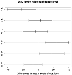
(a) CSR clutter: P${}={}$154.36,	(b) Inhomogeneous Poisson clutter: P${}={}$155.46,
L${}={}$175.93, V${}={}$178.93, W${}={}$172.22	L${}={}$170.40, V${}={}$188.96, W${}={}$173.60
(c) Matérn clutter: P${}={}$150.59,	(d) Thomas clutter: P${}={}$143.09,
L${}={}$173.23, V${}={}$184.39, W${}={}$171.21	L${}={}$176.15, V${}={}$181.48, W${}={}$177.56

Figure 6: The 95% family-wise confidence intervals on the mean differences in traversal lengths based on Tukey’s HSD method for the best performing obstacle type-obstacle number combinations (written as obs. form) at each background clutter type. The average travel lengths for each obstacle form is also provided below the figures.

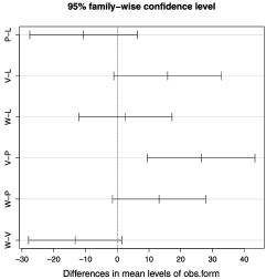
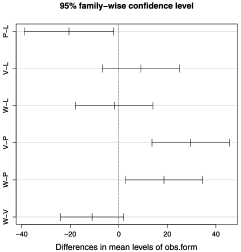
(e) Hardcore clutter: P${}={}$163.86,	(f) Strauss clutter: P${}={}$158.94,
L${}={}$174.43, V${}={}$190.29, W${}={}$177.04	L${}={}$179.45, V${}={}$188.56, W${}={}$177.56

Figure 6: (Continued).

The longest traversal lengths (that are significantly larger than the others) at each clutter type among the best performers are marked in bold face in Table 2. For each clutter type, we compare the mean traversal lengths of the best performer obstacle type-obstacle number combinations by Tukey’s HSD (honestly significant difference) method on mean differences [Miller (1981)]. The corresponding 95% family-wise confidence intervals (CI) are plotted in Figure 6, where the intervals that intersect the vertical line at zero indicate that the corresponding treatments are not significantly different at the 0.05 level. Best performers for each clutter type are described below.

CSR clutter: The longest lengths (that are significantly larger than others) among best performers (in decreasing order) are at V-shaped, linear and W-shaped obstacle forms. That is, the lengths for the V-shaped, linear and W-shaped best performers are not significantly different from each other at the 0.05 level, although the mean difference between V-shaped and W-shaped best performers has $p$-value 0.0645. Hence, for the CSR clutter, we recommend the use of V80:50, V50:40, V70:50 or L20:50 obstacle type in this order. That is, if the cost of the above obstacle placements is about the same, then any one of them can be used, but V80:50 has a slight advantage, otherwise the one with the lowest cost is recommended.

Inhomogeneous Poisson clutter: The longest length among best performers is at V-shaped obstacle forms. Hence, V90:60 obstacle type is recommended.

Matérn clutter: The longest length among best performers is at V-shaped obstacle forms. Hence, V90:50 obstacle type is recommended.

Thomas clutter: The longest lengths among best performers (in decreasing order) are at V-shaped, W-shaped and linear obstacle forms. That is, the lengths for the V-shaped, W-shaped and linear best performers are not significantly different from each other at the 0.05 level. Hence, V90:60, W60:60 or L20:50 obstacle types are recommended in this order. If there are no cost restrictions, V90:60 has a slight advantage, otherwise the one with cheapest construction can be employed.

Hardcore clutter: The longest length among best performers is at V-shaped obstacle forms. Hence, V90:50 obstacle type is recommended.

Strauss clutter: The longest lengths among best performers (in decreasing order) are at V-shaped and linear obstacle forms, although the mean difference between V-shaped and linear best performers has $p$-value 0.0745. Hence, V80:40 or V90:50 obstacle types are recommended in this order as in the previously discussed sense.

Table 4: Cross-tabulation of best performers among obstacle types for clutter type-obstacle number combinations. The corresponding mean traversal lengths are provided in parentheses

	Obstacle number
Clutter	20	30	40	50	60
CSR	L20 (147.92)	L20 (171.57)	V70 (177.02)	V70 (178.68)	V90 (177.02)
			V80 (177.84)	V80 (179.12)
			V50 (178.98)
Inhom.	L30 (151.74)	V60 (167.72)	V60 (175.72)	V90 (184.44)	V90 (188.96)
Poisson		L30 (168.29)
		L40 (168.85)
Matérn	L20 (139.07)	L20 (163.10)	L20 (173.23)	V90 (184.39)	V90 (177.55)
		L30 (164.52)
Thomas	L20 (141.19)	L20 (166.20)	V70 (178.57)	V50 (179.40)	V90 (181.48)
Hardcore	L40 (156.27)	L20 (179.43)	V80 (187.57)	V90 (190.29)	V60 (180.44)
Strauss	L60 (143.81)	L20 (177.31)	V80 (188.77)	V90 (188.35)	V80 (180.37)
	L50 (144.97)

We also provide a cross-tabulation of best performer obstacle type for each clutter type-obstacle number combination in Table 4. For example, for the Matérn clutter with 40 obstacles, the highest traversal length occurs for L20 obstacle pattern. That is, when we know that the clutter is of Matérn type and has only 40 obstacles, the optimal strategy is to employ L20 obstacle scheme. However, if obstacle number is not restricted (i.e., 60 or more), the optimal choice is V90 obstacle scheme.

7 Example data: Maritime minefield application

7.1 Data description

Maritime minefield detection, localization and navigation have received considerable attention from scientific and engineering communities recently; see, for example, Witherspoon et al. (1995), Muhandiramge (2008) and the references cited therein. Operational concepts for maritime minefield detection via unmanned aerial vehicles are discussed in Witherspoon et al. (1995) wherein multi-spectral imagery of a potential minefield is examined and locations of potential mines are identified using a classification algorithm. Of particular interest is a U.S. Navy minefield data set (called the COBRA data) that first appeared in Witherspoon et al. (1995) and was later referred to in Priebe, Olson and Healy (1997), Priebe et al. (2005), Fishkind et al. (2007), Ye and Priebe (2010), Ye, Fishkind and Priebe (2011), and Aksakalli et al. (2011). The COBRA data, illustrated in Figure 7(a), has a total of 39 disk-shaped potential mines of which 27 are clutter and the remaining 12 are true mines [Ye, Fishkind and Priebe (2011)]. The original data coordinates were scaled and shifted so that clutter disk centers are inside the region $[10,90]\times[10,90]$. As in our simulations, we take $s=(50,100)$ and $t=(50,1)$, disk radius as $r=4.5$, and cost of disambiguation as $c=5$ (our simulation environment was in fact inspired by the COBRA data). When the ARD algorithm is applied on the COBRA data [shown in Figure 7(b)], the actual traversal length is 111.46 units with one disambiguation.

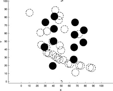
(a) Actual status of the minefield

(b) The minefield as seen by the NAVA and its traversal

Figure 7: The COBRA data and the NAVA’s traversal using the ARD algorithm. Figure (a) shows the actual allocation of the minefield where clutter disks are denoted by dashed circles and mines are denoted by black disks. Figure (b) depicts the COBRA minefield as seen by the NAVA and its $s-t$ traversal.

Figure 8: Plots for mean traversal lengths for the 19 obstacle types (left) and 4 obstacle forms (right) with 12 mines and the 27 COBRA clutter disks. The horizontal dashed line is at 111.46 which is the traversal length for the 12 mines as originally placed in the COBRA data.

A visual inspection of the COBRA clutter suggests that it does not seem to fit any one of the six clutter distribution types considered in this work. Instead, in the scaled coordinates, the pattern looks like a realization from an inhomogeneous Poisson process with intensity being inversely proportional to the distance to the diagonal line, $y=-x+100$. That is, the clutter is more concentrated around this line, compared to regions further away.

7.2 Analysis of traversal lengths for the example data with 12 mines

In this section we investigate whether placing the 12 mines in our example data set using any one of our 19 obstacle placing schemes results in longer traversal lengths compared to their actual placements. Using the 19 obstacle schemes from 4 obstacle forms we consider, mean traversal lengths are plotted in Figure 8 with 100 realizations from each scheme. The shortest traversal lengths occur at W and P obstacle forms with traversal length 112.1, and the highest traversal lengths occur at linear obstacle type L20 with traversal length 114.60. While the difference is not drastic, it is a better strategy on the average to use the L20 obstacle placing scheme to place these 12 mines compared to their original allocation in the COBRA data. Since we are using the same (COBRA) clutter realization for each of 1900 Monte Carlo replications, the setting does not lend itself for repeated measures ANOVA. There seems to be a dependence between traversal length measurements, but since the same clutter is used for each realization, it is as if the same subject receives all 1900 realizations of treatments. Hence, we use the usual ANOVA in our subsequent analysis. The ANOVA assumptions are the same as the repeated measures ANOVA with compound symmetry having zero covariance. We also find significant differences in mean traversal lengths among the obstacle types ($p<0.0001$) and the obstacle forms ($p<0.0001$). Mean traversal lengths are significantly different for the 5 obstacle types among the W-shaped obstacle form ($p=0.0303$). However, mean traversal lengths are not significantly different for the 8 obstacle types among the linear obstacle form ($p=0.1287$) nor the 5 obstacle types among the V-shaped obstacle forms ($p=0.1931$).

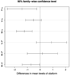
Figure 9: The 95% family-wise confidence intervals on the mean differences in traversal lengths based on Tukey’s HSD method for the obstacle types with the COBRA clutter. The mean traversal lengths for the treatment combinations are P${}={}$112.08, W${}={}$112.26, V${}={}$112.96 and L${}={}$113.50.

We now compare the mean traversal lengths for the obstacle forms by Tukey’s HSD method on mean differences. The corresponding 95% family-wise confidence intervals are plotted in Figure 9. We observe that mean traversal lengths are not significantly different for linear and V-shaped obstacle forms ($p=0.1363$), but linear form is significantly better than the P obstacle form ($p=0.0087$) and W-shaped obstacle form ($p<0.0001$). The P obstacle form is not significantly different from the V-shaped form ($p=0.2127$) nor from the W-shaped form ($p=0.9793$). On the other hand, the V-shaped obstacle form is significantly better than the W-shaped form ($p=0.0378$).

We also experiment with our 19 obstacle placement schemes with a different number of mines (ranging from 20 to 60 in 10 unit increments) to gain insight into which scheme(s) perform better for the example (COBRA) data clutter disks. Again, since we are using the same COBRA clutter as the background pattern for each Monte Carlo realization of obstacle type-obstacle number combination, we use the usual ANOVA in our analysis.

7.3 Overall comparison of traversal lengths for the example data

We first consider the following model:

$$T_{ijk}=\mu_{0}+\mu^{O}_{i}+\mu^{\mathrm{NO}}_{j}+\mu^{O,\mathrm{NO}}_{i,j}+\varepsilon_{ijk},$$ (3)

where $\mu_{0}$ is the overall mean, $\mu^{O}_{i}$ is the mean for obstacle type $i$, $\mu^{\mathrm{NO}}_{j}$ is the mean for obstacle number level $j$, $\mu^{O,\mathrm{NO}}_{i,j}$ is the mean for the obstacle type $i$ and obstacle number level $j$ combination (which stands for the interaction between these factors), $T_{ijk}$ is the $k$th traversal length for obstacle type $i$ and obstacle number level $j$, and $\varepsilon_{ijk}$ is the error term with $i=1,2,\ldots,19$, $j=1,2,\ldots,5$, and $k=1,2,\ldots,100$. We find significant interaction between obstacle type and obstacle number levels ($p<0.0001$), and between obstacle form and obstacle number levels ($p<0.0001$), which means the trends in mean lengths plotted in Figure 10 are significantly nonparallel. Hence, it is not reasonable to compare the mean traversal lengths for obstacle types/forms and obstacle number levels (i.e., for the main effects of obstacle type/forms and obstacle numbers), but instead, for example, it will make sense to compare the mean length values for obstacle number levels at each obstacle type or form.

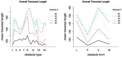
Figure 10: The profile plots for obstacle type/form versus obstacle number for the example clutter pattern.

Table 5: The shortest and longest traversal lengths and the correspondingtreatment types for overall comparisons, and comparisonsat specific clutter types, obstacle types and obstacle numbers

	Shortest		Longest
	Traversal	Treatment	Traversal	Treatment
	length (s)	type (s)	length (s)	type (s)
Overall
	113.03, 113.21,	P:20, W70:20,	176.99	V90:50
	113.76	W50:20
Obstacle form
P	113.03	20	126.07, 127.65	50, 60
Linear	120.40, 120.94	L90:20, L80:20	172.56	L20:50
V-Shaped	114.88	V80:20	176.99	V90:50
W-Shaped	113.21, 113.76	W70:20, W50:20	159.00	W90:60
Number of obstacles
20	113.03, 113.21,	P, W70,	129.54	L20
	113.76	W50
30	116.10, 116.52	P, W70,	162.97	L20
	117.47	W90
40	123.54, 124.38	P, W90	168.91	L20
50	126.07	P	176.99	V90
60	127.67	P	170.02, 171.92	V80, V90

The trend in traversal lengths as number of mines increases is similar to our simulation results. At P and W-shaped obstacle forms, traversal lengths tend to increase as the obstacle number increases. On the other hand, at linear and V-shaped obstacle forms, traversal lengths exhibit a concave-down trend. For linear windows, the shortest length occurs at 20 mines and the longest occurs at 50 mines. For V-shaped windows, shortest length occurs at 20 mines, and longest length occurs at 50 mines. For 20–30 mines, the longest traversal lengths occur at linear obstacle forms, and for 40–60 mines, the longest lengths occur at V-shaped obstacle forms.

The shortest and longest traversal length performances are presented in Table 5. Overall, the shortest length is about 113 units which occurs at P:20, W70:20 and W50:20 treatment combinations, and the longest length is about 177 which occurs at V90:50 treatment combination.

7.4 Analysis of traversal lengths at each obstacle form for the example data

We now investigate the interaction between obstacle type and obstacle number at each obstacle form. Note that no interaction is well defined for the P obstacle form. For other obstacle forms such interaction is possible. In Figure 11 we present the profile plots for interaction between obstacle type and obstacle number at each obstacle form (other than the P obstacle form).

At the P obstacle form, we consider the following model:

$$T_{1jk}=\mu_{0}+\mu^{O}_{1}+\mu^{\mathrm{NO}}_{j}+\varepsilon_{1jk}.$$ (4)

At other obstacle forms, we consider the following model:

$$T_{ijk}=\mu_{0}+\mu^{O}_{i}+\mu^{\mathrm{NO}}_{j}+\mu^{O,\mathrm{NO}}_{i,j}+\varepsilon_{ijk},$$ (5)

where obstacle form indices $j=2,3,4$ stand for linear, V-shaped and W-shaped obstacle forms, respectively.

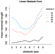
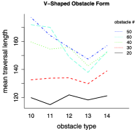
(a)	(b)

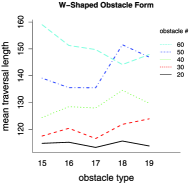
(c)

Figure 11: The profile plots for obstacle type versus obstacle number level at obstacle forms other than P.

The P obstacle form: The traversal lengths are significantly different between obstacle number levels ($p<0.0001$).

Linear obstacle form: We find significant interaction between obstacle type and obstacle number levels ($p<0.0001$). Hence, the trends in mean lengths plotted in Figure 11(a) are significantly different from being parallel. So, it is not reasonable to test for the main effects of obstacle types or obstacle number levels at the linear obstacle form.

V-shaped obstacle form: We find significant interaction between obstacle type and obstacle number levels ($p<0.0001$). Hence, the corresponding trends in mean length plotted in Figure 11(b) are significantly nonparallel. So, it is not reasonable to compare the main effects of obstacle types and obstacle number levels.

W-shaped obstacle form: We find significant interaction between obstacle type and obstacle number levels ($p=0.0004$). Hence, the corresponding trends in mean length plotted in Figure 11(c) are significantly nonparallel. So, it is not reasonable to compare the main effects of obstacle type and obstacle number levels here.

Analysis of traversal lengths for each obstacle form is given below. The shortest and longest traversal lengths together with the corresponding treatment combinations are presented in Table 5.

The P obstacle form: The shortest length is about 113 which occurs at 20 mines, and the longest length is about 127 which occurs at (50 or 60) mines. On the average, traversal lengths tend to increase as the obstacle number increases.

Linear obstacle form: The shortest length is about 120 which occurs at L90:20 and L80:20 treatment types, and the longest length is about 173 which occurs at L20:50 treatment type. At each obstacle type, the shortest lengths occur at 20 obstacles and the highest lengths tend to occur at 50 obstacles. For 20 mines, as the obstacle type level increases from 2 to 9 (i.e., as distance to coast decreases), mean traversal length tends to increase slightly. However, for other mine number levels, the trend exhibits a concave-up behavior (i.e., first decreases, reaches a minimum and then increases).

V-shaped obstacle form: The shortest length is about 115 which occurs at V80:20 treatment type, and the longest length is about 177 which occurs at V90:50 treatment type. As the V-shaped pattern changes from 10–14 (i.e., as distance to coast decreases), the traversal lengths tend to stay stable for 20–30 mines, but for 40–60 mines, it follows a concave-up behavior.

W-shaped obstacle form: The shortest length is about 113 which occurs at W70:20, W50:20 treatment types, and the longest length is about 159 which occurs at W90:60 treatment type. Traversal lengths tend to stay stable for 20–40 mines, but for 50 mines it exhibits a concave-down behavior, and for 60 mines a concave-up behavior.

7.5 Analysis of traversal lengths at each obstacle number level for the example data

We also investigate the relation between traversal lengths and obstacle type/form at each obstacle number level. At each obstacle number level, we consider a model as in equation (3). For example, with 20 obstacles, the model is

$$T_{i1k}=\mu_{0}+\mu^{O}_{i}+\mu^{\mathrm{NO}}_{1}+\varepsilon_{i1k}.$$ (6)

Comparison of traversal lengths for each number of obstacles is presented below. The shortest and longest traversal lengths together with the corresponding treatment combinations are presented in Table 1.

For 20 mines, the shortest traversal length is about 113 which occurs at P, W70, W50 treatment types, and the longest length is about 129 which occurs at L20 treatment type. For 30 mines, the shortest length is about 116 which occurs at P, W70, W90 treatment types, and the longest length is about 163 which occurs at L20 treatment type. For 40 mines, the shortest length is about 124 which occurs at P, W90 treatment types, and the longest length is about 168 which occurs at L20 treatment type. For 50 mines, the shortest length is about 126 which occurs at P treatment type, and the longest length is about 177 which occurs at V90 treatment type. For 60 mines, the shortest length is about 128 which occurs at P treatment type, and the longest length is about 171 which occurs at V80, V90 treatment types.

For 20 and 30 mines, on the average, the longest travel lengths occur for the linear obstacle form. On the other hand, for 40–60 mines, the longest traversal lengths occur for the V-shaped obstacle form. For 20–60 mines, the shortest lengths occur for the P obstacle form. Furthermore, for 20–60 mines, the traversal lengths have a concave-up trend as distance to coast decreases.

7.6 Comparison of best performers for the example data

The overall best performer and best performers for each obstacle type are presented in Table 5. Since there are multiple best performer obstacle type-obstacle number combinations, we compare the traversal lengths for obstacle form levels. We consider the following model:

$$T_{ij}=\mu_{0}+\mu^{\mathrm{OF}}_{i}+\varepsilon_{ij},$$ (7)

where $\mu_{0}$ is the overall mean, $\mu^{\mathrm{OF}}_{i}$ is the main effect of obstacle form $i$, and $\varepsilon_{ij}$ is the error term for $i=1,2,3,4$ (which correspond to P, linear, V-shaped and W-shaped obstacle forms) and $j=1,2,\ldots,n_{i}$, where $n_{i}$ is $k\times 100$ with $k$ being the number of treatment combinations that are best performers. For example, $k=2$ for the P obstacle type.

Figure 12: The 95% family-wise confidence intervals on the mean differences in traversal lengths based on Tukey’s HSD method for the best performing obstacle type-obstacle number combinations at each background clutter type. The mean traversal lengths for the treatment combinations are P${}={}$126.86, L${}={}$172.56, V${}={}$176.99 and W${}={}$159.00.

We compare the mean traversal lengths of the best performer obstacle type-obstacle number combinations by Tukey’s HSD method on mean differences. The corresponding 95% family-wise confidence intervals are plotted in Figure 12. Notice that best performers for linear and V-shaped obstacle forms are not significantly different ($p=0.8148$), but the V-shaped is significantly larger than P ($p<0.0001$) and W-shaped obstacle forms ($p=0.0021$). Furthermore, the linear is also significantly larger than P ($p<0.0001$) and W-shaped obstacle forms ($p=0.0358$). Finally, the W-shaped form is significantly larger than the P obstacle form ($p<0.0001$).

8 Discussion and conclusions

In this work we introduce the obstacle placement with the disambiguations (OPD) problem wherein the objective is to place a given number of true obstacles in between the clutter so as to maximize the traversal length of the navigating agent (NAVA) in a game-theoretic sense. We consider a specific version of the problem where the obstacle placing agent (OPA) knows the clutter type (i.e., the clutter spatial distribution), but not the exact location of clutter disks. We investigate relative efficiency of a variety of obstacle placement patterns against different background clutter types. Our goal is to explore the effect of the number of obstacles on the NAVA’s traversal length and to determine which obstacle placement patterns perform better for a given clutter type. We also present an extensive case study on a real-world maritime minefield data set. We believe that such an analysis within a maritime minefield context has a significant potential in the design of more efficient and cost-effective interdiction systems.

Our setup leads to a three-way repeated measures ANOVA problem where the treatment factors are the clutter type, number of obstacles and the obstacle placement pattern, with the response variable being the NAVA’s total traversal length. We choose repeated measures ANOVA instead of the usual ANOVA to gain more precision and power in our analysis. Furthermore, the model assumptions for repeated measures ANOVA are satisfied with the flexibility of modeling different types of correlation between repeated measures. We consider a total of 6 clutter types: homogeneous Poisson process (also known as CSR), inhomogeneous Poisson process, Matérn, Thomas, hard-core and Strauss point processes. We consider 5 different numbers of obstacles (20, 30$,\ldots,$60), and we experiment with a total of 19 different obstacle placement patterns sampled from CSR in four different forms: the clutter sampling window $P$, linear, V- and W-shaped polygon windows.

Extensive statistical analysis of our Monte Carlo simulations indicate that as the clutter spatial distribution becomes more regular (clustered), the traversal length gets longer (shorter). In terms of obstacle number levels, the traversal length tends to follow a concave-down trend (i.e., increases, reaches a peak and then decreases) as the number of obstacles increases. The reason for the traversal trend following such a concave-down trend is that the traversal length tends to increase to a certain extent as the hindrance disk (obstacle${}+{}$clutter) density increases, reaches an optimum and then decreases, as the NAVA tends to avoid the obstacle window altogether when the hindrance density becomes too high. This is perhaps a counterintuitive result at first, as placing more and more obstacles in the obstacle field becomes detrimental after a certain point from the OPA’s perspective.

In terms of obstacle forms, the shortest traversals tend to occur for the P obstacle form. The longest traversal lengths, on the other hand, tend to occur for the V-shaped obstacle form. It appears that the V-shaped obstacle form tends to trap the NAVA within its elbow like (convex) region, especially in the presence of a large number of obstacles. Under CSR clutter, linear obstacle forms enjoy the longest traversal for small obstacle numbers (20–30), and V-shaped obstacle forms enjoy the longest traversal for moderate to large obstacle numbers (40–60). For other clutter types, the V-shaped obstacle form that is closer to the starting point with a large number of obstacles tends to result in the longest traversals. In particular, the longest traversals occur at V90:60 for the CSR and Thomas clutter types; V90:50 for Matérn, hardcore, and Strauss clutter types; and V70:50 for the inhomogeneous Poisson clutter type. Among linear obstacle forms, the traversal tends to get longer as the linear obstacle window gets closer to the target, while among V- and W-shaped obstacle forms traversal tends to get longer as the obstacle window gets further away from the target. Thus, with a small number of obstacles (i.e., 20–30 obstacles), the best performers are linear obstacle windows closer to the target. As for larger obstacle numbers (i.e., 40–60 obstacles), the best performers are V-shaped obstacle windows closer to the starting point.

Our results and conclusions are valid only for the specific experimental setup we consider, so they are likely to change for different clutter and/or obstacle windows, mark distribution, disambiguation cost or clutter type parameters. Nonetheless, the statistical analysis we present in this study can easily be adapted to analyze OPD problem instances within such different environments. In fact, we also study a real-world maritime minefield data set with 27 clutter and 12 actual obstacles (see Section 7). Even though the real-world clutter pattern does not resemble any of the clutter patterns we consider in our simulations, analysis of our obstacle placement schemes for the real-world clutter results in a similar conclusion as our Monte Carlo simulations: for smaller obstacle numbers, larger traversal lengths occur for linear obstacle forms closer to the target, and for moderate-to-larger obstacle numbers, larger traversal lengths occur for V-shaped obstacle forms closer to the starting point. In what follows, we provide a brief discussion on several issues related to our research.

Asymmetry of information: An inherent assumption in our framework is asymmetry of information between the NAVA and the OPA: it is assumed that the OPA knows the distribution of the clutter whereas the NAVA does not. On the other hand, should the NAVA have certain prior information on clutter distribution, it can incorporate this information into its traversal strategy by updating disk marks accordingly. Specifically, the NAVA can assign lower marks to disks fitting the overall clutter pattern while assigning higher marks to disks that do not (perhaps when considered in conjunction with spectral image properties of the disks). Thus, our framework allows for incorporation of any information on clutter distribution from the NAVA’s perspective. In fact, our simulation setup can be seen as accounting for this asymmetry of information to a certain extent: clutter marks are sampled from $\operatorname{Beta}(6,2)$ (with a mean of 0.25) whereas obstacle marks are sampled from $\operatorname{Beta}(2,6)$ (with a mean of 0.75).

Sampling obstacle centers from homogeneous Poisson distribution: In our simulations, obstacle disk centers are sampled from a homogeneous Poisson distribution within their respective obstacle windows, potentially resulting in overlapping obstacles. On the other hand, it can be argued that this is not an ideal strategy, as it is more sensible for the OPA to maximize the space occupied by true obstacles. From that perspective, a hardcore process should have been preferred for sampling obstacle disk centers. The reason we chose homogeneous Poisson over hardcore was to keep information asymmetry at a minimum. Specifically, in the case of hardcore obstacle centers, if a disambiguated disk turns out to be a true obstacle, the optimal strategy for the NAVA would be to decrease marks of surrounding disks in some fashion. On the other hand, with a homogeneous Poisson, as in our simulations, learning that a disambiguated disk is a true obstacle does not give the NAVA any additional information regarding the actual status of surrounding disks. The crucial observation here is that the ARD algorithm, as currently implemented, would not have accounted for such mark dependencies had we used hardcore instead of homogeneous Poisson, giving the NAVA an unfair disadvantage. We leave it to future research to adapt the ARD algorithm for such a dependency structure and then use the hardcore pattern for generating obstacle disk centers.

Limitations of the ARD algorithm: The ARD algorithm is currently the state-of-the-art method for optimal navigation in stochastic environments in the presence of a disambiguation capability. On the other hand, it is merely a heuristic method with no guaranteed performance bounds—yet the underlying problem is a challenging stochastic optimization problem and all known exact methods have exponential computational complexity. Our observation that average traversal length tends to be concave-down with respect to the number of obstacles might indeed be attributed to short-comings of the ARD algorithm rather than benefits of fewer obstacles. This issue warrants further investigation of the ARD algorithm’s performance, which is left to future research.

Our work can be extended in several directions. First, more clutter types and various other obstacle placement schemes can be considered. Second, another variant of the OPD problem can be studied where the OPA knows the exact locations of background clutter disks prior to placing the true obstacles. In this particular case, the OPA can strategically place the obstacles (as opposed to placing them randomly inside a predetermined obstacle window). This approach is likely to be more efficient in terms of slowing down the progress of the NAVA. However, as mentioned earlier, one downside of this specific variant is that it requires that the OPA knows the sensor technology of the NAVA, that is, the OPA has information on which specific areas NAVA’s sensors detect as potential obstacle regions. Third, a more general version of the OPD problem can be investigated where the OPA also has control over the clutter disk locations (in addition to the obstacle disk locations). In this version, the OPA’s challenge would be to place a given number of true and false obstacle disks in the field, again so as to maximize the traversal length of the NAVA in a game-theoretic sense.

References

- Aksakalli (2007) {bmisc}[author] \bauthor\bsnmAksakalli, \bfnmV.\binitsV. (\byear2007). \bhowpublishedThe algorithm for stochastic shortest path problems with dynamic learning. In Proceedings of IEEE Conference on Decision and Control, New Orleans. \bptokimsref \endbibitem
- Aksakalli and Ceyhan (2012) {bmisc}[author] \bauthor\bsnmAksakalli, \bfnmV.\binitsV. and \bauthor\bsnmCeyhan, \bfnmE.\binitsE. (\byear2012). \bhowpublishedOptimal obstacle placement with disambiguations. Technical Report #SEHIR-IE-VA-12-1, Istanbul Şehir University, Istanbul 34662, Turkey. Available at arXiv:\arxivurl1201.5076 [stat.AP]. \bptokimsref \endbibitem
- Aksakalli et al. (2011) {barticle}[mr] \bauthor\bsnmAksakalli, \bfnmVural\binitsV., \bauthor\bsnmFishkind, \bfnmDonniell E.\binitsD. E., \bauthor\bsnmPriebe, \bfnmCarey E.\binitsC. E. and \bauthor\bsnmYe, \bfnmXugang\binitsX. (\byear2011). \btitleThe reset disambiguation policy for navigating stochastic obstacle fields. \bjournalNaval Res. Logist. \bvolume58 \bpages389–399. \biddoi=10.1002/nav.20454, issn=0894-069X, mr=2729920 \bptokimsref \endbibitem
- Baddeley (2010) {bmisc}[author] \bauthor\bsnmBaddeley, \bfnmA.\binitsA. (\byear2010). \bhowpublishedAnalysing spatial point patterns in R. Workshop notes Ver. 4.1. \bptokimsref \endbibitem
- Baddeley and Turner (2005) {barticle}[author] \bauthor\bsnmBaddeley, \bfnmA.\binitsA. and \bauthor\bsnmTurner, \bfnmR.\binitsR. (\byear2005). \btitleSpatstat: An R package for analyzing spatial point patterns. \bjournalJournal of Statistical Software \bvolume12 \bpages1–42. \bptokimsref \endbibitem
- Burnham and Anderson (2003) {bbook}[author] \bauthor\bsnmBurnham, \bfnmK. P.\binitsK. P. and \bauthor\bsnmAnderson, \bfnmD.\binitsD. (\byear2003). \btitleModel Selection and Multi-Model Inference. \bpublisherSpringer, \baddressNew York. \bptokimsref \endbibitem
- Cressie (1993) {bbook}[mr] \bauthor\bsnmCressie, \bfnmNoel A. C.\binitsN. A. C. (\byear1993). \btitleStatistics for Spatial Data. \bpublisherWiley, \baddressNew York. \bidmr=1239641 \bptokimsref \endbibitem
- Cressie and Brant Collins (2001) {barticle}[mr] \bauthor\bsnmCressie, \bfnmNoel\binitsN. and \bauthor\bsnmCollins, \bfnmLinda Brant\binitsL. B. (\byear2001). \btitlePatterns in spatial point locations: Local indicators of spatial association in a minefield with clutter. \bjournalNaval Res. Logist. \bvolume48 \bpages333–347. \biddoi=10.1002/nav.1022.abs, issn=0894-069X, mr=1856313 \bptokimsref \endbibitem
- Cressie and Lawson (2000) {barticle}[mr] \bauthor\bsnmCressie, \bfnmNoel\binitsN. and \bauthor\bsnmLawson, \bfnmAndrew B.\binitsA. B. (\byear2000). \btitleHierarchical probability models and Bayesian analysis of mine locations. \bjournalAdv. in Appl. Probab. \bvolume32 \bpages315–330. \biddoi=10.1239/aap/1013540165, issn=0001-8678, mr=1778566 \bptokimsref \endbibitem
- Daley and Vere-Jones (2002) {bbook}[author] \bauthor\bsnmDaley, \bfnmD. J.\binitsD. J. and \bauthor\bsnmVere-Jones, \bfnmD.\binitsD. (\byear2002). \btitleAn Introduction to the Theory of Point Processes, \bedition2nd ed. \bpublisherSpringer, \baddressNew York. \bptokimsref \endbibitem
- Eyerich, Keller and Helmert (2009) {bmisc}[author] \bauthor\bsnmEyerich, \bfnmP.\binitsP., \bauthor\bsnmKeller, \bfnmT.\binitsT. and \bauthor\bsnmHelmert, \bfnmM.\binitsM. (\byear2009). \bhowpublishedHigh-quality policies for the Canadian traveler’s problem. In Proceedings of the 24th AAAI Conference on Artificial Intelligence, Atlanta, Georgia. \bptokimsref \endbibitem
- Fishkind et al. (2007) {barticle}[author] \bauthor\bsnmFishkind, \bfnmD. E.\binitsD. E., \bauthor\bsnmPriebe, \bfnmC. E.\binitsC. E., \bauthor\bsnmGiles, \bfnmK.\binitsK., \bauthor\bsnmSmith, \bfnmL. N.\binitsL. N. and \bauthor\bsnmAksakalli, \bfnmV.\binitsV. (\byear2007). \btitleDisambiguation protocols based on risk simulation. \bjournalIEEE Transactions on Systems, Man, and Cybernetics, Part A \bvolume37 \bpages814–823. \bptokimsref \endbibitem
- Howell (2010) {bbook}[author] \bauthor\bsnmHowell, \bfnmD. C.\binitsD. C. (\byear2010). \btitleFundamental Statistics for the Behavioral Sciences. \bpublisherWadsworth Publishing, \baddressBelmont, CA. \bptokimsref \endbibitem
- Kuehl (2000) {bbook}[author] \bauthor\bsnmKuehl, \bfnmR. O.\binitsR. O. (\byear2000). \btitleDesign of Experiments: Statistical Principles of Research Design and Analysis, \bedition2nd ed. \bpublisherBrooks/Cole, \baddressPacific Grove, CA. \bptokimsref \endbibitem
- Likhachev and Stentz (2009) {barticle}[mr] \bauthor\bsnmLikhachev, \bfnmMaxim\binitsM. and \bauthor\bsnmStentz, \bfnmAnthony\binitsA. (\byear2009). \btitleProbabilistic planning with clear preferences on missing information. \bjournalArtificial Intelligence \bvolume173 \bpages696–721. \biddoi=10.1016/j.artint.2008.10.014, issn=0004-3702, mr=2504428 \bptokimsref \endbibitem
- Miller (1981) {bbook}[mr] \bauthor\bsnmMiller, \bfnmRupert G.\binitsR. G. \bsuffixJr. (\byear1981). \btitleSimultaneous Statistical Inference, \bedition2nd ed. \bpublisherSpringer, \baddressNew York. \bidmr=0612319 \bptokimsref \endbibitem
- Møller and Waagepetersen (2007) {barticle}[mr] \bauthor\bsnmMøller, \bfnmJesper\binitsJ. and \bauthor\bsnmWaagepetersen, \bfnmRasmus P.\binitsR. P. (\byear2007). \btitleModern statistics for spatial point processes. \bjournalScand. J. Stat. \bvolume34 \bpages643–684. \biddoi=10.1111/j.1467-9469.2007.00569.x, issn=0303-6898, mr=2392447 \bptokimsref \endbibitem
- Muhandiramge (2008) {bmisc}[author] \bauthor\bsnmMuhandiramge, \bfnmR.\binitsR. (\byear2008). \bhowpublishedMaritime manoeuvring optimization: Path planning in minefield threat environments. Ph.D. thesis, Univ. Western Australia. \bptokimsref \endbibitem
- Muise and Smith (1995) {barticle}[author] \bauthor\bsnmMuise, \bfnmR. R.\binitsR. R. and \bauthor\bsnmSmith, \bfnmC. M.\binitsC. M. (\byear1995). \btitleA linear density algorithm for patterned minefield detection. \bjournalProceedings of the SPIE \bvolume2496 \bpages586–593. \bptokimsref \endbibitem
- Nikolova and Karger (2008) {bmisc}[author] \bauthor\bsnmNikolova, \bfnmE.\binitsE. and \bauthor\bsnmKarger, \bfnmD. R.\binitsD. R. (\byear2008). \bhowpublishedRoute planning under uncertainty: The Canadian traveller problem. In Proceedings of the 23rd AAAI Conference on Artificial Intelligence, Chicago, Illinois. \bptokimsref \endbibitem
- Olson, Pang and Priebe (2003) {barticle}[mr] \bauthor\bsnmOlson, \bfnmTim\binitsT., \bauthor\bsnmPang, \bfnmJong-Shi\binitsJ.-S. and \bauthor\bsnmPriebe, \bfnmCarey\binitsC. (\byear2003). \btitleA likelihood-MPEC approach to target classification. \bjournalMath. Program. \bvolume96 \bpages1–31. \biddoi=10.1007/s10107-003-0242-8, issn=0025-5610, mr=1974165 \bptokimsref \endbibitem
- Papadimitriou and Yannakakis (1991) {barticle}[mr] \bauthor\bsnmPapadimitriou, \bfnmChristos H.\binitsC. H. and \bauthor\bsnmYannakakis, \bfnmMihalis\binitsM. (\byear1991). \btitleShortest paths without a map. \bjournalTheoret. Comput. Sci. \bvolume84 \bpages127–150. \biddoi=10.1016/0304-3975(91)90263-2, issn=0304-3975, mr=1122649 \bptokimsref \endbibitem
- Pinheiro and Bates (2000) {bbook}[author] \bauthor\bsnmPinheiro, \bfnmJ. C.\binitsJ. C. and \bauthor\bsnmBates, \bfnmD. M.\binitsD. M. (\byear2000). \btitleMixed-Effects Models in S and S-PLUS. \bpublisherSpringer, \baddressNew York. \bptokimsref \endbibitem
- Priebe, Olson and Healy (1997) {barticle}[author] \bauthor\bsnmPriebe, \bfnmC. E.\binitsC. E., \bauthor\bsnmOlson, \bfnmT. E.\binitsT. E. and \bauthor\bsnmHealy, \bfnmD. M.\binitsD. M. (\byear1997). \btitleExploiting stochastic partitions for minefield detection. \bjournalProceedings of the SPIE \bvolume3079 \bpages508–518. \bptokimsref \endbibitem
- Priebe et al. (2005) {barticle}[mr] \bauthor\bsnmPriebe, \bfnmCarey E.\binitsC. E., \bauthor\bsnmFishkind, \bfnmDonniell E.\binitsD. E., \bauthor\bsnmAbrams, \bfnmLowell\binitsL. and \bauthor\bsnmPiatko, \bfnmChristine D.\binitsC. D. (\byear2005). \btitleRandom disambiguation paths for traversing a mapped hazard field. \bjournalNaval Res. Logist. \bvolume52 \bpages285–292. \biddoi=10.1002/nav.20071, issn=0894-069X, mr=2135903 \bptokimsref \endbibitem
- Provan (2003) {barticle}[mr] \bauthor\bsnmProvan, \bfnmJ. Scott\binitsJ. S. (\byear2003). \btitleA polynomial-time algorithm to find shortest paths with recourse. \bjournalNetworks \bvolume41 \bpages115–125. \biddoi=10.1002/net.10063, issn=0028-3045, mr=1959091 \bptokimsref \endbibitem
- Rippley (2004) {bbook}[author] \bauthor\bsnmRippley, \bfnmB. D.\binitsB. D. (\byear2004). \btitleSpatial Statistics. \bpublisherWiley, \baddressHoboken, NJ. \bptokimsref \endbibitem
- Tabachnick and Fidell (2006) {bbook}[author] \bauthor\bsnmTabachnick, \bfnmG. G.\binitsG. G. and \bauthor\bsnmFidell, \bfnmL. S.\binitsL. S. (\byear2006). \btitleExperimental Designs Using ANOVA. \bpublisherDuxbury, \baddressBelmont, CA. \bptokimsref \endbibitem
- Walsh and Raftery (2002) {barticle}[mr] \bauthor\bsnmWalsh, \bfnmDaniel C. I.\binitsD. C. I. and \bauthor\bsnmRaftery, \bfnmAdrian E.\binitsA. E. (\byear2002). \btitleDetecting mines in minefields with linear characteristics. \bjournalTechnometrics \bvolume44 \bpages34–44. \biddoi=10.1198/004017002753398308, issn=0040-1706, mr=1963255 \bptokimsref \endbibitem
- Witherspoon et al. (1995) {barticle}[author] \bauthor\bsnmWitherspoon, \bfnmN. H.\binitsN. H., \bauthor\bsnmHolloway, \bfnmJ. H.\binitsJ. H., \bauthor\bsnmDavis, \bfnmK. S.\binitsK. S., \bauthor\bsnmMiller, \bfnmR. W.\binitsR. W. and \bauthor\bsnmDubey, \bfnmA. C.\binitsA. C. (\byear1995). \btitleThe coastal battlefield reconnaissance and analysis (COBRA) program for minefield detection. \bjournalProceedings of the SPIE \bvolume2496 \bpages500–508. \bptokimsref \endbibitem
- Xu et al. (2009) {barticle}[mr] \bauthor\bsnmXu, \bfnmYinfeng\binitsY., \bauthor\bsnmHu, \bfnmMaolin\binitsM., \bauthor\bsnmSu, \bfnmBing\binitsB., \bauthor\bsnmZhu, \bfnmBinhai\binitsB. and \bauthor\bsnmZhu, \bfnmZhijun\binitsZ. (\byear2009). \btitleThe Canadian traveller problem and its competitive analysis. \bjournalJ. Comb. Optim. \bvolume18 \bpages195–205. \biddoi=10.1007/s10878-008-9156-y, issn=1382-6905, mr=2524772 \bptokimsref \endbibitem
- Ye, Fishkind and Priebe (2011) {barticle}[author] \bauthor\bsnmYe, \bfnmX.\binitsX., \bauthor\bsnmFishkind, \bfnmD. E.\binitsD. E. and \bauthor\bsnmPriebe, \bfnmC. E.\binitsC. E. (\byear2011). \btitleSensor information monotonicity in disambiguation protocols. \bjournalJournal of the Operational Research Society \bvolume62 \bpages142–151. \bptokimsref \endbibitem
- Ye and Priebe (2010) {barticle}[author] \bauthor\bsnmYe, \bfnmX.\binitsX. and \bauthor\bsnmPriebe, \bfnmC. E.\binitsC. E. (\byear2010). \btitleA graph-search based navigation algorithm for traversing a potentially hazardous area with disambiguation. \bjournalInternational Journal of Operations Research and Information Systems \bvolume1 \bpages14–27. \bptokimsref \endbibitem