Hybrid of superconducting quantum interference device and atomic Bose-Einstein condensate: An architecture for quantum information processing

Abstract

A hybrid quantum system is proposed by coupling the internal hyperfine transitions of a trapped atomic Bose-Einstein condensate (BEC) and a superconducting quantum interference device (SQUID) via the macroscopic quantum field of the flux qubit. The presence of the condensate leads to a bosonic enhancement of the Rabi frequency over the otherwise small single-particle magnetic dipole transition matrix elements. This enhancement allows for the possibility to rapidly transfer and store qubit states in the BEC that were originally prepared in the SQUID. The fidelity of this transfer for different states is calculated, and a direct experimental protocol to determine the transfer fidelity by quantum tomography of the BEC qubit is presented.

I Introduction

Hybrid quantum systems, systems composed of two or more distinct quantum mechanical subsystems coupled together, is a rapidly developing area, and a subject that intrinsically spans many disciplines, from basic research to engineering Xiang ; Aspelmeyer . On a fundamental level, such a combined system was used to probe—for the first time—the quantum nature of a nanomechanical oscillator, by coupling it to a superconducting qubit OConnell . These systems have especially become prominent in the quantum computing community, where such combinations can, for example, be used to overcome the opposing requirements for a quantum computer to have both long coherence times and an ease of external manipulation Blais ; Verdu ; Lukin ; Armour ; Nakamura ; Wallraff ; Zhu ; Wu ; Majer ; Cleland ; Rabl ; Brennecke ; Baumann . Frequently, such hybrid systems are not developed as algorithmic units but to perform auxiliary functions, such as memory elements, where qubit states are transferred from one subsystem and stored in another, or as information buses Majer ; Cleland ; Rabl ; Brennecke ; Baumann ; Blencowe .

Here, we propose a novel quantum memory hybrid, where the storage element is potentially capable of possessing second-long coherence times, competing with the recently engineered coherence times of nitrogen-vacancy (NV) centers in diamond, without the use of a dynamical environment-decoupling scheme vanderSar . This hybrid is created by coupling a SQUID, or flux qubit, and the hyperfine states of a trapped atomic Bose-Einstein condensate (BEC). The SQUID allows for the easy preparation and manipulation of qubit states, while the BEC’s hyperfine qubit states can remain coherent for a extremely long time, on the order of seconds. The latter has been recently demonstrated for a BEC cloud trapped near a superconducting waveguide resonator geometry BernonArxiv2013 , further motivating our study into the present hybrid.

The two qubits are electromagnetically coupled together. The radiation emitted by the circulating macroscopic currents of the flux qubit induces atomic transitions of the trapped BEC atoms. For the system considered here, the transitions are dominated by magnetic dipole coupling but, in general could also be electric dipole driven. The hyperfine transitions can in turn excite the qubit states of the SQUID, resulting in the periodic transfer of energy from one subsystem to the other, i.e., the Rabi process, with a period determined by a Rabi frequency $\Omega$. Qubit states initially prepared in the SQUID can be transferred and stored in the BEC. This process is achieved by dynamically bringing the two subsystems into and out of resonance for approximately a half of a Rabi period $\pi/(2\Omega)$.

Present coherence times of flux qubits are on the order of a few microseconds. Depending on the BEC-SQUID separation, the qubit-state-transfer time can be of the same order. But as was recently shown in Ref. Patton2012 , one can still obtain a high transfer fidelity, even in the face of this naively unfavorable condition.

In the following sections each qubit subsystem will be introduced, starting with the SQUID in Sec. II, followed by the hyperfine qubit in Sec. III, and then the qubit-qubit coupled hybrid system is presented in Sec. IV. Finally, in Secs. V and VI the transfer and storage fidelity is calculated for various qubit states, and an experimental technique is put forward to determine the hyperfine qubit density matrix by quantum tomography.

II Flux qubit

Although the derivation of the effective low-energy Hilbert space of a SQUID can be commonly found in the literature SQUIDHandbook , starting from a quantum circuit model, which is used here, or from a microscopic approach Ambegaokar1982 , several details relevant to the BEC-SQUID coupling are typically not prominently discussed, such as defining a macroscopic current operator for the SQUID and the resulting quantum mechanical electromagnetic fields. Therefore, to make the paper sufficiently self-contained a short review is included here.

For simplicity and clarity, in the following the SQUID is assumed to be a simple rf SQUID, containing a single Josephson tunneling junction, see Fig. 1. The outcome is not dependent on this, and the intermediate details can be readily generalized to other more complex SQUID architectures.

II.1 Quantum circuit model for a SQUID

The supercurrent $I_{\rm s}$ through a weak-link tunneling junction is given by the DC Josephson relation,

$$I_{\rm s}=I_{\rm c}\sin\delta,$$ (1)

where $I_{\rm c}$ is the critical current of the junction, which depends on the microscopic details of the barrier, and $\delta$ is the gauge-invariant phase difference of the superconducting states on each side of the tunneling barrier. Additionally, the voltage across the tunnel junction is related to the time-rate change of the phase difference by Josephson’s second relation

$$V(t)=\frac{\hbar}{2\rm{e}}\frac{d\delta}{dt}=\frac{\Phi_{0}}{2\pi}\frac{d\delta}{dt},$$ (2)

where $\Phi_{0}=\frac{h}{2\rm{e}}$ is the quantum of magnetic flux. The total flux $\Phi$ through the SQUID loop and the phase are related by the flux quantization condition

$$\Phi+\Phi_{0}\delta/(2\pi)=n\Phi_{0},$$ (3)

with $n\in\mathbb{Z}$. The Josephson relations, Eqs. (1) and (2), in terms of the flux variable are

$$I_{\rm s} =-I_{\rm c}\sin\left(\frac{2\pi}{\Phi_{0}}\Phi\right),$$ (4a)

$$V =-\frac{d\Phi}{dt}.$$ (4b)

The total flux through the loop is related to the total current $I$ by

$$\Phi=\Phi_{\rm ex}+LI,$$ (5)

where $\Phi_{\rm ex}$ is any applied external flux and $L$ is the geometric inductance of the SQUID.

Using the current-voltage relations for a capacitor $C$, $I=C\partial_{t}V$, Ohm’s law $I=R^{-1}V$, for a resistor $R$, and Eqs. (4), the time-dependent current around the loop of the rf SQUID model shown in Fig. 1 is given by

Figure 1: Schematic of a rf SQUID in an external magnetic field $B_{\rm ex}$. A realistic Josephson junction is modeled by an ideal junction, denoted by the cross, in parallel with a capacitor $C$ and a resistor $R$.

$$I(t)=-I_{\rm c}\sin\left(\frac{2\pi}{\Phi_{0}}\Phi\right)-C\frac{d^{2}\Phi}{dt^{2}}-\frac{1}{R}\frac{d\Phi}{dt}.$$ (6)

Putting the current (6) into (5) leads to an equation of motion for the flux variable given by

$$C\frac{d^{2}\Phi}{dt^{2}}+\frac{1}{R}\frac{d\Phi}{dt}=-\partial_{\Phi}U(\Phi)$$ (7)

where

$$U(\Phi)=\frac{\left(\Phi-\Phi_{\rm ex}\right)^{2}}{2L}-\frac{I_{\rm c}\Phi_{0}}{2\pi}\cos\left(\frac{2\pi}{\Phi_{0}}\Phi\right).$$ (8)

Sometimes it is convenient to express (8) using dimensionless quantities

$$U(\phi)=U_{0}\left[\frac{(2\pi)^{2}\big{(}\phi-\phi_{\rm ex}\big{)}^{2}}{2}-\beta_{L}\cos(2\pi\phi)\right],$$ (9)

where $U_{0}=\Phi^{2}_{0}/(4\pi^{2}L)$, $\beta_{L}=2\pi LI_{\rm c}/\Phi_{0}$ and $\phi$ and $\phi_{\rm ex}$ are in units of $\Phi_{0}$.

Equation (7) is the equation of motion identical to that of a fictitious particle having a mass $C$ in the presence of a damping, or dissipation, $1/R$ term and potential $U(\Phi)$. Ignoring the dissipation term, valid in the $R\to\infty$ limit, a Lagrangian that produces (7) as an equation of motion is

$${\cal L}=\frac{1}{2}C\dot{\Phi}^{2}-U(\Phi).$$ (10)

A Hamiltonian can be constructed from the Lagrangian in the usual way. Defining the flux $\Phi$ as the generalized coordinate, with conjugate momentum $p_{\Phi}=\partial_{\dot{\Phi}}{\cal L}=C\dot{\Phi}$, the Hamiltonian is

$$H =p_{\Phi}\dot{\Phi}-\cal{L}$$

$$=\frac{p^{2}_{\Phi}}{2C}+U(\Phi).$$ (11)

At the classical level, the Poisson bracket of the generalized coordinate $\Phi$ and its conjugate momentum $p_{\Phi}$ is unity. Thus, one can quantize the SQUID Hamiltonian (II.1) by imposing the standard canonical commutations relations, i.e., $p_{\Phi}\rightarrow-i\hbar\partial_{\Phi}$ such that $[\Phi,p_{\Phi}]=i\hbar$. The energy eigenstate of (II.1) $\psi_{n}$ are then functions of the flux variable $\psi_{n}(\Phi)$. In general these eigenstates have to be found numerically, but in some parameter regimes approximate solutions can be constructed. In the next section the approximate qubit states of the SQUID are given.

II.2 Qubit basis

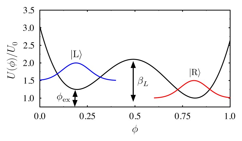
Figure 2: Characteristic potential felt by the fictitious flux particle Eq. (9), where all flux values are in units of the flux quantum, i.e., $\phi=\Phi/\Phi_{0}$, $\beta_{L}=2.1$, and $\phi_{\rm ex}=1.02/2$. The location of the barrier and the asymmetry between the wells is controlled by the external flux $\Phi_{\rm ex}$, while the barrier height is controlled by $\beta_{\rm L}$. For $\beta_{\rm L}=1$ the barrier vanishes. Although in this setup $\beta_{\rm L}$ is fixed, it can be dynamically controlled by introducing additional circuit elements.

A typical plot of the characteristic double well of the effective potential (9) is shown in Fig. 2. For a sufficiently high barrier that separates the two wells one can approximate the low-energy subspace of the Hilbert space, by ground state harmonic oscillators, i.e., Gaussians, centered in each well. These will be labeled as $|{\rm L}\rangle$ and $|{\rm R}\rangle$ and are explicitly given by ($\hbar=1$ in what follows)

$$\langle\Phi|{\rm L}/{\rm R}\rangle=\left(\frac{C\omega_{{\rm L}/{\rm R}}}{\pi}\right)^{1/4}\exp\left[-\frac{C\omega_{{\rm L}/{\rm R}}}{2}\left(\Phi-\Phi^{\rm min}_{{\rm L}/{\rm R}}\right)^{2}\right],$$ (12)

where $\Phi^{\rm min}_{{\rm L}/{\rm R}}$ is the location of the minimum of each well, and $\omega_{{\rm L}/{\rm R}}$ is the effective harmonic frequency of each well. These are related to the full potential (8) by requiring $\partial_{\Phi}U(\Phi^{\rm min}_{{\rm L}/{\rm R}})=0$, such that $\partial^{2}_{\Phi}U(\Phi^{\rm min}_{{\rm L}/{\rm R}})>0$, which implies

$$\Phi^{\rm min}_{{\rm L}/{\rm R}}=\Phi_{\rm ex}-\frac{\Phi_{0}}{2\pi}\beta_{L}\sin\left(\frac{2\pi}{\Phi_{0}}\Phi^{\rm min}_{{\rm L}/{\rm R}}\right),$$ (13)

and

$$\omega_{{\rm L}/{\rm R}} =\sqrt{\partial^{2}_{\Phi}U(\Phi^{\rm min}_{{\rm L}/{\rm R}})/C}$$

$$=\sqrt{\frac{1+\beta_{L}\cos\left(\frac{2\pi}{\Phi_{0}}\Phi^{\rm min}_{{\rm L}/{\rm R}}\right)}{LC}}\sim\sqrt{\frac{1}{LC}}.$$ (14)

Because of the potential offset of each well, controlled by the external flux, see Fig. 2, the ground state energy of each Gaussian is approximately $E_{{\rm L}/{\rm R}}=U(\Phi^{\rm min}_{{\rm L}/{\rm R}})+\omega_{{\rm L}/{\rm R}}+\frac{1}{2}$. For most cases of interest $E_{{\rm L}}-E_{{\rm R}}\approx U(\Phi^{\rm min}_{{\rm L}})-U(\Phi^{\rm min}_{{\rm R}}):=\varepsilon.$

The left-right states are not energy eigenstates. To see this, the SQUID Hamiltonian in this basis is

$$\hat{H} \approx\left(\begin{array}[]{cc}\langle{\rm L}|H|{\rm L}\rangle&\langle{\rm L}|H|{\rm R}\rangle\\ \langle{\rm R}|H|{\rm L}\rangle&\langle{\rm R}|H|{\rm R}\rangle\end{array}\right)\approx\left(\begin{array}[]{cc}E_{\rm L}&-\Delta/2\\ -\Delta/2&E_{\rm R}\end{array}\right)$$ (19)

$$=\frac{E_{\rm L}+E_{\rm R}}{2}\openone+\frac{\varepsilon}{2}\sigma_{z}-\frac{\Delta}{2}\sigma_{x},$$ (20)

where $\Delta$ characterizes the overlap of the left-right states, or tunneling amplitude, and $\sigma_{i}$ are the Pauli matrices. The minus sign in front of the $\sigma_{x}$ term is chosen to give a symmetric lowest energy eigenstate, assuming $\Delta>0$. Finally, the term proportional to the identity matrix in (19) can be dropped, as it’s an over all constant, leading to the standard form of the flux qubit Hamiltonian,

$$\hat{H}_{\rm S}=\frac{\varepsilon}{2}\sigma_{z}-\frac{\Delta}{2}\sigma_{x}.$$ (21)

II.3 Electromagnetic fields of the SQUID

Although the $|\rm L\rangle$ and $|\rm R\rangle$ states are not energy eigenstates, they are (approximate) eigenstates of the current operator. A current operator, as a function of the flux variable, can be defined from (5) as,

$$\hat{I}(\Phi)=\frac{\Phi-\Phi_{\rm ex}}{L}.$$ (22)

The eigenvalues of (22) correspond to the experimentally measured current around the SQUID loop. In the $|\rm L\rangle$ and $|\rm R\rangle$ basis

$$\hat{I} =\left(\begin{array}[]{cc}\langle{\rm L}|I(\Phi)|{\rm L}\rangle&\langle{\rm L}|I(\Phi)|{\rm R}\rangle\\ \langle{\rm R}|I(\Phi)|{\rm L}\rangle&\langle{\rm R}|I(\Phi)|{\rm R}\rangle\end{array}\right)$$ (25)

$$\approx\frac{1}{L}\left(\begin{array}[]{cc}\Phi^{\rm min}_{\rm L}-\Phi_{\rm ex}&0\\ 0&\Phi^{\rm min}_{\rm R}-\Phi_{\rm ex}\end{array}\right).$$ (28)

For approximately symmetric wells $\Phi^{\rm min}_{\rm L}-\Phi_{\rm ex}\approx-(\Phi^{\rm min}_{\rm R}-\Phi_{\rm ex}),$ thus

$$\hat{I}=I\sigma_{z},$$ (29)

where $I=\langle{\rm L}|I(\Phi)|{\rm L}\rangle$. Therefore, given that the ground state and first excited energy eigenstates of (21) are linear combinations of $|\rm L\rangle$ and $|\rm R\rangle$, this implies coherent superpositions of left and right moving macroscopic current-carrying states span the low-energy Hilbert space of the SQUID. These currents must also produce macroscopic electromagnetic fields.

Classically, in terms of vector ${\bm{A}}$ and scalar $\phi$ potentials the magnetic and electric fields are determined by

$${\bm{B}}({\bm{r}},t) =\nabla\times{\bm{A}}({\bm{r}},t),$$ (30a)

$${\bm{E}}({\bm{r}},t) =-\nabla\phi({\bm{r}},t)-\partial_{t}{\bm{A}}({\bm{r}},t).$$ (30b)

In the Coulomb gauge the potentials can be expressed in terms of the charge $\rho({\bm{r}},t)$ and current ${\bm{j}}({\bm{r}},t)$ densities by

$$\phi({\bm{r}},t) =\frac{1}{4\pi\varepsilon_{0}}\int d^{3}r^{\prime}\,\frac{\rho({\bm{r}}^{\prime},t)}{|{\bm{r}}-{\bm{r}}^{\prime}|}$$ (31a)

$${\bm{A}}({\bm{r}},t) =\frac{\mu_{0}}{4\pi}\int d^{3}r^{\prime}\,\frac{{\bm{j}}({\bm{r}}^{\prime},t)}{|{\bm{r}}-{\bm{r}}^{\prime}|},$$ (31b)

where $\varepsilon_{0}$ is the vacuum permittivity, and $\mu_{0}$ the vacuum permeability. Neglecting surface charges that form on the SQUID’s circuitry,

$${\bm{B}}({\bm{r}},t) =\nabla\times{\bm{A}}({\bm{r}},t)$$ (32a)

$${\bm{E}}({\bm{r}},t) \approx-\partial_{t}{\bm{A}}({\bm{r}},t).$$ (32b)

Modeling the SQUID within classical electrodynamics as a current-carrying loop of wire having radius $d$ with cross sectional radius $a$, such that $a\ll d$, the current density in spherical coordinates can then be approximated by

$${\bm{j}}({\bm{r}})=I\frac{\delta(r-d)}{d}\delta(\cos\theta)\hat{\bm{e}}_{\phi},$$ (33)

where $I$ is the total current around the loop and $\delta(x)$ is a Dirac delta function. Putting (33) into (31b) the vector potential can be expressed in closed form as

$${\bm{A}}({\bm{r}}) =\frac{\mu_{0}}{4\pi}\frac{4Id}{\sqrt{d^{2}+r^{2}+2dr\sin\theta}}$$

$$\times\left[\frac{(2-k)K(k)-2E(k)}{k}\right]\hat{\bm{e}}_{\phi},$$ (34)

where $K(k)=\int_{0}^{\pi/2}dx\,(1-k^{2}\sin^{2}x)^{-1/2}$ and $E(k)=\int_{0}^{\pi/2}dx\,\sqrt{1-k^{2}\sin^{2}x}$ are the first and second complete elliptical integrals respectively, with $k=4dr\sin\theta/(d^{2}+r^{2}+2dr\sin\theta)^{-1}$ JacksonEM .

The quantum mechanical vector potential $\hat{\bm{A}}({\bm{r}})$ can then be defined by replacing the value of the current $I$ in (II.3) with the current operator $\hat{I}=I\sigma_{z}$ (29) giving

$$\hat{\bm{A}}({\bm{r}})={\bm{A}}(\bm{r})\sigma_{z}.$$ (35)

The magnetic field operator is then

$$\hat{\bm{B}}({\bm{r}})={\bm{B}}(\bm{r})\sigma_{z},$$ (36)

where ${\bm{B}}(\bm{r})=\nabla\times{\bm{A}}({\bm{r}})$. The electric field operator can be found by Heisenberg’s equation motion

$$\hat{\bm{E}}({\bm{r}}) =-\partial_{t}\hat{{\bm{A}}}(\bm{r})=-i\big{[}\hat{H}_{\rm S},\hat{{\bm{A}}}({\bm{r}})\big{]}$$

$$={\bm{A}}({\bm{r}})\Delta\sigma_{y}.$$ (37)

Note that operator notation in the present context refers to the qubit space only, and does not indicate field quantization.

In Sec. IV, we propose to use the quantum-mechanical nature of these macroscopic electromagnetic fields for a hybrid BEC-SQUID qubit system, by coupling them to the internal states of a trapped atomic gas. In the next section, we identify the qubit basis of the BEC for such a hybrid architecture.

III Qubit states of the BEC

Trapped ultracold atomic BECs are realized with (composite) bosonic atoms that have integer values of total-angular-momentum $F$; this includes electronic spin, nuclear spin, and orbital contributions BECbook . To achieve a BEC experimentally, a large number of atoms, approximately $10^{6}$ particles, are prepared in the same total angular-momentum state and cooled below the BEC-transition temperature.

Rubidium-87 is a commonly used isotope to create such condensates. Its $F=1$ and $F=2$ degenerate non-relativistic ground state is split by the hyperfine interaction, by an energy $E_{\rm hfs}\simeq 6.835\,{\rm GHz}$. Furthermore, the remaining degenerate azimuthal states in each angular-momentum manifold can be split by a static external Zeeman field, see Fig 3. An ensemble of ⁸⁷Rb atoms in the same angular-momentum state, such as $|F=1,m_{F}=-1\rangle$, can be used to form a BEC.

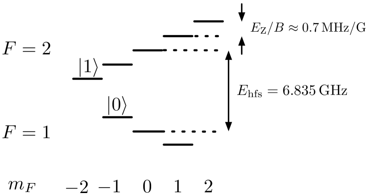
Figure 3: Energy diagram (not to scale) for the hyperfine split ground states of ⁸⁷Rb in the presence of an external Zeeman field. The states are labeled by total angular-momentum $F$ and $z$-projection $m_{F}$. Here, the qubit basis of the BEC is formed from the states $|F=1,m_{F}=-1\rangle$ and $|F=2,m_{F}=-2\rangle$. The total occupations of these two states differ by only a single atom.

In the following we show how to construct qubit states using two of the BEC’s internal atomic states, one of which is macroscopically populated. In second quantization the BEC Hamiltonian is modeled by

$$\hat{H}_{\rm B} =\sum_{\sigma=\uparrow,\downarrow}\int d{\bm{r}}\,\hat{\Psi}^{\dagger}_{\sigma}({\bm{r}})\left[-\frac{\nabla^{2}}{2m}+\omega_{\sigma}+V({\bm{r}})\right]\hat{\Psi}_{\sigma}({\bm{r}})$$

$$+\frac{1}{2}\sum_{\sigma,\sigma^{\prime}}{\sf g}_{\sigma,\sigma^{\prime}}\int d{\bm{r}}\,\hat{\Psi}^{\dagger}_{\sigma}({\bm{r}})\hat{\Psi}^{\dagger}_{\sigma^{\prime}}({\bm{r}})\hat{\Psi}_{\sigma^{\prime}}({\bm{r}})\hat{\Psi}_{\sigma}({\bm{r}}),$$ (38)

where $V({\bm{r}})$ is the center-of-mass trapping potential and $\omega_{\sigma}$ corresponds to the internal energy of each angular-momentum state. To form a qubit only two such angular-momentum states are needed. For definiteness and without loss of generality we take for these two states the ⁸⁷Rb states: $|\!\!\downarrow\rangle=|5^{2}S_{1/2},F=1,m_{F}=-1\rangle$ and $|\!\!\uparrow\rangle=|5^{2}S_{1/2},F=2,m_{F}=-2\rangle$, which from now on are labeled by a pseudospin index $\sigma=(\downarrow,\uparrow)$. These states, in the presence of a small Zeeman field, are separated in energy by $\omega_{\uparrow}-\omega_{\downarrow}\approx E_{\rm hfs}$, see Fig. 3. The interaction constants ${\sf g}_{\sigma,\sigma^{\prime}}$ correspond to the strengths of short-ranged pseudo-potentials used to model the complicated spin dependent atom-atom interactions and are, in the Born approximation, proportional to $s$-wave scattering lengths.

We now derive an approximation to the full Hamiltonian that captures the effects of coupling a flux qubit to an atomic BEC on the mean-field level. As we will see in the next section, the magnetic interaction between the BEC and SQUID only couples states in the BEC Hilbert space that differ by a single pseudospin. Thus, in the weak coupling limit, this leads us to conclude that the full Hilbert space of the BEC can be approximated by a two-dimensional subspace: the “ground state” with $N$ spin-$\downarrow$ and zero spin-$\uparrow$ atoms and an “excited state” with $N-1$ spin-$\downarrow$ and a single spin-$\uparrow$. This is analogous to the so-called rotating wave approximation, where the dominant process is the periodic transfer of a single quantum of energy from one subsystem to the other, i.e., the Rabi cycle.

At zero temperature the two many-body Fock states described above, differing by a single pseudospin, are the exact ground states of (III), which fully describe the condensate and non-condensed atoms, with slightly different densities. In principle, to proceed one would represent (III) in this two-dimensional basis. But as the exact grounds states are unknown, except possibly numerically for a small number of atoms, one has to perform a physically motivated approximation that captures the dominant effects. As the macroscopically occupied mode of the BEC makes the major contribution to any matrix element involved, we approximate the true ground states by Fock states with all the atoms in the BEC,

$$|0\rangle_{\rm B}= \frac{1}{\sqrt{N!}}\big{(}\hat{a}^{\dagger}_{\downarrow}\big{)}^{N}|{\rm vac}\rangle$$

$$|1\rangle_{\rm B}= \frac{1}{\sqrt{(N-1)!}}\big{(}\hat{a}^{\dagger}_{\downarrow}\big{)}^{N-1}\hat{a}^{\dagger}_{\uparrow}|{\rm vac}\rangle.$$ (39)

The above approximation of course neglects number fluctuations of the BEC and non-condensed atoms, but captures the leading order dependence on the condensate numbers of matrix elements of the Hamiltonian . The spatial wave function $\phi_{\sigma}({\bm{r}})$ of the single-particle state that corresponds to the creation and annihilation operators $a^{\dagger}_{\sigma}$ and $a_{\sigma}$ can be found within mean-field theory, i.e., from a Gross-Pitaevskiǐ  solution.

As the BEC Hamiltonian (III) conserves spin, its off-diagonal elements in the basis of (III) vanish, while the diagonal ones give the mean-field energies $E_{0,N},E_{1,N-1}$;

$$\hat{H}_{\rm B} \approx\left(\begin{array}[]{cc}E_{1,N-1}&0\\ 0&E_{0,N}\end{array}\right)$$ (42)

$$=\frac{E_{1,N-1}+E_{0,N}}{2}\openone+\frac{E_{1,N-1}-E_{0,N}}{2}\sigma_{z}.$$ (43)

Using that $E_{1,N-1}-E_{0,N}\simeq\omega_{\uparrow}-\omega_{\downarrow}\approx E_{\rm hfs}$, (the interaction renormalization of the hyperfine splitting being small compared to the level spacing) and omitting constant terms, the Hamiltonian (42) in the qubit basis, can finally be written in the simple form

$$\hat{H}_{\rm B}=\frac{E_{\rm hfs}}{2}\sigma_{z}.$$ (44)

IV BEC-SQUID Hybrid system

By coupling the BEC-SQUID together, a hybrid system can be formed. The coupling is done by using the electromagnetic field of the flux qubit to induce transitions between the spin states of the BEC and conversely atomic transitions in the BEC can energetically excite the flux states of the SQUID, see Fig. 4.

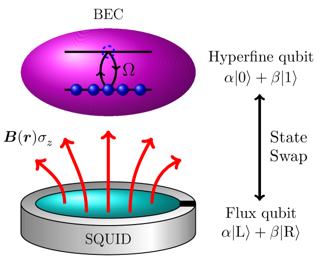
Figure 4: A schematic representation of a BEC-SQUID hybrid (not to scale). The flux qubit is created from energy eigenstates of the SQUID, formed by superposed left- and right-going currents, and coupled by its magnetic field to the hyperfine transition of an atomic BEC, where the Rabi process periodically flips one atom from a given hyperfine spin state to the other.

As the hyperfine states of the BEC considered here have the same spatial symmetry, which forbids electric dipole transitions, the transition is dominated by magnetic dipole coupling. The magnetic coupling of the BEC to the SQUID is given by the canonical expression

$$\hat{H}_{\rm int}=-\sum_{\sigma,\sigma^{\prime}}\int d{\bm{r}}\,\hat{\Psi}^{\dagger}_{\sigma}({\bm{r}})\big{[}{\bm{\mu}}\big{]}_{\sigma,\sigma^{\prime}}\hat{\Psi}_{\sigma^{\prime}}({\bm{r}})\otimes\hat{{\bm{B}}}({\bm{r}}),$$ (45)

multiplying the magnetic moment density of an atom with the local magnetic field and integrating over space. Here, $\bm{\mu}$ is the total magnetic moment matrix of atoms in the $\sigma$ basis. In the qubit basis of the BEC (III) and using Eq. (36) for the magnetic field operator of the SQUID

$$\hat{H}_{\rm int} \approx$$

$$-\left(\begin{array}[]{cc}(N-1){\bm{g}}_{\downarrow,\downarrow}\cdot\bm{\mu}_{\downarrow,\downarrow}+{\bm{g}}_{\uparrow,\uparrow}\cdot\bm{\mu}_{\uparrow,\uparrow}&\sqrt{N}{\bm{g}}_{\downarrow,\uparrow}\cdot\bm{\mu}_{\downarrow,\uparrow}\\ \sqrt{N}{\bm{g}}_{\uparrow,\downarrow}\cdot\bm{\mu}_{\uparrow,\downarrow}&N{\bm{g}}_{\downarrow,\downarrow}\cdot\bm{\mu}_{\downarrow,\downarrow}\end{array}\right)$$ (48)

$$\hskip 11.38092pt\otimes\sigma_{z},$$ (49)

where ${\bm{g}}_{\sigma,\sigma^{\prime}}=\int d{\bm{r}}\,\phi^{*}_{\sigma}({\bm{r}}){\bm{B}}({\bm{r}})\phi_{\sigma^{\prime}}({\bm{r}})$. The BEC provides a bosonic enhancement of the single-particle matrix elements, leading to the factors of $N$ and $\sqrt{N}$. Introducing a complex Rabi frequency $\Omega=\sqrt{N}{\bm{g}}_{\downarrow,\uparrow}\cdot\bm{\mu}_{\downarrow,\uparrow}$ Eq. (IV) can be written as

$$\hat{H}_{\rm int} =-\frac{(2N-1){\bm{g}}_{\downarrow,\downarrow}\cdot\bm{\mu}_{\downarrow,\downarrow}+{\bm{g}}_{\uparrow,\uparrow}\cdot\bm{\mu}_{\uparrow,\uparrow}}{2}\openone\otimes\sigma_{z}$$

$$-\frac{{\bm{g}}_{\uparrow,\uparrow}\cdot\bm{\mu}_{\uparrow,\uparrow}-{\bm{g}}_{\downarrow,\downarrow}\cdot\bm{\mu}_{\downarrow,\downarrow}}{2}\sigma_{z}\otimes\sigma_{z}-\left(\begin{array}[]{cc}0&\Omega\\ \Omega^{*}&0\end{array}\right)\otimes\sigma_{z}.$$ (52)

The first term of (IV) simply leads to a renormalization of the SQUID states and can be absorbed by a rescaling of the flux qubit parameters, while the $\sigma_{z}\otimes\sigma_{z}$ interaction is much smaller than the last term and can be neglected in comparison. Thus, the qubit-qubit coupling term is taken to be

$$\hat{H}_{\rm int}\approx-\left(\begin{array}[]{cc}0&\Omega\\ \Omega^{*}&0\end{array}\right)\otimes\sigma_{z}.$$ (53)

An estimate for the Rabi frequency can be obtained by calculating the magnetic field of the SQUID from (II.3) using a SQUID radius of $d=1\,\mu{\rm m}$ that is carrying a current of $I=1$  mA. The BEC spatial wave functions $\phi_{\sigma}({\bm{r}})$ can be roughly approximated by the ground state of a 3-D harmonic oscillator, with a trapping frequency of $\omega_{\rm ho}=2\pi\times 50$  Hz. Then, for a condensate with $N=10^{6}$ atoms and a center-to-center BEC-SQUID separation of $50\,\mu{\rm m}$, $|\Omega|\approx 0.1$ MHz. A larger coupling can be achieved by moving the BEC closer to the SQUID. For example, for a BEC-SQUID separation of only $10\,\mu{\rm m}$ leads to $|\Omega|\approx 10$ MHz. There are, however, potential detrimental effects caused by having the BEC in too close proximity to a (comparatively hot) surface, such as increased heating or spin flips caused by thermal emission from the SQUID Cano ; Kasch .

Finally, putting together the Hamiltonians of the flux qubit (21), the hyperfine qubit (44), and coupling (53), the total Hamiltonian of the hybrid system is

$$\hat{H}=\hat{H}_{\rm B}\oplus\hat{H}_{\rm S}+\hat{H}_{\rm int},$$ (54)

where the direct sum is defined by $\hat{A}\oplus\hat{B}=\hat{A}\otimes\openone+\openone\otimes\hat{B}$. Next, we show how to manipulate quantum information within this hybrid architecture.

V State transfer & BEC-SQUID entanglement

Here, we show that one can transfer arbitrary qubit states initially prepared in the SQUID to the BEC, with high fidelity. This is done by dynamically manipulating the energy level spacing of the flux qubit, bringing the two subsystems into and out of resonance for half a Rabi period. Although the energy level spacing of flux qubits have been experimentally tuned on sub-nanosecond time scales Paauw ; Castellano , to remain in the low-energy qubit subspace of the SQUID, the level modulation should be quasi-adiabatic. This requires the inverse of the time scale of the dynamics to be much smaller than the energy needed to leave the flux qubit subspace, which is typically on the order of several GHz. To model this, we allow the tunneling parameter appearing in the flux qubit Hamiltonian (21) to become time dependent, i.e., $\Delta\to\Delta(t)$. Furthermore, for simplicity we assume the left and right current states are degenerate, i.e., setting $\varepsilon=0$ in (21). In the energy eigenstate basis the flux qubit Hamiltonian is then

$$\hat{H}_{\rm S}=\frac{\Delta(t)}{2}\sigma_{z},$$ (55)

with corresponding energy eigenstates

$$|0\rangle_{\rm S} =\frac{1}{\sqrt{2}}\big{(}|{\rm L}\rangle+|{\rm R}\rangle)$$

$$|1\rangle_{\rm S} =\frac{1}{\sqrt{2}}\big{(}|{\rm L}\rangle-|{\rm R}\rangle).$$ (56)

Along with the hyperfine qubit basis (III), the computational basis is taken to be $|ij\rangle=|i\rangle_{\rm B}\otimes|j\rangle_{\rm S}$. The total Hamiltonian (54) in this basis is then

$$\hat{H}(t)=\frac{E_{\rm hfs}}{2}\sigma_{z}\oplus\frac{\Delta(t)}{2}\sigma_{z}-\left(\begin{array}[]{cc}0&\Omega\\ \Omega^{*}&0\end{array}\right)\otimes\sigma_{x}.$$ (59)

To transfer an arbitrary qubit state that is first prepared in the flux qubit to the BEC, the general time-dependence of $\Delta(t)$ should be as follows: Initially the two subsystems should be out of resonance, $E_{\rm hfs}\neq\Delta(t)$; then, over a short time period, the ramp time, the two systems are brought into resonance, $E_{\rm hfs}=\Delta(t)$, for half a Rabi period $T_{\rm R/2}=\pi/(2|\Omega|)$; finally, the two qubits are brought out of resonance again, leaving the initial flux qubit state in the hyperfine qubit with some final fidelity. Specifically we set $\Delta(t)=E_{\rm hfs}W(t)$, where $W(t)$ is a unitless function of time, that is composed of hyperbolic tangents that smoothly ramp the system into and out of resonance Window function . The ramping time is defined as the time over which the level spacing changes from being 1% greater than its off resonance value, chosen to be $E_{\rm hfs}/2$, to within 1% of being on resonance.

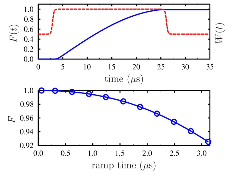
Figure 5: The top panel shows the time-dependent fidelity of the direct transfer $|01\rangle\to|10\rangle$ from the flux qubit to the BEC states. The dashed line shows the profile of the function $W(t)$ used to bring the two systems into and out of resonance for half a Rabi period, with a ramping time of approximately 1 $\mu\rm s$ Window function . The bottom panel shows the final fidelity of the transfer as a function of ramp times.

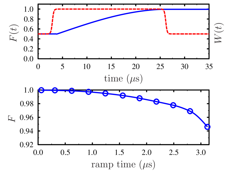
Figure 6: The top panel shows the time-dependent fidelity of the transfer of the superposition state $2^{-1/2}\big{(}|00\rangle+i|01\rangle\big{)}\to 2^{-1/2}\big{(}|00\rangle+i|10\rangle\big{)}$. As in Fig. 5, the dashed line shows the profile of the function $W(t)$ used to bring the two systems into and out of resonance, with a ramping time of approximately 1 $\mu\rm s$ Window function . The bottom panel shows the final fidelity of the transfer as a function of ramp times.

The fidelity of the transfer is defined as $F(t)=|\langle\Psi_{\rm target}|\Psi(t)\rangle|$, where $|\Psi(t)\rangle$ is the time evolved initial state, and $|\Psi_{\rm target}\rangle$ is the sought-after final state. The time evolution of $|\Psi(t)\rangle$ is numerically determined using the time-dependent Hamiltonian (59). Figure 5 shows the fidelity during the transfer of the state $|\Psi\rangle=|01\rangle$ and the dependence of the final fidelity on the ramping time. Figure 6 shows the same for the superposition state $|\Psi\rangle=2^{-1/2}\big{(}|00\rangle+i|01\rangle\big{)}$. As can be seen from Figs. 5 and 6 high fidelities, greater than 99%, can be achieved, even for relatively long ramping times, and, for a given ramping time, the final transfer fidelity is weakly state dependent. The state can be transferred back to the SQUID by again bringing the two system into and out of resonance. Therefore, with the exceptionally long coherence times of the hyperfine states, this system is an ideal prospective candidate for long-term storage of quantum information.

Additionally, instead of transferring a state from one subsystem to the other, one can entangle the BEC and SQUID. This is done by first preparing the system in $|\Psi\rangle=|01\rangle$ and then bringing the two qubits into and out of resonance for only a quarter of a Rabi period. This will produce the maximally entangled state $|\Psi\rangle=2^{-1/2}\big{(}|01\rangle+|10\rangle\big{)}$, see Fig. 7. For such states, quantum correlations between the two subsystems can be probed, for example, by Bell’s inequalities. In the next section we describe how to experimentally determine the hyperfine qubit state, which is needed to test such relations, using single-atom spectroscopy.

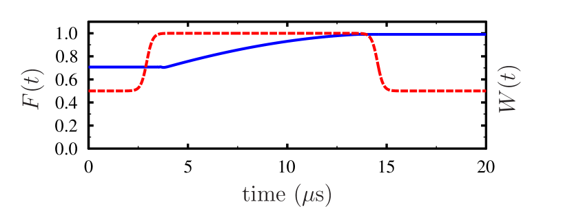
Figure 7: Here the fidelity of producing the maximally entangled qubit-qubit state $|\Psi\rangle=2^{-1/2}\big{(}|01\rangle+|10\rangle\big{)}$ is shown. This is done by first preparing the system in the state $|01\rangle$ and then bringing the two subsystems into resonance for only a quarter of a Rabi period. The ramp time used, approximately 1 $\mu\rm s$, is the same as in Figs. 5 and 6.

VI Tomography of the BEC qubit

Measuring the state of the hyperfine qubit has to be delicately handled. In principle one could independently measure the density of each pseudospin. The existence of a nonzero spin-$\uparrow$ density would indicate the $|1\rangle_{\rm B}$ state. But this relies on determination of densities on the single atom level, a possible but quite demanding task, that also destroys the trapped BEC. Instead we propose a nondestructive scheme using spectroscopy to determine the occupation of the spin-$\uparrow$ hyperfine state. By measuring the absorption of an external radiation source tuned to the transition energy of the spin-$\uparrow$ state and an unoccupied level, one effectively performs a single measurement of the hyperfine pseudospin $\hat{S}_{z}=\frac{1}{2}\sigma_{z}$ operator, see Fig. 8. Such a measurement would collapse the BEC qubit onto either the $|0\rangle_{\rm B}$ or $|1\rangle_{\rm B}$ state and could be used to probe entangled states of the BEC-SQUID system.

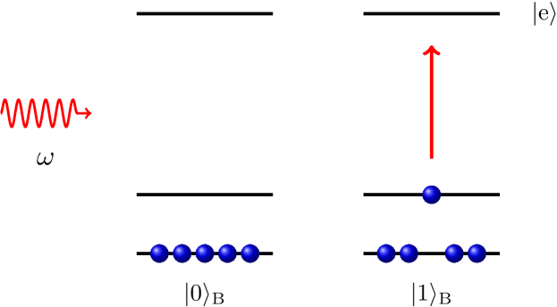
Figure 8: To measure the $\hat{S}_{z}$ operator component of the BEC pseudospin, an external laser source can be used to probe the occupation of the upper hyperfine state. If there is no absorption for light tuned to the transition between the upper hyperfine state and some experimentally convenient higher excited state $|{\rm e}\rangle$, e.g. another empty hyperfine level, then this would correspond to the system being in the $|0\rangle_{\rm B}$, or spin-$\downarrow$, state. On the other hand, if absorption occurs, this would correspond to the $|1\rangle_{\rm B}$ qubit state.

To fully characterize the state of the BEC qubit requires reconstructing its density matrix from measurements of a complete set of observables, so-called quantum tomography QCbook . A general density matrix of a pseudospin-$\frac{1}{2}$ system can be written as

$$\rho=\frac{1}{2}\big{(}\openone+{\bm{a}}\cdot\bm{\sigma}\big{)},$$ (60)

where ${\bm{a}}\in\mathbb{R}$ such that $\|\bm{a}\|=1$, and $\bm{\sigma}=(\sigma_{x},\sigma_{y},\sigma_{z})$. Using the facts that ${\rm Tr}\,\sigma_{i}=0$ and ${\rm Tr}\,\sigma_{i}\sigma_{j}=2\delta_{i,j}$ one can show

$$\langle\hat{S}_{x}\rangle={\rm Tr}\,\rho\hat{S}_{x} =a_{x}/2$$ (61a)

$$\langle\hat{S}_{y}\rangle={\rm Tr}\,\rho\hat{S}_{y} =a_{y}/2$$ (61b)

$$\langle\hat{S}_{z}\rangle={\rm Tr}\,\rho\hat{S}_{z} =a_{z}/2,$$ (61c)

where $\hat{S}_{i}=\frac{1}{2}\sigma_{i}$ are the spin operators. Thus, by experimentally measuring the expectation values for each spin direction the density matrix can be reconstructed.

As described above, the expectation value of $\hat{S}_{z}$ can be found by averaging repeated measurements of identically prepared states of the BEC qubit, i.e., states prepared in the flux qubit, passed to the BEC, and then measured. As only $\hat{S}_{z}$ is directly measurable a modified protocol must be used to determine the expectation value of $\hat{S}_{x}$ and $\hat{S}_{y}$. To obtain the expectation value of $\hat{S}_{x}$ and $\hat{S}_{y}$ for a given state or density matrix $\rho$ one can measure $\hat{S}_{z}$ of a rotated state $\rho^{\prime}$. To see this one notes that $S_{z}$ is related to $S_{x}$ and $S_{y}$ by a unitary transformation;

$$\hat{S}_{x} =e^{-i\frac{\pi}{2}\hat{S}_{y}}\hat{S}_{z}e^{i\frac{\pi}{2}\hat{S}_{y}}$$ (62a)

$$\hat{S}_{y} =e^{i\frac{\pi}{2}\hat{S}_{x}}\hat{S}_{z}e^{-i\frac{\pi}{2}\hat{S}_{x}}.$$ (62b)

Thus to obtain $\langle\hat{S}_{x}\rangle$ with respect to $\rho$

$$\langle\hat{S}_{x}\rangle ={\rm Tr}\,\rho e^{-i\frac{\pi}{2}\hat{S}_{y}}\hat{S}_{z}e^{i\frac{\pi}{2}\hat{S}_{y}}={\rm Tr}\,e^{i\frac{\pi}{2}\hat{S}_{y}}\rho e^{-i\frac{\pi}{2}\hat{S}_{y}}\hat{S}_{z}$$

$$={\rm Tr}\,\rho^{\prime}\hat{S}_{z},$$ (63)

where $\rho^{\prime}=e^{i\frac{\pi}{2}\hat{S}_{y}}\rho e^{-i\frac{\pi}{2}\hat{S}_{y}}$. Hence, one prepares and measures $\hat{S}_{z}$ for the rotated state $\rho^{\prime}$ to obtain $\langle\hat{S}_{x}\rangle$ for the desired state $\rho$ and similarly for $\langle\hat{S}_{y}\rangle$. Using these values to reconstruct the desired density matrix, the fidelity of the state transfer can be experimentally determined.

VII Conclusion

We have proposed a novel hybrid quantum system, which could be an ideal candidate for long-term storage of qubit states, comprised of the hyperfine states of an atomic BEC magnetically coupled to a flux qubit. The potential of almost infinite coherence times of the hyperfine qubit is advantageous and highly desirable, while the qubit-qubit coupling, and thus the transfer time, can be tuned by adjusting the BEC-SQUID separation. Furthermore, we propose a straightforward method of using atomic spectroscopy to experimentally determine the hyperfine qubit density matrix, which would enable the determination of the state transfer fidelity or quantum correlations of entangled BEC-SQUID systems.

Additional open questions that are left for future work concern the effects of interactions and beyond mean-field effects, as well as finite temperature on the BEC state, both of which lead to decoherence and depletion of the condensate state. These are potentially difficult effects to capture accurately, as the simple two-dimensional qubit Hilbert space has to be enlarged to infinite dimensions.

- (1) Z-L. Xiang, S. Ashhab, J. Q. You, and F. Nori, Rev. Mod. Phys. 85, 623 (2013).
- (2) M. Aspelmeyer, T. Kippenberg, and F. Marquardt, arXiv: 1303.0733.
- (3) A. D. O’Connell et al., Nature 464, 697 (2010).
- (4) A. Blais, R-S. Huang, A. Wallraff, S. M. Girvin, and R. J. Schoelkopf, Phys. Rev. A 69, 062320 (2004).
- (5) J. Verdú, H. Zoubi, Ch. Koller, J. Majer, H. Ritsch, and J. Schmiedmayer, Phys. Rev. Lett. 103, 043603 (2009).
- (6) M. D. Lukin, Rev. Mod. Phys. 75, 457 (2003).
- (7) A. D. Armour, M. P. Blencowe, and K. C. Schwab, Phys. Rev. Lett. 88, 148301 (2002).
- (8) Y. Nakamura, Yu. A. Pashkin, and J. S. Tsai, Nature 398, 786 (1999).
- (9) A. Wallraff et al., Nature 431, 162 (2004).
- (10) X. Zhu et al., Nature 478, 221 (2011).
- (11) H. Wu et al., Phys. Rev. Lett. 105, 140503 (2010).
- (12) J. Majer et al., Nature 449, 443 (2007).
- (13) A. N. Cleland and M. R. Geller, Phys. Rev. Lett. 93, 070501 (2004).
- (14) P. Rabl et al., Phys. Rev. Lett. 97 033003 (2006).
- (15) F. Brennecke et al., Nature 450, 268 (2007).
- (16) K. Baumann, C. Guerlin, F. Brennecke, and T. Esslinger, Nature 464, 1301 (2010).
- (17) M. Blencowe, Nature 468, 44 (2010).
- (18) T. van der Sar et al., Nature 484, 82 (2012).
- (19) S. Bernon et al., eprint arXiv:1302.6610.
- (20) K. R. Patton and U. R. Fischer, EPL 102, 20001 (2013).
- (21) J. Clarke and A. I. Braginski, The SQUID Handbook: Fundamentals and Technology of SQUIDs and SQUID Systems, (Wiley-VCH, Weinheim, 2004).
- (22) V. Ambegaokar, U. Eckern, and G. Schön, Phys. Rev. Lett. 48, 1745 (1982).
- (23) J. D. Jackson, Classical Electrodynamics, (John Wiley & Sons, New York, 1998).
- (24) S. Stringari, C. E. Wieman, and M. Inguscio Bose-Einstein Condensation in Atomic Gases (Proceedings of the International School of Physics), (IOS Press, Amsterdam, 1999).
- (25) D. Cano et al., Eur. Phys. J. D 63, 17 (2011).
- (26) R. Fermani, T. Müller, B. Zhang, M. J. Lim, and R. Dumke, J. Phys. B: At. Mol. Opt. Phys. 43, 095002 (2010).
- (27) F. G. Paauw, A. Fedorov, C. J. P. M. Harmans, and J. E. Mooij, Phys. Rev. Lett. 102, 090501 (2009).
- (28) M. G. Castellano, F. Chiarello, P. Carelli, C. Cosmelli, F. Mattioli, and G. Torrioli, New J. Phys. 12, 043047 (2010).
- (29) Explicitly, , where , is the time the two systems are on resonance (typically for a half or a quarter of a Rabi cycle), and is the off-resonance value of the SQUID tunneling amplitude, , in units of (we set for all our calculations). The function is a smoothed step function, such that ; different ramp times are obtained by varying .
- (30) M. A. Nielsen and I. L. Chuang, Quantum Computation and Quantum Information, (Cambridge University Press, Cambridge, England, 2000).