An X-Ray Study of Supernova Remnant N49 and Soft Gamma-Ray Repeater 0526–66 in the Large Magellanic Cloud

Abstract

We report on the results from our deep Chandra observation (120 ks) of the supernova remnant (SNR) N49 and soft $\gamma$-ray repeater (SGR) 0526–66 in the Large Magellanic Cloud. We firmly establish the detection of an ejecta “bullet” beyond the southwestern boundary of N49. The X-ray spectrum of the bullet is distinguished from that of the main SNR shell, showing significantly enhanced Si and S abundances. We also detect an ejecta feature in the eastern shell, which shows metal overabundances similar to those of the bullet. If N49 was produced by a core-collapse explosion of a massive star, the detected Si-rich ejecta may represent explosive O-burning or incomplete Si-burning products from deep interior of the supernova. On the other hand, the observed Si/S abundance ratio in the ejecta may favor Type Ia origin for N49. We refine the Sedov age of N49, $\tau_{\rm Sed}~{}\sim$ 4800 yr, with the explosion energy $E_{0}~{}\sim$ 1.8 $\times$ 10⁵¹ erg. Our blackbody (BB) + power law (PL) model for the quiescent X-ray emission from SGR 0526–66 indicates that the PL photon index ($\Gamma~{}\sim$ 2.5) is identical to that of PSR 1E1048.1–5937, the well-known candidate transition object between anomalous X-ray pulsars and SGRs. Alternatively, the two-component BB model implies X-ray emission from a small ($R~{}\sim$ 1 km) hot spot(s) ($kT~{}\sim$ 1 keV) in addition to emission from the neutron star’s cooler surface ($R~{}\sim$ 10 km, $kT~{}\sim$ 0.4 keV). There is a considerable discrepancy in the estimated column toward 0526–66 between BB+PL and BB+BB model fits. Discriminating these spectral models would be crucial to test the long-debated physical association between N49 and 0526–66.

1 INTRODUCTION

The supernova remnant (SNR) N49 is the third brightest X-ray SNR in the Large Magellanic Cloud (LMC). The blast wave is interacting with dense clumpy interstellar clouds on the SNR’s eastern side (Vancura et al., 1992; Banas et al., 1997), producing bright emission in optical, infrared, ultraviolet, and X-ray bands (Park et al. 2003a, ; Sankrit et al., 2004; Williams et al., 2006; Rakowski et al., 2007; Bilikova et al., 2007; Otsuka et al., 2010), which revealed the shock structures in N49 down to sub-pc scales over wide ranges of the velocity ($v$ $\sim$ 10^2-3 km s^-1), temperature ($T$ $\sim$ 10^2-7 K), and the interacting density ($n$ $\sim$ 1–10³ cm^-3). The blast wave in the western side of the SNR appears to be propagating into a lower density medium than in the east (Dickel & Milne, 1998). Early studies estimated overall low metal abundances in N49, indicating that metal-rich ejecta might have been substantially intermixed with the interstellar medium (ISM) of the LMC (Danziger & Leibowitz, 1985; Russell & Dopita, 1990; Hughes et al., 1998).

The origin of N49 has been elusive (thermonuclear vs. core-collapse explosion). The interstellar environment of N49, indicated by the presence of nearby molecular clouds (Banas et al., 1997) and young stellar clusters (Klose et al., 2004) and its location within an OB association (Chu & Kennicutt, 1988) generally support a core-collapse origin for N49 from a massive progenitor star. One model suggested that N49 is interacting with a dense shell of a Strömgren sphere created by a massive B-type progenitor (Shull et al., 1985). The positional coincidence of a soft $\gamma$-ray repeater (SGR) 0526–66 within the boundary of N49 (Cline et al., 1982; Rothschild et al., 1994) may also suggest a core-collapse origin from a massive star, if this SGR is the compact remnant of the SN that created N49. However, the physical association between SNR N49 and SGR 0526–66 is uncertain (Gaensler et al., 2001; Klose et al., 2004; Badenes et al., 2009). Based on the ASCA data, Hughes et al. (1998) found no evidence for surrounding ISM that had been modified by stellar winds from the massive progenitor.

Nucleosynthesis studies of metal-rich ejecta in SNRs using spatially-resolved X-ray spectroscopy are useful to constrain the progenitor’s mass (e.g., Hughes et al., 2003; Park et al. 2003b, ; Park et al., 2004, 2007). Although bright X-ray features in N49 are apparently dominated by emission from the shock-cloud interaction, previous Chandra observations have shown marginal evidence for enhanced emission lines and overabundant metal elements from a few sub-regions in the SNR (Park et al. 2003a, ). For instance, a promising ejecta candidate was a small protrusion beyond the SNR’s southwestern boundary. This emission feature was suggested to be a candidate ejecta bullet, but metal overabundances were not conclusive because of poor photon statistics (Park et al. 2003a, ). Also, because N49 was detected significantly off-axis (by $\sim$6$.\mkern-4.0mu^{\prime}$5) in the previous Chandra data (ObsID 1041) used by Park et al. (2003a), the point spread function (PSF) was substantially distorted, and the true morphology of this feature (point-like vs. extended) was uncertain. We note that there were three other on-axis Chandra observations of N49(Kulkarni et al., 2003). These previous observations were not useful to study the ejecta bullet candidate because of either the use of a CCD subarray or a very short exposure. Thus, a firm detection of metal-rich ejecta in N49 remains elusive.

Here we report on initial results from our new Chandra observation of N49. Our new Chandra data present $\sim$4 times deeper exposure (for the entire N49) than the data used by Park et al. (2003a), with an on-axis pointing to N49. With these new data, we clearly detect some metal-rich ejecta features in N49. Combining the new data with archival data, we also perform a detailed spectral analysis of SGR 0526–66. In this paper, we report on the results from our spectral analysis of SGR 0526–66 and the detected metal-rich ejecta features in N49. Our studies of complex shock-cloud interaction regions of N49 and the timing analysis of SGR 0526–66 will be presented in a subsequent paper. We describe the observations and the data reduction in Section 2. The image and spectral analyses are presented in Section 3, and a discussion in Section 4. A summary will be presented in Section 5.

2 OBSERVATIONS & DATA REDUCTION

We observed N49 with the Advanced CCD Imaging Spectrometer (ACIS) on board Chandra X-Ray Observatory on 2009 July 18 – September 19 (ObsIDs 10123, 10806, 10807, and 10808) during AO10. We chose the ACIS-S3 chip to utilize the best sensitivity and energy resolution of the detector in the soft X-ray band. The pointing ($\alpha$₂₀₀₀ = 05^h 25^m 58^s.8, $\delta$₂₀₀₀ = $-$66^∘ 05^′ 00$.\mkern-4.0mu^{\prime\prime}$0) was roughly toward the geometrical center of N49. SGR 0526–66 and the ejecta bullet candidate are detected within $\sim$30^′′ and $\sim$40^′′ of the aim point, respectively. We used a 1/4 subarray of the ACIS-S3 to ensure low photon pileup ($\mathrel{\hbox{\hbox to0.0pt{\hbox{\lower 4.0pt\hbox{$\sim$}}\hss}\hbox{$<$}}}$ 5%) of SGR 0526–66, and to allow us to detect the 8 s pulsations from the SGR, while still obtaining full coverage of the entire SNR N49. We processed the raw event files following the standard data reduction methods using CIAO 4.2 and Chandra CALDB 4.3.0, which includes correction for the charge transfer inefficiency (CTI). We applied the standard data screening by status and grade (ASCA grades 02346). We performed this data reduction on individual observations. The overall light curve from the entire S3 chip for each ObsID showed no evidence of flaring particle background. Then, we merged four data sets into a single event file by re-projecting them onto ObsID 10807’s tangential plane. After the data reduction, the total effective exposure is $\sim$108 ks.

We also used two data sets (ObsIDs 747 and 1957) available in the Chandra archive. The pointing of these archival data was toward the position of SGR 0526–66 ($\alpha$₂₀₀₀ = 05^h 26^m 00^s.7, $\delta$₂₀₀₀ = $-$66^∘ 04^′ 35$.\mkern-4.0mu^{\prime\prime}$0), and thus they provide a high resolution imaging of N49 as well as the SGR. Although these archival data cannot be used to study south-southwestern regions (including the ejecta bullet candidate) of N49 due to the use of 1/8 subarray of the ACIS-S3, they covered east-northeastern parts of the SNR with a decent exposure (a total of $\sim$88 ks by combining ObsIDs 747 and 1957). Thus, these data are useful to study eastern regions of N49 and SGR 0526–66. We re-processed these two archival data sets in the same way as we did for our new observation data. Combining all these observations, our data present the deepest coverage with the high resolution X-ray imaging spectroscopy for SNR N49 ($\sim$108 ks in the south-west regions and $\sim$196 ks in the north-east regions) and SGR 0526–66 ($\sim$196 ks). Our new Chandra observations and archival data used in this work are summarized in Table 1.

3 ANALYSIS & RESULTS

3.1 X-ray Images

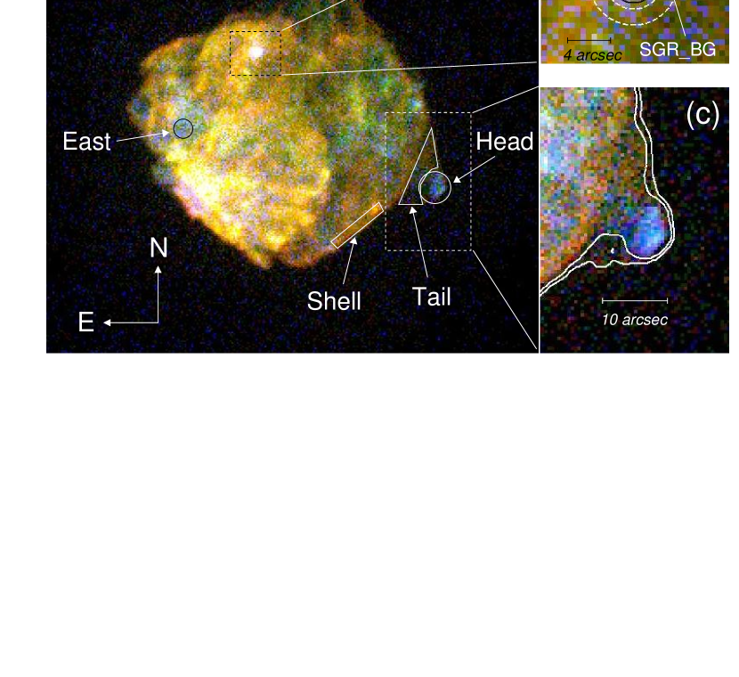
Figure 1: (a) A 3-color ACIS images of N49 based on our 2009 data. Regions used for our spectral analysis are marked. (b) A zoom-in image of the SGR 0526–66 region. The source and background regions used for the spectral analysis of SGR 0526–66 are shown. (c) A zoom-in of the southwestern region of N49 including the ejecta bullet. Contours for the outer boundary of N49 are overlaid. In (a), (b), and (c), Color codes are: red is 0.3–0.8 keV, green is 0.8–1.7 keV, and blue is 1.7–7.0 keV band. The pixel size is 0$.\mkern-4.0mu^{\prime\prime}$5 in all panels.

An X-ray color image of N49 shows complex asymmetric X-ray emission features (Figure 1a). These features have been partially revealed by previous Chandra data (Park et al. 2003a, ; Kulkarni et al., 2003). Our new deep Chandra image reveals all those fine X-ray structures throughout the entire SNR with substantially improved photon statistics and resolution (Figure 1a). The outer boundary of N49 appears as a thin shell radiating in soft X-rays (reddish in Figure 1a) that represents the blast wave sweeping through the general ambient medium of the LMC. A notable exception is the candidate ejecta bullet extending beyond the SNR shell in the southwest, which is distinctively blue in color (Figure 1c). Bright X-ray filaments in the eastern parts of the SNR are regions where the shock is interacting with dense clumpy clouds (Park et al. 2003a, , and references therein). These shock-cloud interaction regions show a wide range in X-ray colors at angular scales down to several arcseconds. The western parts of N49 are relatively faint and X-ray emission is emphasized in green to blue while showing some red filamentary features as well (Figure 1a). This general color variation across the SNR appears to be related to the temperature variation caused by the overall interstellar density distribution, in which dense clouds are interacting with the shock mostly in the eastern half of the SNR (e.g., Park et al. 2003a, ).

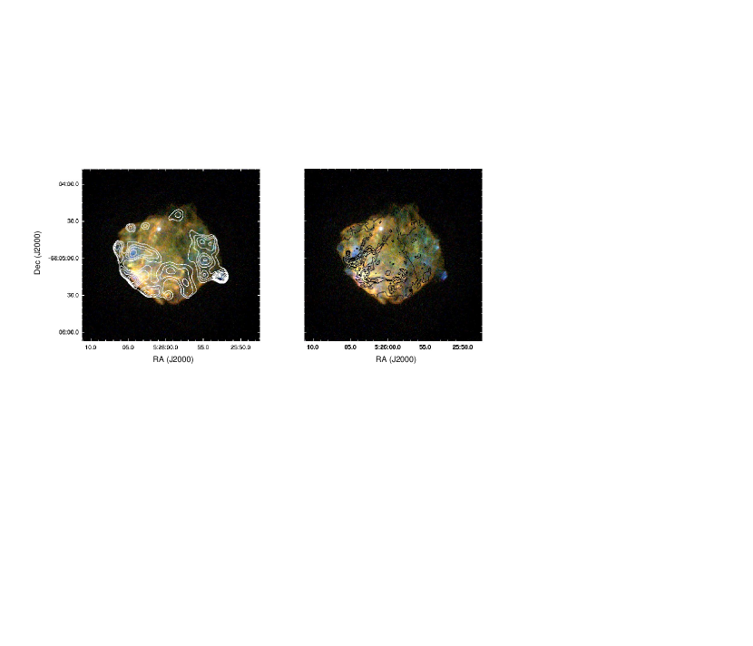
Figure 2: (a) An X-ray 3-color image of N49 with contours of Si EW map overlaid. Color codes are the same as those in Figure 1. The Si He$\alpha$ + Ly$\alpha$ ($E$ = 1.75 – 2.1 keV) EW has been calculated by the methods described in Park et al. (2003a). (b) The same X-ray color image as in (a), overlaid with contours of an archival Hubble Space Telescope image.

The spectrally-hard, blue protrusion extending beyond the main SNR shell in the southwestern boundary was proposed to be a candidate ejecta bullet based on the previous low-resolution Chandra data (Park et al. 2003a, ). If it is indeed an ejecta bullet, this feature is reminiscent of “shrapnel” found in the Vela SNR (Aschenbach et al., 1995), but nearly two orders of magnitude more distant. Our new Chandra data clearly resolve this feature. It is an extended feature with a head ($\sim$4^′′ in radius) and a tail that connects the head to the main SNR shell (the “Head” and “Tail” regions in Figure 1a, respectively). The blue color of the Head region is likely due to enhanced line emission in the hard X-ray band: e.g., the Si (He$\alpha$ + Ly$\alpha$) line equivalent width (EW) map shows a strong enhancement in the Head region (Figure 2a), which suggests a metal-rich ejecta for the origin of this feature. In fact, our spectral analysis of the Head region shows highly overabundant Si and S (see Section 3.2.2). The Tail region appears to be composed of a central hard (blue) emission region surrounded by a soft (red), conical region (Figure 1c). It is likely the turbulent region behind the bullet, in which the metal-rich ejecta and shocked ISM are intermixed, possibly enclosed by the sides of a bow-shock produced by the bullet’s supersonic motion. The bow shock, however, is not prominent ahead of the bullet, possibly due to unfavorable viewing geometry. The axis bisecting the opening angle ($\sim$87^∘) is roughly pointing back to the geometric center of the SNR, but not exactly toward SGR 0526–66.

We noticed that there is a small region in the eastern part of the SNR (the “East” region in Figure 1a), which shows similar characteristics to those of the Head region: i.e., this region stands out with a distinctively blue color in the bright eastern half of the SNR, and it is coincident with a strongly enhanced Si line EW (Figure 2a). The East region corresponds to an inter-cloud region (Figure 2b) in which a possibility of metal overabundance was suggested by our previous work (Park et al. 2003a, ). Our spectral analysis of this region indeed reveals its metal-rich ejecta nature (see Section 3.2.2).

3.2 X-ray Spectra

Based on results from our image analysis, we extracted spectra from several regions that appear to characteristically represent distinctive features: i.e., the swept-up interstellar medium (the “Shell” and “SGR_BG” regions), shocked metal-rich ejecta (the “Head” and “East” regions), and the connecting region between the ejecta bullet and the main SNR shell (the “Tail” region). These regions are marked in Figures 1a & 1b. We also extracted the spectrum from the quiescent X-ray counterpart of SGR 0526–66 (the “SGR” region in Figure 1b). We present the spectral analysis of these swept-up medium, ejecta features, and 0526–66 in Sections 3.2.1, 3.2.2, and 3.2.3, respectively.

3.2.1 N49: Swept-Up Interstellar Medium

The brightest X-ray emission in the eastern parts of N49 originates from the shock interaction with clumpy clouds with a density gradient spanning a few orders of magnitudes (Vancura et al., 1992). X-ray emission from such a clumpy medium would represent a complex mixture of gas temperatures and ionization states. Such a plasma condition is likely localized in strong shock-cloud interaction regions. While the western regions do not show evidence of shock interaction with dense clumpy clouds, they also show some significant X-ray color variation (Figure 1a). For those regions, it is not straightforward to characterize the X-ray emission spectrum of the general ambient medium shocked by the blast wave. Thus, to study the nature of the general swept-up ISM and the SNR’s overall dynamics, we extracted the X-ray spectrum from a region in the outermost rim of the SNR in the southern boundary (the “Shell” region in Figure 1a) in which no complex spectral and/or spatial substructures are seen. We also used a small annular region surrounding SGR 0526–66 (the “SGR_BG” region in Figure 1b) to characterize background emission for SGR 0526–66. Since the SGR_BG region is in the transition area between the bright eastern and faint western parts of the SNR, it may also effectively show an average plasma condition of the complex shock structures across the SNR.

For our spectral analysis, we re-binned the observed spectra to contain a minimum of 20 counts per energy channel. We fit the X-ray spectrum with a non-equilibrium ionization (NEI) state plane-shock model (vpshock model in conjunction with the NEI version 2.0 in the XSPEC software, Borkowski et al., 2001) that is based on ATOMDB (Smith et al., 2001). We used an augmented version of this atomic database to include inner-shell processes (e.g., lines from Li-like ions) and updates of the Fe L-shell lines, whose effects are substantial in under-ionized plasma, but are not incorporated in the standard XSPEC NEI version 2.0. We fixed the Galactic column at $N_{\rm H,Gal}$ = 6 $\times$ 10²⁰ cm^-2 toward N49 (Dickey & Lockman, 1990). We fit the foreground column by the LMC ($N_{\rm H,LMC}$) assuming the LMC abundances available in the literature (He = 0.89, C = 0.30, N = 0.12, O = 0.26, Ne = 0.33, Na = 0.30, Mg = 0.32, Al = 0.30, Si = 0.30, S = 0.31, Cl = 0.31, Ar = 0.54, Ca = 0.34, Cr = 0.61, Fe = 0.36, Co = 0.30, and Ni = 0.62, Russell & Dopita, 1992; Hughes et al., 1998). Hereafter, elemental abundances are with respect to Solar (Anders & Grevesse, 1989).

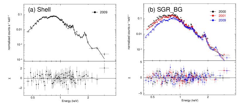
Figure 3: (a) X-ray spectrum of “Shell” region. (b) X-ray spectrum of “SGR_BG” region. In (a) and (b), the best-fit plane-shock model is overlaid. The lower panel is the residuals from the best-fit model.

The southern boundary of N49 was not covered by ObsIDs 747 and 1957 because of the use of a 1/8 subarray. Thus, we used our new Chandra data to extract the spectrum from the Shell region. The background was subtracted using the spectrum extracted from two circular source-free regions (with a radius of 8^′′) beyond the south-western boundary of the SNR. The Shell region spectrum contains significant photon statistics of $\sim$4600 counts, and can be well fitted by the NEI plane-shock model ($\chi^{2}$/n = 49.1/68 with the electron temperature $kT$ = 0.57 keV and the ionization timescale $n_{e}t$ = 6.35 $\times$ 10¹¹ cm^-3 s, Figure 3a). The foreground column by the LMC is estimated to be $N_{\rm H,LMC}$ $\sim$ 0.9 $\times$ 10²¹ cm^-2. The best-fit metal abundances are generally consistent with the LMC values. Results from this spectral model fit are summarized in Tables 2 & 3.

The SGR_BG region was observed by ObsIDs 747 and 1957 as well as our new Chandra observations, and thus, we used all of those data to extract the spectrum from this region. The total photon statistics for this region is $\sim$13600 counts. The background was subtracted using the spectrum extracted from a circular source-free region (with a radius of 8^′′) beyond the northern boundary of the SNR. We initially fit these three data sets simultaneously with all fitted parameters tied with each other. Although the overall fit may be acceptable ($\chi^{2}$/n = 1.28), there appears to be a small systematic offset in the normalization at $E$ $\mathrel{\hbox{\hbox to0.0pt{\hbox{\lower 4.0pt\hbox{$\sim$}}\hss}\hbox{$<$}}}$ 1 keV between data taken in 2000/2001 (ObsIDs 747 and 1957) and in 2009 (ObsIDs 10123+10806+10807+10808). Considering the fact that the time separation between 2000/2001 and 2009 observations is substantial and that the effect appears to be emphasized in the soft band ($E$ $\mathrel{\hbox{\hbox to0.0pt{\hbox{\lower 4.0pt\hbox{$\sim$}}\hss}\hbox{$<$}}}$ 1 keV), this small discrepancy is likely related to the calibration effect by the time-dependent quantum efficiency degradation in the ACIS. Since the quantum efficiency degradation affects the spectral modeling as if there is an “extra” foreground absorption, we attempted the model fit with $N_{\rm H,LMC}$ untied among three spectra. The best-fit $N_{\rm H,LMC}$ values are the same between 2000 and 2001 data, while it is $\sim$25% larger for the 2009 data. Thus, we repeated the spectral model fit with $N_{\rm H,LMC}$ tied only between 2000 and 2001 data, and with that for 2009 data allowed to vary freely. The fit improved somewhat ($\chi^{2}$/n = 1.19). The best-fit columns are $N_{\rm H,LMC}$ = 1.39${}^{+0.46}_{-0.47}$ $\times$ 10²¹ cm^-2 and 1.76${}^{+0.43}_{-0.38}$ $\times$ 10²¹ cm^-2 for the 2000/2001 and 2009 data, respectively. While showing a marginal calibration effect, these values are consistent within statistical uncertainties (hereafter, errors are with a 90% confidence level). In the following discussion, we assume the average value of $N_{\rm H,LMC}$ = 1.58${}^{+0.45}_{-0.44}$ $\times$ 10²¹ cm^-2. The best-fit spectral parameters for the SGR_BG region are $kT$ $\sim$ 0.56 keV and $n_{e}t$ $\sim$ 9.65 $\times$ 10¹¹ cm^-3 s, all of which are consistent with those for the Shell region within uncertainties. The best-fit metal abundances are also generally consistent with those from the Shell region. These model parameters are summarized in Tables 2 & 3.

3.2.2 N49: Metal-Rich Ejecta

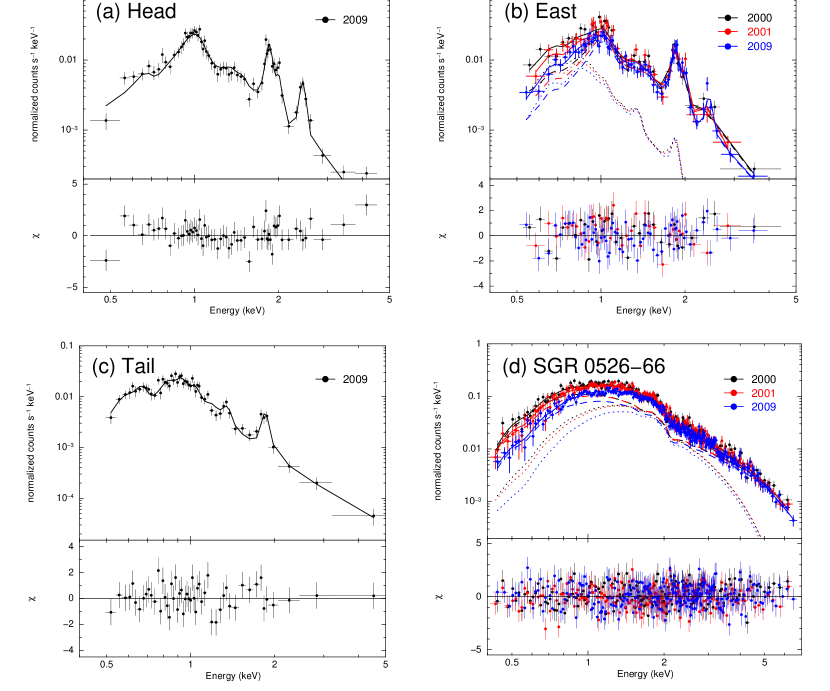
Figure 4: X-ray spectrum of (a) “Head”, (b) “East”, (c) “Tail”, and (d) SGR 0526–66. In (a), (b), and (c), the best-fit plane-shock model is overlaid (solid curve). In (d), the best-fit BB+PL model is overlaid (solid curve). In (b), dashed and dotted curves show model components for the ejecta and the superposed emission from the shocked cloud, respectively. In (d), dashed and dotted curves show the best-fit PL and BB model components, respectively. The lower panel is the residuals from the best-fit model.

Our new Chandra data clearly resolve the extended nature of the ejecta fragment bullet (the Head region) and the trailing tail-like hot gas (the Tail region, Figure 1c). Because the bullet region was not covered by the 2000/2001 data, we used only 2009 data for the spectral analysis of this feature. We extracted $\sim$1800 counts from the Head region. In contrast to those for the swept-up medium, the X-ray spectrum of the Head region shows remarkably enhanced emission lines from highly ionized Si and S (Figure 4a), which is consistent with the corresponding bright Si line EW image (Figure 2a). We fitted this spectrum with an NEI plane-shock model following the method described in Section 3.2.1. The background was subtracted using the same spectrum as we used for the Shell region. We initially fixed metal abundances at the best-fit values for the Shell region (Table 3), which resulted in a statistically unacceptable fit ($\chi^{2}$/n = 3.3) primarily because of the strongly enhanced Si and S lines. Varying Si and S abundances provides an acceptable fit ($\chi^{2}$/n = 67.0/59, Figure 4a). The best-fit LMC column ($N_{\rm H,LMC}$ $\sim$ 1.3 $\times$ 10²¹ cm^-2) is consistent with those estimated from the Shell and SGR_BG regions. The electron temperature ($kT$ $\sim$ 1 keV) and the ionization timescale ($n_{e}t$ $>$ 2 $\times$ 10¹² cm^-3 s) are significantly higher than those from swept-up medium. The Si ($\sim$2.3) and S ($\sim$3.2) abundances are an order of magnitude larger than the LMC values, firmly establishing the metal-rich ejecta nature of the bullet.

Varying other elemental abundances (O, Ne, Mg, and Fe) somewhat improves the fit ($\chi^{2}$/n = 49.3/55, but the corresponding F-probability is marginal [$\sim$0.002]), and the best-fit electron temperature is very high ($kT$ $\sim$ 4 keV). In addition to the overabundant Si and S, the best-fit abundance appears to be moderately enhanced for O ($\sim$0.7), Ne ($\sim$2.1), and Mg ($\sim$1.0). However, these abundances are not well constrained (with a factor of $\mathrel{\hbox{\hbox to0.0pt{\hbox{\lower 4.0pt\hbox{$\sim$}}\hss}\hbox{$>$}}}$2 uncertainties), and thus the overabundance for these elements is not convincing based on the current data. We conclude that the main differences in the fitted parameters resulting from varying metal abundances other than Si and S (i.e., the high $kT$ $\sim$ 4 keV and possibly enhanced abundances for O, Ne, and Mg) are not compelling. Otherwise, it does not affect our discussion of the ejecta features (see Section 4.1). Thus, we hereafter discuss the nature of the bullet based on our spectral model fit with only Si and S abundances varied. The results from the Head region model fit are summarized in Tables 2 & 3.

The Tail region is faint, and we extracted $\sim$1500 counts in this region. We fit this spectrum with an NEI plane shock model $\chi^{2}$/n = 44.9/44, Figure 4c). The Tail region is fitted by the X-ray spectrum from a hot gas ($kT$ $\sim$ 2 keV) in a significantly under-ionized state ($n_{e}t$ $\sim$ 7 $\times$ 10¹⁰ cm^-3 s). The best-fit elemental abundances are consistent with those estimated from the Shell and SGR_BG regions. We note that the Tail region shows substructures of the spectrally-hard (blue) interior surrounded by soft (red) outer layer (Figure 1c). It suggests that the Tail region may be a mixture of metal-rich ejecta and shocked swept-up medium. Thus, we attempted an alternative spectral model, assuming two shock components, a soft component for the swept-up ISM and a hard component for the metal-rich ejecta. The spectral parameters, except for the normalization, and metal abundances for the ejecta component were fixed at the best-fit values estimated from the Head region. The metal abundances for the soft component were fixed at the values estimated from the Shell region. The electron temperature, ionization timescale, and the normalization parameters for the soft component were varied freely. The observed Tail spectrum can be equally fitted by this two-component model ($\chi^{2}$/n = 52.4/49). In this model fit, the metal-rich ejecta component contributes $\sim$15% of the total observed X-ray flux in the 0.5–10 keV band. These one- and two-component models are not statistically distinguished with the current data. Results from these Tail region spectral model fits are summarized in Tables 2 & 3.

The East region shows a distinctively blue color (Figure 1a) with a strong enhancement in the Si line EW image (Figure 2a), which resembles the spectral properties of the Head region of the bullet. This region corresponds to a hot inter-cloud region (Park et al. 2003a, ). This region may also be a candidate ejecta feature, probably isolated from the complex emission from shocked dense clumpy clouds (Figure 2b). Since this region was covered by both the 2000/2001 and 2009 data, we used all of these data to extract the X-ray spectrum. We extracted the X-ray spectrum from a small circular region with a radius of 2^′′, in which the Chandra data allowed us total photon statistics of $\sim$3600 counts. The background was subtracted using the spectrum extracted from two circular source-free regions (with a radius of 8^′′) beyond the eastern boundary of the SNR. We fit the observed spectrum with the NEI plane shock model. Because enhanced Si-K and S-K lines are evident, we varied Si and S abundances while fixing other abundances at average values estimated from the Shell and SGR_BG regions. The fitted parameters are $N_{\rm H,LMC}$ $\sim$ 0.8 $\times$ 10²¹ cm^-2, $kT$ $\sim$ 1.05 keV, and $n_{e}t$ $>$ 52.4 $\times$ 10¹¹ cm^-3 s. The estimated Si and S abundances are high (Si $\sim$ 1.8 and S $\sim$ 1.4). While the fit may be acceptable ($\chi^{2}$/n = 173.4/134), there appear to be some systematic residuals at $E$ $\mathrel{\hbox{\hbox to0.0pt{\hbox{\lower 4.0pt\hbox{$\sim$}}\hss}\hbox{$<$}}}$ 1 keV. Based on the results from our spectral analysis of the ejecta (the Head region) and the swept-up ISM (the Shell and SGR_BG regions) regions, we consider that the East region emission is a superposition of the spectrally-hard metal-rich ejecta and the projected soft swept-up ISM components. To account for the contribution of soft X-ray emission from the shocked ISM in the observed spectrum of the East region, we added an NEI model component for which we fixed the electron temperature, ionization timescale, and metal abundances at the average values estimated from the Shell and SGR_BG regions. Only the normalization parameter was varied for this component. This model fit significantly improves ($\chi^{2}$/n = 144.4/133) without affecting the best-fit parameters for the hard, ejecta component. The only noticeable change is a larger value for the best-fit $N_{\rm H,LMC}$ $\sim$ 3 $\times$ 10²¹ cm^-2. This larger estimate for $N_{\rm H,LMC}$ appears to be consistent with the presence of dense molecular clouds toward eastern parts of the SNR. The assumed soft component from the swept-up ISM contributes $\sim$20% of the total observed X-ray flux in the 0.5–5 keV band. The results from this fit are summarized in Table 2 & 3.

3.2.3 SGR 0526–66

The X-ray spectrum of SGR 0526–66 is extracted from a circular region of 2^′′ radius (Figure 1b). The background spectrum is characterized by emission from an annular region (2^′′ in thickness) around the source (the SGR_BG region, Figure 1b) to average the complex diffuse emission from SNR N49 projected against the SGR. Since archival Chandra data (ObsIDs 747 and 1957) were pointed at the SGR with a decent exposure (Table 1), we used these archival data as well as our new data for the spectral analysis of SGR 0526–66. We fit these three spectra simultaneously. Just like our spectral analysis of N49, we assumed that the SGR spectrum is absorbed by both Galactic (fixed at $N_{\rm H,Gal}$ = 6 $\times$ 10²⁰ cm^-2) and LMC columns ($N_{\rm H,LMC}$).

Initially, we fit the SGR spectrum with a single power law (PL) in which we tied all fitted parameters between the three sets of the spectrum. The best-fit model from this fit is not acceptable ($\chi$²/$n$ $\sim$ 1.8). The best-fit model shows significant residuals at $E$ $\mathrel{\hbox{\hbox to0.0pt{\hbox{\lower 4.0pt\hbox{$\sim$}}\hss}\hbox{$>$}}}$ 0.8 keV, because it underestimates the overall flux level for the 2000/2001 data while it overestimates the flux level for the 2009 data. Thus, we untied the normalization parameter between the 2000/2001 and 2009 data, and then repeated the model fit. The fit improved ($\chi$²/$n$ $\sim$ 1.5) with a $\sim$15% lower normalization for the 2009 data than that for the 2000/2001 data. Although statistically improved by removing the normalization offset between the 2000/2001 and 2009 data, we do not accept this fit because systematic residuals are evident over the entire bandpass with a relatively high $\chi$²/$n$ $\sim$ 1.5. Alternatively, we attempted a single blackbody (BB) model fit. The best-fit models are statistically unacceptable ($\chi$²/$n$ $\sim$ 2.2 and 2.5 with the untied and tied normalization parameter between the 2000/2001 and 2009 data, respectively).

Kulkarni et al. (2003) showed that a PL+BB model was needed to adequately describe the quiescent X-ray emission from SGR 0526–66. On the other hand, Park et al. (2003a) argued that there could have been a considerable contamination from the surrounding soft thermal X-ray emission in the SGR spectrum presented by Kulkarni et al. (2003), and that the need for a BB component was not conclusive. Our SGR spectrum with $\sim$4 times higher photon statistics than that used by Park et al. (2003a) indicates that a PL model cannot describe the observed SGR spectrum, supporting the conclusion by Kulkarni et al. (2003). Thus, we fit the SGR spectrum with a PL+BB model. We repeated the general steps as we did with a single PL model fits: i.e., we first tied all fitted parameters between the 2000/2001 and 2009 data sets, and then untied them one at a time (i.e., BB temperature [$kT_{\rm BB}$], PL photon index [$\Gamma$], and normalizations for the BB and PL components). The best-fit values for $kT_{\rm BB}$ and $\Gamma$ are consistent within uncertainties between the 2000/2001 and 2009 data. The normalization for the BB and/or PL components are fitted to be $\sim$10–30% lower for the 2009 data than they are for the 2000/2001 data. The fit improvement due to this normalization change is statistically significant, and the fit is acceptable ($\chi$²/$n$ = 577.4/582). The normalization change appears to be more effective for the PL component than for the BB, probably because the PL component covers a broader range of the observed spectrum than the BB component (The PL component contributes $\sim$70% of the total observed flux in the 0.5–10 keV band).

While the X-ray spectra of SGRs and anomalous X-ray pulsars (AXPs) are usually fitted with a BB+PL model (e.g., Mereghetti, 2007), double BB models (BB+BB) have also been suggested to fit some AXPs (e.g., Halpern & Gotthelf, 2005). A recent work showed that a BB+BB model fit can successfully reproduce the observed Chandra spectrum (taken in 2000 and 2001) of SGR 0526–66 (Nakagawa et al., 2009). Thus, we attempted to fit our SGR spectrum with a BB+BB model. We tied BB temperatures between 2000/2001 and 2009 data since we found no evidence of change in the temperatures. Just like our BB+PL modeling, we varied normalizations freely between 2000/2001 and 2009. The fit is statistically good ($\chi$²/$n$ = 616.4/582). Although statistical uncertainties are relatively large, a $\sim$15% decrease in the best-fit value of the normalization parameters are suggested for both BB components, which is similar to the results from the BB+PL model fit.

Both of the BB+PL and BB+BB model fits suggest that the overall X-ray flux of SGR 0526–66 in the 0.5–10 keV band has been reduced by $\sim$15% in 2009 compared with that in 2000/2001. We note that we used a 1/4 subarray of the ACIS-S3 in our 2009 observations, while a 1/8 subarray was used in 2000 and 2001. Based on the event grade distribution, we found that the photon pileup effect is similarly small in both data sets ($\sim$2% in 2000 and 2001 vs. $\sim$4% in 2009). Nonetheless, assuming the X-ray flux observed in 2000/2001, we estimated the pileup effect on the X-ray flux measurements in 2009 data using the Portable Interactive Multi-Mission Simulator (PIMMS). Our PIMMS simulations predict that the pileup effect in 2009 data would reduce the 0.5–10 keV band X-ray flux in 2009 by $\mathrel{\hbox{\hbox to0.0pt{\hbox{\lower 4.0pt\hbox{$\sim$}}\hss}\hbox{$<$}}}$5% compared with that measured in 2000/2001. We also tested the pileup effect by applying an ACIS pileup model (Davis, 2001) for our spectral model fits. This model indicated that the 0.5–10 keV flux estimates with the 2009 data are probably affected by $\mathrel{\hbox{\hbox to0.0pt{\hbox{\lower 4.0pt\hbox{$\sim$}}\hss}\hbox{$<$}}}$5% due to the use of 1/4-subarray. Thus, although the flux change between 2000/2001 and 2009 is partially caused by pileup effect, the pileup is not responsible for the entire flux change. The apparent flux change is unlikely due to uncertainties in the detector calibration for the time-dependent quantum efficiency degradation, because there is no evidence for discrepancy in the fitted normalization parameters that is emphasized in the soft band ($E$ $\mathrel{\hbox{\hbox to0.0pt{\hbox{\lower 4.0pt\hbox{$\sim$}}\hss}\hbox{$<$}}}$ 1 keV) between 2000/2001 and 2009 data. Thus, while follow-up Chandra observations are required to draw a firm conclusion on the nature of the long-term X-ray light curve of 0526–66, we tentatively conclude that the discrepancy in the observed X-ray flux of SGR 0526–66 between 2000/2001 and 2009 is probably real rather than an artifact due to the photon pile-up and/or an inaccurate calibration of the time-dependent quantum efficiency degradation between two epochs. The SGR spectrum and the best-fit BB+PL model are presented in Figure 4d. Results from the best-fit BB+PL and BB+BB model fits are summarized in Table 4 and 5, respectively.

4 DISCUSSION

4.1 N49

Based on the volume emission measure ($EM$) estimated from the spectral fit of the Shell region, we calculate the post-shock electron density ($n_{e}$) behind the blast wave. We assumed an emission volume of $V$ $\sim$ 9.4 $\times$ 10⁵⁵ cm³ for a 3^′′ $\times$ 18^′′ region (corresponding to $\sim$0.7 pc $\times$ 4.4 pc, hereafter we assume $d$ = 50 kpc for the LMC) with a $\sim$1 pc path-length along the line of sight. We also assumed $n_{e}$ = 1.2 $n_{H}$ for a mean charge state with normal composition. The best-fit $EM$ (= 6.75 $\times$ 10⁵⁷ cm^-3) implies $n_{e}$ $\sim$ 9.3$f^{-{1\over 2}}$ cm^-3 and $n_{H}$ $\sim$ 7.7$f^{-{1\over 2}}$ cm^-3, where $f$ is the volume filling factor of the X-ray emitting gas. The pre-shock H density is then $n_{0}$ $\sim$ 1.9$f^{-{1\over 2}}$ cm^-3 for a strong adiabatic shock where $n_{H}$ = 4$n_{0}$. Assuming an adiabatic shock in electron-ion temperature equipartition, the gas temperature is related with the shock velocity ($v$) as $T$ = 3$\bar{m}$$v^{2}$/16$k$ where $k$ is the Boltzmann constant and $\bar{m}$ $\sim$ 0.6 $m_{p}$ is the mean molecular weight with the proton mass $m_{p}$ = 1.67 $\times$ 10^-24 g. For the gas temperature of $kT$ = 0.57 keV, the shock velocity $v$ $\sim$ 700 km s^-1 is estimated. Thus, for the radius of $\sim$8.5 pc (assuming the angular distance of $\sim$35^′′ between the Shell region and the geometric center of N49), we estimate the Sedov age of the SNR, $\tau_{\rm Sed}$ $\sim$ 4800 yr. The estimated $\tau_{\rm Sed}$ and $n_{0}$ imply an explosion energy of $E_{0}$ $\sim$ 1.8$f^{-{1\over 2}}$ $\times$ 10⁵¹ erg. The estimated Sedov age is $\sim$30% lower than our previous estimate ($\sim$6600 yr, Park et al. 2003a, ) for which we assumed $n_{0}$ = 0.9 cm^-3 based on optical data (Vancura et al., 1992) and the canonical value of the SN explosion energy ($E_{0}$ = 1 $\times$ 10⁵¹ erg). Also, the previous estimate was based on a more complex spectral modeling of multi-temperature plasma in the eastern regions of the SNR for which an accurate estimate of the distance from the SNR center was not feasible. Thus, we conclude that our new estimate of the SNR age is more reliable, while being in plausible agreement with the previous estimate by Park et al. (2003a).

The presence of the ejecta bullet beyond the southwestern shell of N49 is conclusively established by our new Chandra observation. The on-axis ACIS image clearly resolves the bullet into a head and a tail extending back to the main shell of the SNR. The head region itself is an extended feature ($\sim$4^′′ in radius) with an enhanced intensity toward the inferred direction of motion (Figure 1c). The X-ray color of the head is distinctively blue in contrast to reddish color of the overall SNR shell. The foreground column ($N_{\rm H,LMC}$ $\sim$ 1.3 $\times$ 10²¹ cm^-2) toward the head is consistent with those to N49’s main shell and the bullet’s tail region, which supports that the blue color is intrinsic for the head rather than being caused by a significantly larger foreground absorption (in which case the head would probably be a background source). In fact, the observed X-ray spectrum (Figure 4a) shows that the hardness of the head is due to highly enhanced line emission from He- and H-like Si and He-like S ions. The estimated abundances for Si ($\sim$2.3) and S ($\sim$3.2) are an order of magnitude larger than the LMC values. We note that Park et al. (2003a) suggested a possibility of the enhanced abundance for O in addition to Si and S in the bullet. However, the overabundance for O is not confirmed by our new data. Nonetheless, the highly overabundant Si and S firmly establish the identification of the bullet as metal-rich stellar fragment ejected from the deep interior of the progenitor star.

The East region shows nearly identical spectral characteristics to the Head region: i.e., a distinctively blue color compared with surrounding regions and strongly enhanced Si and S lines. Just like the Head region, significantly enhanced Si and S abundances are estimated, but overabundances for other metal species are not required to describe the observed spectrum. The foreground absorption for the East region appears to be larger than other regions of N49, and it is probably caused by nearby dense molecular clouds which are interacting with the SNR in the eastern regions (e.g., Banas et al., 1997; Otsuka et al., 2010). If the excess column ($\Delta$$N_{\rm H,LMC}$ $\sim$ 2 $\times$ 10²¹ cm^-2 compared with the average $N_{\rm H,LMC}$ $\sim$ 1.2 $\times$ 10²¹ cm^-2 estimated for other regions of N49, Table 2) originates from these nearby molecular clouds, the corresponding average cloud density of $n_{H}$ $\sim$ 90 cm^-3 is implied for the overall cloud size of $R$ $\sim$7 pc (the size estimated by Banas et al. 1997). This average density is in plausible agreement with the pre-shock density range of the clumpy clouds ($n_{0}$ $\sim$ 20–940 cm^-3, Vancura et al. 1992) with which N49 is interacting, while it is significantly larger than the value we estimated for the Shell region ($n_{0}$ $\sim$ 1.9 cm^-3) where the shock is propagating into the low density ambient medium.

Based on the Si and S abundances and volume emission measures of these metal-rich ejecta features, we estimate the Si to S ejecta mass ratio. The observed spectrum of the Head and East regions shows that He- and H-like ionization states dominate for Si, while S ions are primarily in He-like state. Thus, for simplicity, we assumed a “pure” ejecta case with electron to ion density ratios of $n_{e,{\rm Si}}$ $\approx$ 12.5 $n_{\rm Si}$ and $n_{e,{\rm S}}$ $\approx$ 14 $n_{\rm S}$. For dominant isotopes of ²⁸Si and ³²S, the measured Si and S abundances imply the ejecta mass ratio $M_{\rm Si}$/$M_{\rm S}$ $\sim$ 1.2 and 1.6 ($V_{\rm Si}$/$V_{\rm S}$)${}^{1\over 2}$, where $V_{\rm Si}$ and $V_{\rm S}$ are the volume of Si- and S-rich hot ejecta gas, respectively. Assuming $V_{\rm Si}$ $\approx$ $V_{\rm S}$, the estimated mass ratios are $M_{\rm Si}$/$M_{\rm S}$ $\sim$1.2 for the Head region and $\sim$1.6 for the East region. The mixture of H in metal-rich ejecta may not significantly affect our mass ratio estimates as long as the ISM mixture rate is similar between the Si and S ejecta. We compare these $M_{\rm Si}$/$M_{\rm S}$ with standard SN nucleosynthesis models. Our estimated $M_{\rm Si}$/$M_{\rm S}$ appears to be smaller than those for core-collapse SN models in which $M_{\rm Si}$/$M_{\rm S}$ typically ranges $\sim$2–4 depending on the progenitor’s mass (e.g., Nomoto et al. 1997a, ; Rauscher et al., 2002; Limongi & Chieffi, 2003). The Si to S mass ratio for Type Ia SN models ($M_{\rm Si}$/$M_{\rm S}$ $\sim$ 1.5 – 1.8, e.g., Nomoto et al. [1997b]; Iwamoto et al. [1999]) are generally smaller than core-collapse cases, which are closer to our estimates for N49. The lack of evidence for O-rich ejecta in the Head and East regions is generally suggestive of a Type Ia origin as well. If we take $\sim$0.3 (Table 3) as an upper limit for the O abundance of the SN nucleosynthesis in N49, $M_{\rm O}$/$M_{\rm Si}$ $<$ 1.4 can be inferred for the Head region. This limit appears to be consistent with Type Ia models ($M_{\rm O}$/$M_{\rm Si}$ $\mathrel{\hbox{\hbox to0.0pt{\hbox{\lower 4.0pt\hbox{$\sim$}}\hss}\hbox{$<$}}}$ 1, e.g., Nomoto et al. [1997b]; Iwamoto et al. [1999]), while being smaller than those for core-collapse models ($M_{\rm O}$/$M_{\rm Si}$ $>$ 2, e.g., Nomoto et al. [1997a]; Limongi & Chieffi [2003]).

On the other hand, the Head and East regions do not show evidence for overabundant Fe, which is usually considered as an iconic feature for Type Ia SNRs. The lack of Fe-rich ejecta is problematic for a Type Ia interpretation, and it would rather support a core-collapse origin. Also, the suggested Type Ia origin for N49 is inconsistent with its interstellar environment with recent star-forming regions and nearby molecular clouds, which rather suggests a massive progenitor for N49 (e.g., Chu & Kennicutt, 1988; Banas et al., 1997; Klose et al., 2004; Badenes et al., 2009). If N49 is a remnant of a core-collapse explosion from a massive progenitor rather than a Type Ia, the Si-rich nature of the Head and East regions may be generally considered to be explosive O-burning or incomplete Si-burning products from deep inside of the core-collapse SN. In fact, Si-rich ejecta knots have been detected in core-collapse SNRs: e.g., Shrapnel A in Vela SNR (Miyata et al., 2001) and those found in Cassiopeia A (Hughes et al., 2000).

While the possibility of Type Ia origin for N49 is intriguing, we caution that the utility of our $M_{\rm Si}$/$M_{\rm S}$ estimate to identify the SN type is limited, because it is based on small localized ejecta features whereas SN nucleosynthesis model calculations are for the integrated ejecta material from the entire SN. Thus, based on the current data, our discussion on the origin of N49 is far from conclusive. A more extensive ejecta search and comprehensive nucleosynthesis study are required to reveal the true origin of N49. We point out that the correct identification of N49’s origin is particularly important because of its astrophysical implications in the context of the SNR’s environment. For instance, if N49 is the remnant of a Type Ia SN, the long-standing argument for its physical association with SGR 0526–66 is unambiguously ruled out. A Type Ia origin for N49 may also suggest an intriguing case for a prompt population Ia SN from a relatively young white dwarf progenitor in analogy to the scenario suggested for SNR 0104–72.3 in the Small Magellanic Cloud (Lee et al., 2011).

4.2 SGR 0526–66

Our deep Chandra observation firmly establishes the previously suggested two-component X-ray spectrum for SGR 0526–66. The PL index ($\Gamma$ $\sim$ 2.5) of its X-ray spectrum is intermediate between those for other SGRs ($\Gamma$ $\sim$ 1–2) and AXPs ($\Gamma$ $\sim$ 3–4), which suggests that SGR 0526–66 may be a transition object between the SGR and AXP states (Kulkarni et al., 2003). In fact, our estimated PL index ($\Gamma$ $\sim$ 2.5) is identical to that of AXP 1E 1048.1–5937, which is considered to be a clear case of a SGR-AXP transition object (Gavriil et al., 2002). The implied size of the BB radiation ($R_{\rm BB}$ $\sim$ 5–6 km) is smaller than the canonical size of neutron stars. The small $R_{\rm BB}$ suggests the existence of restricted hot spots on the surface of the neutron star.

Alternatively, a BB+BB model can equally describe the observed spectrum of 0526–66. The two-component BB model was preferred for some AXPs, because the second BB component is physically more reasonable than the steep PL component to explain the low flux limit at longer wavelengths (e.g., Halpern & Gotthelf, 2005). Recently, Nakagawa et al. (2009) showed that the X-ray spectrum of the quiescent emission from 0526–66 can be fitted by a two-component BB model. Our result is consistent with that by Nakagawa et al. (2009). The hard BB component indicates a small emission area ($R$ $\sim$ 1 km) with a hot temperature of $kT$ $\sim$ 1 keV. The soft BB component indicates an area corresponding to the entire surface of the neutron star ($R$ $\sim$ 10 km) with a lower temperature of $kT$ $\sim$ 0.4 keV. These overall characteristics are reminiscent of the peculiar types of neutron stars found at the center of several young SNRs (e.g., Pavlov et al., 2000; Park et al., 2009), but the estimated BB temperatures of 0526–66 are significantly higher than those estimated in others.

The overall X-ray flux in the 0.5–10 keV band in 2009 is $\sim$15% lower than it was in 2000–2001. We show a long-term X-ray light curve of SGR 0526–66 in Figure 5. In Figure 5, we plot the mean flux of 2000 and 2001 data (the middle data point) because the observed flux is indistinguishable between the two epochs. We added the fluxes estimated by the ROSAT HRI data in this light curve. For the ROSAT fluxes, we converted the observed HRI count rate (1.51$\pm$0.13 $\times$ 10^-2 counts s^-1, Rothschild et al., 1994) into the 0.5–10 keV band energy flux using PIMMS. In this calculation, we assumed two cases of BB+PL and BB+BB models with the best-fit parameters listed in Tables 4 and 5, respectively. We also assumed the fractional contributions in the observed 0.1–2.4 keV band HRI count rate from each of the model components, based on the results summarized in Table 4 and 5. The calculated ROSAT HRI fluxes are $f_{\rm 0.5-10~{}keV}$ $\sim$ 1.34 (BB+PL) and $\sim$1.17 (BB+BB) $\times$ 10^-12 erg cm^-2 s^-1. While the X-ray flux appears to have decreased by $\sim$30% since 1992 based on the BB+PL case, the overall flux decrease is less certain for the BB+BB case. If it is real, the suggested X-ray flux change for 0526–66 would not be surprising, because long-term variabilities by a factor of up to $\sim$10 in several years have been detected in some AXPs (e.g., Baykal et al., 1996; Oosterbroek et al., 1998). Follow-up Chandra observations are essential to reveal the true nature of the long-term light curve of SGR 0526–66.

We note that the foreground column to 0526–66 shows a significant discrepancy by a factor of $\sim$3 between values estimated by two different spectral modelings (BB+PL vs. BB+BB). The column estimated by the BB+BB model fit ($N_{\rm H,LMC}$ $\sim$ 1.7 $\times$ 10²¹ cm^-2) is generally in agreement with those measured for N49 (Table 2), and particularly, it is fully consistent with the column toward the SGR_BG region ($N_{\rm H,LMC}$ $\sim$ 1.6 $\times$ 10²¹ cm^-2). These consistent columns between N49 and 0526–66 are supportive of the long-suggested physical association between them. On the other hand, our BB+PL model fit of 0526–66 spectrum shows a substantially larger foreground column for SGR 0526–66 ($N_{\rm H,LMC}$ $\sim$ 5.4 $\times$ 10²¹ cm^-2) than that for SGR_BG region. If this is the case, the large difference in the foreground absorption between SNR N49 and SGR 0526–66 brings into question their physical association. If we assumed an average interstellar density of $n_{0}$ $\sim$ 1–2 cm^-3 (see Section 4.1) near N49, SGR 0526–66 may be $\sim$500–1000 pc beyond N49. Thus, this model-dependent difference in $N_{\rm H,LMC}$ for 0526–66 deserves full attention for further studies with follow-up observations. An H I survey of the LMC shows that N49 and 0526–66 are projected toward the dense boundary between two supergiant shells (Kim et al., 2003). The estimated H I column density toward this region appears to be $N_{\rm H,LMC}$ $\sim$ 5 $\times$ 10²¹ cm^-2. It is difficult to discriminate our model-dependent $N_{\rm H,LMC}$ measurements toward 0526–66 based on this relatively large column estimated by H I data with a poor angular resolution ($\sim$1^′ which is comparable with the angular size of N49). We note that, if 0526–66 and N49 are associated, the projected angular separation ($\sim$22^′′) of 0526–66 from the geometric center of N49 requires a large kick-velocity (i.e., an average transverse velocity of $v$ $\sim$ 1100 km s^-1 for the SNR age of $\sim$4800 yr). At least, the proper measurement of the foreground column toward 0526–66 is directly related with two important astrophysical issues: (1) the origin of the quiescent X-ray emission from SGR 0526–66, and (2) the physical relationship between SNR N49 and SGR 0526–66. It may also provide a useful piece of puzzle to reveal the origin of SNR N49 (thermonuclear vs. core-collapse).

5 SUMMARY

Using our deep Chandra observation, we detect metal-rich ejecta features in SNR N49. These ejecta features include a “bullet” that is most likely a stellar fragment travelling beyond the southwestern boundary of the SNR. We also find an ejecta feature in the eastern part of the SNR, nearly in the opposite side of the SNR to the bullet. Both of these ejecta features show highly enhanced Si and S abundances by an order of magnitude above the LMC values. We do not find compelling evidence for overabundant O and/or Fe in these ejecta features. If N49 is a remnant of a core-collapse explosion of a massive progenitor, the Si-rich nature of ejecta may be considered to be nucleosynthesis products of explosive O-burning or incomplete Si-burning from deep inside of the SN. On the other hand, the estimated Si- and S-rich ejecta mass ratio appears to favor a Type Ia origin for N49. If N49 was the remnant of a Type Ia SN, the suggested physical association between N49 and SGR 0526–66 would be unambiguously ruled out. However, we note that our SN ejecta study is limited because we used only some small localized ejecta features rather than the integrated ejecta composition from the entire SNR to represent the true SN nucleosynthesis. Follow-up studies to reveal the comprehensive ejecta composition in N49 are required to unveil the true origin of this SNR.

Our new Chandra observation allows us to detect the blast wave forming the swept-up shell in the southern boundary with significant photon statistics. Since this part of the shell is not affected by spectral complications due to the SNR’s interaction with dense clumpy clouds, it provides a useful opportunity to reveal the dynamics of the SNR more accurately than previous works. We estimate the Sedov age of $\tau_{\rm Sed}$ $\sim$ 4800 yr and the explosion energy $E_{0}$ $\sim$ 1.8 $\times$ 10⁵¹ erg for N49.

Our spectral analysis of the quiescent X-ray emission from SGR 0526–66 using the deep exposure clearly reveals the presence of a BB emission ($kT_{\rm BB}$ $\sim$ 0.44 keV) in addition to a PL component. The implied BB emitting area is relatively small ($R$ $\sim$ 5–6 km) compared to the canonical size of neutron stars. The estimated PL photon index ($\Gamma$ $\sim$ 2.5) is identical to that of AXP 1E 1048.1–5937, the well-known candidate transition object between AXPs and SGRs. Alternatively, the observed X-ray spectrum of 0526–66 can be equally fitted by a two-component BB model. This model indicates that X-ray emission originates from a small ($R$ $\sim$ 1 km), hot ($kT$ $\sim$ 1 keV) spot(s) in addition to a cooler ($kT$ $\sim$ 0.4 keV) surface of the neutron star ($R$ $\sim$ 10 km).

We find marginal evidence for a slow decay in the observed X-ray flux of 0526–66 ($\sim$20–30% for the last $\sim$17 yr). Continuous X-ray monitoring of 0526–66 is needed to clarify the nature of its long-term light curve. We find a considerable difference in the foreground column by a factor of $\sim$3 between two modelings (BB+PL vs. BB+BB) of the X-ray spectrum of 0526–66. While such a model-dependent discrepancy has been noticed for several other AXPs, the 0526–66 case is particularly intriguing because discriminating these competing models may be able to provide some critical clues on the nature of 0526–66 and N49: e.g., their physical association, the origin of X-ray emission of 0526–66, and the origin of N49.

Table 1: Chandra Observations of N49

ObsID	Observation Date	Exposure (ks)	Instrument
10123	2009-7-18	26.8	ACIS-S3 (1/4 subarray)
10806	2009-9-19	26.5	ACIS-S3 (1/4 subarray)
10807	2009-9-16	26.0	ACIS-S3 (1/4 subarray)
10808	2009-7-31	28.7	ACIS-S3 (1/4 subarray)
747	2000-1-4	39.9	ACIS-S3 (1/8 subarray)
1957	2001-8-31	48.4	ACIS-S3 (1/8 subarray)

Note. — In the Chandra archive, there are two other ObsIDs (1041 and 2515) that detected N49. Those observations are not useful for the purposes of this work because of a large off-axis pointing ($\sim$6$.\mkern-4.0mu^{\prime\prime}$5 for ObsID 1041) or a short exposure (7 ks for ObsID 2515). Thus, we excluded them in this work.

Table 2: Summary of Spectral Model Fits to Subregions of N49

	$N_{\rm H,LMC}$	$kT$	$n_{e}t$	$EM$	$\chi^{2}$/n
Region	(1021 cm-2)	(keV)	(1011 cm-3 s)	(1057 cm-3)
Shell	0.89${}^{+1.31}_{-0.79}$	0.57${}^{+0.05}_{-0.10}$	6.35${}^{+9.65}_{-3.90}$	6.75${}^{+6.78}_{-2.73}$	49.1/68
SGR_BG	1.58${}^{+0.45}_{-0.44}$	0.56$\pm$0.03	9.65${}^{+6.55}_{-4.35}$	15.45${}^{+3.66}_{-3.06}$	258.9/218
Tail	1.01${}^{+2.60}_{-1.00}$	2.02${}^{+1.41}_{-0.24}$	0.68${}^{+0.58}_{-0.30}$	0.50${}^{+0.23}_{-0.28}$	44.9/44
Tail	1.68${}^{+1.82}_{-1.48}$	0.71${}^{+0.11}_{-0.07}$	4.02${}^{+3.78}_{-2.07}$	1.61${}^{+0.40}_{-0.28}$	52.4/49
Head	1.32${}^{+0.60}_{-0.57}$	1.04${}^{+0.06}_{-0.05}$	$>$20.3	2.25${}^{+0.19}_{-0.20}$	67.0/59
East	3.11${}^{+0.81}_{-0.88}$	1.09${}^{+0.05}_{-0.04}$	$>$67.0	2.68${}^{+0.20}_{-0.24}$	144.4/133

Note. — Uncertainties are with a 90% confidence level. The 90% limit is presented where the best-fit value is unconstrained. The Galactic column $N_{\rm H,Gal}$ is fixed at 0.6 $\times$ 10²¹ cm^-2 (Dickey & Lockman, 1990).

Table 3: Summary of Estimated Metal Abundances in Subregions of N49

Region	O	Ne	Mg	Si	S	Fe
Shell	0.32${}^{+0.49}_{-0.18}$	0.27${}^{+0.21}_{-0.11}$	0.25$\pm$0.10	0.36${}^{+0.17}_{-0.14}$	0.84${}^{+0.69}_{-0.55}$	0.21${}^{+0.12}_{-0.08}$
SGR_BG	0.24${}^{+0.11}_{-0.09}$	0.17${}^{+0.07}_{-0.06}$	0.15${}^{+0.04}_{-0.03}$	0.24${}^{+0.06}_{-0.06}$	0.59${}^{+0.26}_{-0.22}$	0.13${}^{+0.02}_{-0.01}$
Tail	0.28${}^{+0.72}_{-0.14}$	$<$1.54 (0.58)	0.37${}^{+0.56}_{-0.19}$	0.88${}^{+1.24}_{-0.38}$	$<$2.30 (0.49)	0.28${}^{+0.87}_{-0.16}$
Head	0.32	0.27	0.25	2.28${}^{+0.48}_{-0.39}$	3.22${}^{+0.90}_{-0.80}$	0.21
East	0.27	0.21	0.20	1.92${}^{+0.29}_{-0.26}$	1.39${}^{+0.44}_{-0.39}$	0.17

Note. — Abundances are with respect to Solar (Anders & Grevesse, 1989). Uncertainties are with a 90% confidence level. The 90% limit is presented where the best-fit value is unconstrained.

Table 4: Summary of PL+BB spectral model fit to SGR 0526–66

Parameter	BB	PL	Overall
$kT$ (keV)	0.44$\pm$0.02	-	-
$\Gamma$	-	2.50${}^{+0.11}_{-0.12}$	-
$R_{\rm BB,1}$ (km)	6.0${}^{+0.7}_{-0.6}$	-	-
$R_{\rm BB,2}$ (km)	5.5$\pm$0.6	-	-
$f_{\rm X,1}$ (10-12 erg cm-2 s-1)	0.40${}^{+0.10}_{-0.08}$	0.78$\pm$0.13	1.18${}^{+0.10}_{-0.15}$
$f_{\rm X,2}$ (10-12 erg cm-2 s-1)	0.33${}^{+0.08}_{-0.07}$	0.69$\pm$0.11	1.01${}^{+0.08}_{-0.13}$
$L_{\rm X,1}$ (1035 erg s-1)	1.68${}^{+0.41}_{-0.35}$	3.84$\pm$0.65	5.52${}^{+0.48}_{-0.70}$
$L_{\rm X,2}$ (1035 erg s-1)	1.37${}^{+0.32}_{-0.28}$	3.36$\pm$0.54	4.74${}^{+0.38}_{-0.61}$
$N_{\rm H,LMC}$ (1021 cm-2)	-	-	5.44${}^{+0.58}_{-0.59}$
$N_{\rm H,Gal}$ (1021 cm-2)	-	-	0.6 (fixed)
$\chi^{2}$/n	-	-	577.4/582

Note. — Uncertainties are with a 90% confidence level.

Table 5: Summary of BB+BB spectral model fit to SGR 0526–66

Parameter	BBsoft	BBhard	Overall
$kT$ (keV)	0.39$\pm$0.01	1.01${}^{+0.11}_{-0.09}$	-
$R_{\rm BB,1}$ (km)	9.7${}^{+0.6}_{-0.5}$	1.0$\pm$0.2	-
$R_{\rm BB,2}$ (km)	9.0$\pm$0.5	0.9$\pm$0.2	-
$f_{\rm X,1}$ (10-12 erg cm-2 s-1)	0.73${}^{+0.09}_{-0.07}$	0.40${}^{+0.22}_{-0.15}$	1.13${}^{+0.01}_{-0.05}$
$f_{\rm X,2}$ (10-12 erg cm-2 s-1)	0.62${}^{+0.34}_{-0.23}$	0.35${}^{+0.19}_{-0.13}$	0.96${}^{+0.01}_{-0.05}$
$L_{\rm X,1}$ (1035 erg s-1)	0.90${}^{+0.11}_{-0.09}$	0.42${}^{+0.23}_{-0.16}$	3.96${}^{+0.05}_{-0.18}$
$L_{\rm X,2}$ (1035 erg s-1)	0.77${}^{+0.43}_{-0.28}$	0.36${}^{+0.20}_{-0.13}$	3.39${}^{+0.04}_{-0.16}$
$N_{\rm H,LMC}$ (1021 cm-2)	-	-	1.70${}^{+0.25}_{-0.23}$
$N_{\rm H,Gal}$ (1021 cm-2)	-	-	0.6 (fixed)
$\chi^{2}$/n	-	-	616.4/582

Note. — Uncertainties are with a 90% confidence level.

Figure 5: The long-term X-ray light curve of SGR 0526–66. Fluxes at the first epoch have been estimated by the ROSAT HRI data (Rothschild et al., 1994). 1$\sigma$ error bars based on the count statistics are shown in the ROSAT fluxes. The next two fluxes are estimated by Chandra data. Two model fits (BB+PL and BB+BB) are assumed for the flux estimates. For the Chandra fluxes, uncertainties are with a 90% confidence level as estimated by “flux error” command in the XSPEC based on the two-component model fits.

References

- Anders & Grevesse (1989) Anders, E., & Grevesse, N. 1989, Geochimica et Cosmochimica Acta, 53, 197
- Aschenbach et al. (1995) Aschenbach, B., Egger, R., & Trümper, J. 1995, Nature, 373, 587
- Badenes et al. (2006) Badenes, C., Borkowski, K. J., Hughes, J. P., Hwang, U., & Bravo, E. 2006, ApJ, 645, 1373
- Badenes et al. (2009) Badenes, C., Harris, J., Zaritsky, D., & Prieto, J. L., 2009, ApJ, 700, 727
- Banas et al. (1997) Banas, K. R., Hughes, J. P., Bronfman, L., & Nyman, L. A. 1997, ApJ, 480, 607
- Baykal et al. (1996) Baykal, A. & Swank, J. 1996, ApJ, 460, 470
- Bilikova et al. (2007) Bilikova, J., Williams, R. N. M., Chu, Y.-H., Gruendl, R. A., & Lundgren, B. F. 2007, AJ, 134, 2308
- Borkowski et al. (2001) Borkowski, K. J., Lyerly, W. J., & Reynolds, S. P. 2001, ApJ, 548, 820
- Chu & Kennicutt (1988) Chu, Y.-H., & Kennicutt, R. C., Jr. 1988, AJ, 96, 1874
- Cline et al. (1982) Cline, T. L., Desai, U. D., Teegarden, B. J., Evans, W. D., Klebesadel, R. W., Laros, J. G., Barat, C., Hurley, K., et al. 1982, ApJ, 255, L45
- Danziger & Leibowitz (1985) Danziger, I. J., & Leibowitz, E. M. 1985, MNRAS, 216, 365
- Davis (2001) Davis, J. 2001, ApJ, 562, 575
- Dickel & Milne (1998) Dickel, J. R., & Milne, D. K., 1998, AJ, 115, 1057
- Dickey & Lockman (1990) Dickey, J. M., & Lockman, F. J. 1990, ARA&A, 28, 215
- Gaensler et al. (2001) Gaensler, B. M., Slane, P. O., Gotthelf, E. V., & Vasisht, G. 2001, ApJ, 559, 963
- Gavriil et al. (2002) Gavriil, P., Kaspi, V. M., & Woods, P. M. 2002, Nature, 419, 142
- Halpern & Gotthelf (2005) Halpern, J. P. & Gotthelf, E. V. 2005, ApJ, 618, 874
- Hughes et al. (1998) Hughes, J. P., Hayashi, I., & Koyama, K. 1998, ApJ, 505, 732
- Hughes et al. (2000) Hughes, J. P., Rakowski, C. E., Burrows, D. N., & Slane, P. O. 2000, ApJ, 528, L109
- Hughes et al. (2003) Hughes, J. P., Ghavamian, P. Rakowski, C. E., & Slane, P. O. 2003, ApJ, 582, L95
- Iwamoto et al. (1999) Iwamoto, K., Brachwitz, F., Nomoto, K., Kishimoto, N., Umeda, H., Hix, W. R., & Thielemann, F.-K. 1999, ApJS, 125, 439
- Kim et al. (2003) Kim, S., Staveley-Smith, L., Dopita, M. A., Sault, R. J., Freeman, K. C., Lee, Y., & Chu, Y.-H. 2003, ApJS, 148, 473
- Klose et al. (2004) Klose, S. et al. 2004, ApJ, 609, L13
- Kulkarni et al. (2003) Kulkarni, S. R., Kaplan, D. L., Marshall, H. L., Frail, D. A., Murakami, T., & Yonetoku, D. 2003, ApJ, 585, 948
- Lee et al. (2011) Lee, J.-J., Park, S., Hughes, J. P., Slane, P. O., & Burrows, D. N. 2011, ApJ, 731, L8
- Limongi & Chieffi (2003) Limongi, M. & Chieffi, A. 2003, ApJ, 592, 404
- Mereghetti (2007) Mereghetti, S. 2007, Astrophys Space Scie, 308, 13
- Miyata et al. (2001) Miyata, E., Tsunemi, H., Aschenbach, B., & Mori, K. 2001, ApJ, 559, L45
- Nakagawa et al. (2009) Nakagawa, Y., Yoshida, A., Yamaoka, K., & Shibazaki, N. 2009, PASJ, 61, 109
- (30) Nomoto, K., Hashimoto, M., Ysujimoto, T., Thielemann, F.-K., Kishmoto, N., Kubo, Y., & Nakasato, N. 1997a, Nuclear Physics A, 616, 79
- (31) Nomoto, K., Iwamoto, K., Nakasato, N., Thielemann, F.-K., Brachwitz, F., Tsujimoto, T., Kubo, Y., & Kishmoto, N., 1997b, Nuclear Physics A, 621, 467
- Oosterbroek et al. (1998) Oosterbroek, T., Parmar, A. N., Mereghetti, S., & Israel, G. L. 2998, A&A, 334, 925
- Otsuka et al. (2010) Otsuka, M. et al., 2010, A&A, 518, L139
- (34) Park, S., Burrows, D. N., Garmire, G. P., Nousek, J. A., Hughes, J. P., & Williams, R. M. 2003a, ApJ, 586, 210
- (35) Park, S., Hughes, J. P., Slane, P. O., Burrows, D. N., Warren, J. S., Garmire, G. P., & Nousek, J. A. 2003b, ApJ, 592, L41
- Park et al. (2004) Park, S., Hughes, J. P., Slane, P. O., Burrows, D. N., Roming, P. W. A., Nousek, J. A., & Garmire, G. P. 2004, ApJ, 602, L33
- Park et al. (2007) Park, S., Slane, P. O., Hughes, J. P., Mori, K., Burrows, D. N., & Garmire, G. P. 2007, ApJ, 665, 1173
- Park et al. (2009) Park, S., Kargaltsev, O., Pavlov, G. G., Mori, K., Slane, P. O., Hughes, J. P., Burrows, D. N., & Garmire, G. P., 2009, ApJ, 695, 431
- Pavlov et al. (2000) Pavlov, G. G., Zavlin, V. E., Aschenbach, B., Trümper, J., & Sanwal, D. 2000, ApJ, 531, L53
- Rakowski et al. (2007) Rakowski, C. E., Raymond, J. C., & Szentgyorgyi, A. H. 2007, ApJ, 655, 885
- Rauscher et al. (2002) Rauscher, T., Heger, A., Hoffman, R. D., & Woosley, S. E. 2002, ApJ, 576, 323
- Rothschild et al. (1994) Rothschild, R. E., Kulkarni, S. R., & Lingenfelter, R.E. 1994, Nature, 368, 432
- Russell & Dopita (1990) Russell, S. C., & Dopita, M. A., 1990, ApJS, 74, 93
- Russell & Dopita (1992) Russell, S. C., & Dopita, M. A., 1992, ApJ, 384, 508
- Sankrit et al. (2004) Sankrit, R., Blair, W. P., & Raymond, J. C. 2004, AJ, 128, 1615
- Shull et al. (1985) Shull, P., Dyson, J. E., Kahn, F. D., & West, K. A. 1985, MNRAS, 212, 799
- Smith et al. (2001) Smith, R. K., Brickhouse, N. S., Liedahl, D. A., & Raymond, J. C. 2001, ApJ, 556, L91
- Vancura et al. (1992) Vancura, O., Blare, W. P., Long, K. S., & Raymond, J. C. 1992, ApJ, 394, 158
- Williams et al. (2006) Williams, R. M., Chu, Y.-H., & Gruendl, R. 2006, AJ, 132, 1877