Results of numerical simulations
for unstable-particles pair production
in modified perturbation theory in NNLO

Abstract

We consider pair production and decay of fundamental unstable particles in the framework of a modified perturbation theory (MPT), which treats resonant contributions of unstable particles in the sense of distributions. The cross-sections for the top-quark pair production and for the $W$-boson pair production in $e^{+}e^{-}$ annihilation are calculated within the NNLO in models that admit exact solutions. In both cases an excellent convergence of the MPT is detected at the energies close to and above the maximum of the cross section. In the case of $W$-boson pair production a precision of the description at the ILC energies is ensured at the level of one per-mille or higher.

The processes of pair production and decays of unstable fundamental particles, such as top quarks and $W$ bosons, play an important role for testing the Standard Model and for searching physics beyond. In the case of colliders subsequent to LHC a description of such processes must be made generally with the NNLO accuracy. This implies that not only the gauge cancellations and unitarity should be maintained, but also suitably high accuracy of computation of resonant contributions must be provided. Unfortunately, the existing methods can provide only the NLO precision of the description of the cross-section. This is the case with the double pole approximation (DPA) successfully applied at LEP2 [1] or with the complex-mass scheme (CMS) [2] intended mainly to ILC [3]. The pinch-technique method, another for a long time developed approach, in principle can provide the NNLO precision, but to maintain the gauge cancellations it requires a huge volume of calculations of extra contributions that pertain formally to the next level of the precision, which is impractical [5]. So alternative approaches are required for systematic calculations at the NNLO. A modified perturbation theory (MPT) [6, 7, 8] is a suitable approach for solving this problem. Its main feature is the direct expansion of the probability instead of amplitude in powers of the coupling constant with the aid of distribution-theory methods. As the expansion is made in powers of the coupling constant and the object to be expanded is gauge invariant, the gauge cancellations in the MPT must be automatically maintained. Nevertheless, the accuracy of the description in MPT requires an examination. In order to do that, numerical simulations are necessary in the framework of MPT.

Since in the case of pair production of unstable particles the most crucial are the double-resonant contributions, we consider initially only these contributions in the framework of the model simulations. (Generally, the single-resonant contributions may be considered, as well, this is not a problem in the MPT approach [8].) In the case of $e^{+}e^{-}$ annihilation, the corresponding total cross-section has the form of a convolution of hard-scattering cross-section with the flux function. The hard-scattering cross-section is an integral over the virtualities of unstable particles of exclusive cross-section multiplied by factor standing for soft massless-particles contributions,

$$\sigma(s)=\int_{s_{\mbox{\tiny min}}}^{s}\frac{\mbox{d}s^{\prime}}{s}\>\phi(s^{\prime}/s;s)\>\hat{\sigma}(s^{\prime})\,,\quad\hat{\sigma}(s^{\prime})=\int\!\!\!\!\int\mbox{d}s_{1}\,\mbox{d}s_{2}\;\hat{\sigma}_{excl}(s^{\prime},s_{1},s_{2})\left(1\!+\!\delta_{soft}\right)\,.$$ (1)

The exclusive cross-section $\hat{\sigma}_{excl}$ is written as a product of Breit-Wigner factors $\rho(s_{i})$, some kinematic factors, and a function $\Phi$, which is the rest of the amplitude squared,

$$\hat{\sigma}_{excl}(s,s_{1},s_{2})=\theta(\!\sqrt{s}-\!\sqrt{s_{1}}-\!\sqrt{s_{2}}\,)\sqrt{\lambda(s,s_{1},s_{2})}\;\Phi(s;s_{1},s_{2})\,\rho(s_{1})\>\rho(s_{2})\,.$$ (2)

Generally $\Phi$ corresponds to one-particle irreducible contributions, and so it does not have singularities on the mass-shell of unstable particles. On the contrary, the kinematic factors, which include the theta-function and the square root of the kinematic function $\lambda$, have singularities. The BW factors if to naively expand them in powers of the coupling constant $\alpha$ generate non-integrable singularities, and this makes up a great problem because integrals in (1) become senseless.

However, the singularities become integrable if to expand the BW factors in the sense of distributions. In this case the expansion of a separately taken BW factor is beginning with the $\delta$-function which corresponds to the narrow-width approximation. The contributions of the naive Taylor expansion are supplied with the principal-value prescription for the poles. The nontrivial contributions are the delta-function and its derivatives with coefficients $c_{n}$, which are polynomials in $\alpha$ that are determined by the self-energy of the unstable particle [6]. Within the NNLO, the expansion is as follows:

$$\displaystyle\rho(s)\;\;\equiv\;\;\frac{M\Gamma_{0}}{\pi}\;{|s-M^{2}+\Sigma(s)|^{-2}}\;\;=\;\;\delta(s\!-\!M^{2})$$ (3)

$$\displaystyle+\;\frac{M\Gamma_{0}}{\pi}\,PV\!\left[\,\frac{1}{(s-M^{2})^{2}}-\,\frac{2\alpha\,\mbox{Re}\Sigma_{1}(s)}{(s\!-\!M^{2})^{3}}\,\right]\;+\;\sum\limits_{n\,=\,0}^{2}c_{n}(\alpha)\,\frac{\mbox{\small($-$)}^{n}}{n!}\,\delta^{(n)}(s\!-\!M^{2})+O(\alpha^{3})\,.$$

Here $M$ is the renormalized mass, $\Gamma_{0}$ is the Born width, $\Sigma(s)$ is the self-energy of the unstable particle. Coefficients $c_{n}$ within the NNLO include 3-loop self-energy contributions and their derivatives determined on-shell. The structure of the contributions is such that in the OMS-type schemes of the UV renormalization the real self-energy contributions enter into the coefficients either without the derivatives or with the first derivative only. This means that the relevant real self-energy contributions are determined by the renormalization conditions. In the case of unstable particles it is reasonable to use the $\overline{\mbox{OMS}}$ or pole scheme [9, 10] of the UV renormalization, whose inherent property is that the renormalized mass of unstable particle by definition coincides with the real part of the pole of unstable-particle propagator, which is gauge invariant and scheme-independent. The coefficients $c_{n}$ in this scheme are determined as follows [8]:

$$c_{0}=-\,\alpha\,\frac{I_{2}}{I_{1}}+\alpha^{2}\left[\frac{I_{2}^{2}}{I^{2}_{1}}-\frac{I_{3}}{I_{1}}-(I_{1}^{\,\prime})^{2}\right],\qquad c_{1}=0,\qquad c_{2}=-\,\alpha^{2}I^{2}_{1}\,.$$ (4)

Here $I_{k}=\mbox{Im}\,\Sigma_{k}(M^{2})$, $\Sigma=\alpha\,\Sigma_{1}+\alpha^{2}\,\Sigma_{2}+\alpha^{3}\,\Sigma_{3}$, and $I_{1}^{\,\prime}=\mbox{Im}\,\Sigma^{\,\prime}_{1}(M^{2})$. Simultaneously in the $\overline{\mbox{OMS}}$ scheme the $\mbox{Im}\,\Sigma(M^{2})$ coincides with the imaginary part of the pole of the propagator. This allows one to determine $I_{k}$ order-by-order over the width of the unstable particle via the unitarity relations $\alpha I_{1}=M\Gamma_{0}$,  $\alpha^{2}I_{2}=M\alpha\Gamma_{1}$,  and  $\alpha^{3}I_{3}=M\alpha^{2}\Gamma_{2}+\Gamma_{0}^{3}/(8M)$ [9].

Unfortunately, expansion (3) has sense only if the weight in the integral is a regular enough function. In our case, however, the kinematic factors are not regular, which leads to a divergence in integrals (1) after the substitution of the expansions. At first glance, this brings up a question about the applicability of expansion (3). Nevertheless, the kinematic factors may be analytically regularized via the substitution $[\lambda(s,s_{1},s_{2})]^{1/2}\to[\lambda(s,s_{1},s_{2})]^{\nu}$. With large enough $\nu$ this imparts enough smoothness to the weight, and the singular integrals become integrable. Fortunately, after the analytic calculation of integrals the regularization may be removed without the loss of finiteness of outcomes. Moreover, the expansion remains asymptotic [8]. This completely salvages the applicability of the approach.

The scheme of the analytical calculations is as follows. At first we proceed to dimensionless energy variables $x$, $x_{i}$ (i = 1,2) counted off from thresholds, $\sqrt{s}=2M(1+x/4)$, $\sqrt{s_{i}}=M(1+x_{i}/2)$. The hard-scattering cross-section then takes the form

$$\widetilde{\hat{\sigma}}(x)=\int\!\!\!\!\int\!\mbox{d}x_{1}\,\mbox{d}x_{2}\;(x\!-\!x_{1}\!-\!x_{2})_{+}^{\nu}\;\widetilde{\Phi}(x\,;x_{1},x_{2})\;\widetilde{\rho}(x_{1})\widetilde{\rho}(x_{2})\,.$$ (5)

Here $(x\!-\!x_{1}\!-\!x_{2})_{+}^{\nu}=\theta(x\!-\!x_{1}\!-\!x_{2})(x\!-\!x_{1}\!-\!x_{2})^{\nu}$ and tilde marks the dimensionless functions (factor $1\!+\!\delta_{soft}$ is included into the definition of $\widetilde{\Phi}$). Further, we substitute asymptotic expansions for $\widetilde{\rho}(x_{i})$, and consider at each $n_{i}$ ($i=1,2$) the contributions of $PVx_{i}^{-n_{i}}$ and $\delta^{(n_{i}-1)}(x_{i})$. Simultaneously, in each case, we represent the test function in the form of a double Taylor expansion over $x_{i}$ truncated at the contributions of $x_{i}^{(n_{i}-1)}$, with a remainder,

$${\widetilde{\Phi}(x\,;x_{1},x_{2})}\;=\sum_{k_{1}=0}^{n_{1}-1}\sum_{k_{2}=0}^{n_{2}-1}\frac{x_{1}^{k_{1}}}{k_{1}!}\;\frac{x_{2}^{k_{2}}}{k_{2}!}\>\;\widetilde{\Phi}^{(k_{1},\,k_{2})}(x\,;0,0)\;+\;\Delta\widetilde{\Phi}(x\,;x_{1},x_{2})\,.$$ (6)

The higher powers of $x_{i}$ in the Taylor expansion will zero the $\delta^{(n_{i}-1)}(x_{i})$ and cancel the $PVx_{i}^{-n_{i}}$. The remainder $\Delta\widetilde{\Phi}$ is determined as the difference between $\widetilde{\Phi}$ and the Taylor expansion. In fact $\Delta\widetilde{\Phi}$ is to be further expanded with respect to separately $x_{1}$ and $x_{2}$, but for brevity we do not consider here this procedure explicitly (see details in [8]). Let us mention only that the final remainder produces a regular contribution to the integrand in formula (5), and the integrals of it can be numerically calculated at $\nu=1/2$. At the same time, the contributions of Taylor are singular. However, the integral (5) of them may be analytically calculated owing to simple (power) dependence on $x_{i}$. After making the calculation and after putting $\nu\to 1/2$, the result appears in the form of a sum of regular and singular contributions with singular contributions being products of regular factors and power distributions of the type $x^{5/2\,-\,n}_{+}$ with integer $n$. It should be emphasized that at this stage of calculations the test function $\widetilde{\Phi}$ is determined by means of conventional perturbation theory, but the analytic calculations are made independently of the particular form of $\widetilde{\Phi}$. The convolution integral of the result can be numerically calculated. In particular, the integral of singular power distributions can be calculated by means of the formula

$$\int\mbox{d}x\;\;x_{+}^{\nu}\,\phi(x)=\int\limits_{0}^{\infty}\mbox{d}x\;\;x^{\nu}\left\{\phi(x)-\sum_{k=0}^{N-1}\frac{x^{k}}{k!}\,\phi^{(k)}(0)\right\}\,,\vspace*{-0.2\baselineskip}$$ (7)

where $\phi$ is a weight and $N$ is a positive integer such that $-N\!-\!1<\mbox{Re}\,\nu<-N$.

For carrying out further numerical calculations a double-precision FORTRAN code is written. The computation of regular integrals in this code is realized by Simpson method. Numerous indeterminate forms of the type $0/0$ that emerge in the integrand due to the difference structures are resolved through the introduction of linear patches. The patches diminish the errors (numerical instabilities) that arise because of the loss of decimals near the indeterminacy points. At the same time, the errors generated by patches may be numerically estimated. Ultimately, the total errors caused by indeterminacies may be estimated, as well. The crucial point is that the errors because of the patches are increasing with increasing the sizes of the patches, while the errors because of the loss of decimals are decreasing. So there should be an optimum size of the patches when the sum of the errors is minimized. The minimization point must possess extremum properties, so that the result of the computation at this point must be stable with respect to varying the sizes of the patches. Furthermore, at the extremum point the sums of the errors of different kinds must be approximately equal each other (up to a coefficient of order one). So the order of the total error may be estimated by the order of the sum of the errors because of the patches. More details of how to do estimation of the errors, is found in [11]. Eventually the adjusted estimate of the relative error of the computation of the NNLO approximation turns out to be less than $10^{-3}$ or $10^{-4}$ in two cases considered below.

The physical models underlying the calculations are related to processes $e^{+}e^{-}\to\gamma,Z\to t\bar{t}\to W^{+}\,b\>W^{-}\,\bar{b}$ and $e^{+}e^{-}\to\gamma,Z\to W^{+}\>W^{-}\to 4f$. Recall that our aim is to verify whether the MPT calculations are realizable and then to test the convergence properties of the MPT expansion. Having that in mind, we consider the test function $\widetilde{\Phi}$ in both cases in the Born approximation. However, the self-energies in the denominators of propagators of unstable particles, we consider in 3-loop approximation (see details in [12, 13]). This means that we can immediately check by our calculations the convergence properties of the MPT expansion of the products of BW factors. Actually, this is sufficient for our purposes because the insertion of the loop corrections to the test function may be considered as the replacement of the test function by another one with additional factors $\alpha$, $\alpha^{2}$, etc. Meanwhile, as the existing experience shows, the convergence properties of the MPT expansion are very weakly depend on the test function, but depend on the values of the corrections to the widths of unstable particles [12, 13]. As concerns the soft massless-particles contributions, we consider among them only universal ones. They are collected in the flux function and in the Coulomb factor. The flux function, we take into consideration in the leading-log approximation. The Coulomb factor, we consider in the one-gluon/photon approximation with specific resummation [14] that does not affect the BW factors. Notice that although the multi-gluon contributions generally are important in the case of the top quarks, we believe that at distance from the threshold a qualitative picture may be simulated in the one-gluon approximation.

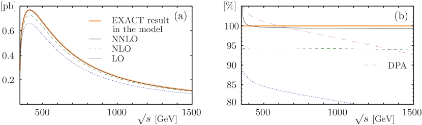
Figure 1: The total cross-section in the model for $t\bar{t}$ production and decay.

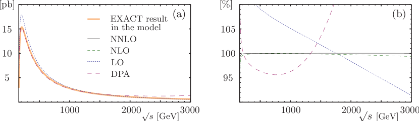
Figure 2: The total cross-section in the model for $W^{+}W^{-}$ production and decay.

                 

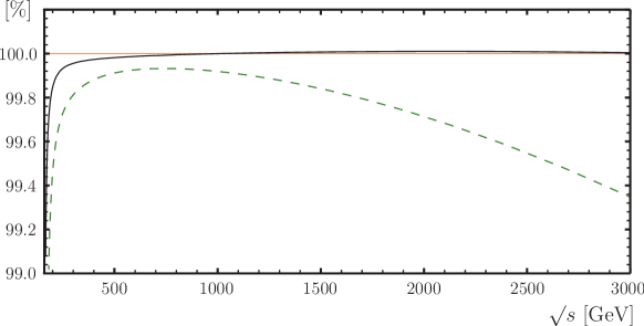
Figure 3: The results of Fig. 2.b with greater scale on vertical axis.

Table 1: $t\bar{t}$ production: the total cross-section in pb and in % with respect to exact result in the model.

$\quad\sqrt{s}$ (GeV)	$\qquad\sigma_{\,\mbox{\tiny EXACT}}\qquad$	$\qquad\sigma_{LO}\qquad$	$\qquad\sigma_{NLO}\qquad$	$\quad\sigma_{NNLO}\qquad$
500	0.6724	0.5687	0.6344	0.6698
	100%	84.6%	94.3%	99.6%
1000	0.2255	0.1821	0.2124	0.2240
	100%	80.8%	94.2%	99.3%
1500	0.1122	0.0867	0.1053	0.1113
	100%	77.3%	93.8%	99.2%

Table 2: $W^{+}W^{-}$ production: the total cross-section in pb and in % with respect to exact result in the model.

$\quad\sqrt{s}$ (GeV)	$\qquad\sigma_{\,\mbox{\tiny EXACT}}\qquad$	$\qquad\sigma_{LO}\qquad$	$\qquad\sigma_{NLO}\qquad$	$\quad\sigma_{NNLO}\qquad$
200	15.258	17.839	15.175	15.235
	100%	116.92%	99.46%	99.85%
500	6.9355	7.5657	6.9294	6.9342
	100%	109.09%	99.91%	99.98%
1000	2.8286	2.9733	2.8263	2.8285
	100%	105.12%	99.92%	100.00%
3000	0.61023	0.55733	0.60625	0.61026
	100%	91.33%	99.35%	100.00%

The outcomes of computations are presented in the Figures and in the Tables. In Fig. 1 in the panels (a) the thick curve shows the behavior of the total cross-section in the model in the case of the top-quark pair production. The dotted, dashed, and continuous thin curves show the results of the MPT computations in the LO, NLO, and NNLO approximations, respectively. It is worth noting that the NNLO result almost coincides with the exact result in the region near and above the maximum of the cross-section. The distinction is visible in the panel (b) where the percentages with respect to the exact result are presented. In Fig. 2 the appropriate results are presented in the case of $W$ pair production. The main difference at Fig. 2 is that already the NLO curve almost coincides with the exact result with the distinction visible in the panel (b) only. In Fig. 2 the appropriate results are presented in the case of $W$ pair production. The main difference at Fig. 2 is that already the NLO curve almost coincides with the exact result with the distinction visible in the panel (b) only. In Fig. 3 the results for NLO and NNLO of Fig. 2.b are repeated with greater scale on vertical axis. In Tables 1 and 2 the outcomes are represented in the numerical form at the characteristic energies at ILC [3]. Note that the relative errors of the computation are less than $10^{-3}$ and $10^{-4}$ in the cases of the top quarks and $W$ bosons, respectively. Therefore the errors are omitted in the data of Tables.

In conclusion, first of all we emphasize that the above results show in practice the existence of the MPT expansion in the case of pair production and decay of fundamental unstable particles. Secondly, the NLO and NNLO approximations in the MPT have very stable behavior at the energies near and above the maximum of the cross-section. The latter result to a large extent is model-independent since it is established in different models. (The latter point is discussed in more details in [12, 13]. Notice also that at lower energies, in particular near threshold, the mode of MPT that has been considered here becomes inapplicable, but there is another mode for MPT [8].) Thirdly, at the ILC energies the NNLO approximation in the MPT give highly satisfactory results in numerical sense. Namely, in the case of the top-quark pair production it gives approximately a half-percent accuracy of the description of the cross-section, and in the case of $W$ bosons does a per-mille accuracy. In fact, this is what is needed at the ILC. So, we conclude that MPT is a good candidate for support at the ILC the pair production and decay of fundamental unstable particles.

References

- [1] W. Beenakker et al., Physics at LEP2 (eds. G.Altarelli et. al., Geneva, 1996) CERN 96-01, Vol. 1, p. 79, hep-ph/9602351; M. Grunewald et al. Four-fermion production in electron-positron collisions. Four-Fermion Working Group (The LEP2-MC workshop 1999/2000), hep-ph/0005309.
-
[2]
A. Denner, S. Dittmaier, M. Roth, L.H. Wieders, Phys. Lett. B612 (2005)
223;
A. Denner, S. Dittmaier, M. Roth, L.H. Wieders, Nucl. Phys. B724 (2005) 247. - [3] J. Brau et al., arXive:0712.1950.
- [4] J. Papavassiliou, A. Pilaftsis, Phys. Rev. Lett. 75 (1995) 3060; D. Binosi, J. Papavassiliou, Phys. Rev. D66 (2002) 111901.
- [5] S. Dittmaier, Proc. of International Europhysics Conference on High-Energy Physics (Jerusalem 1997) p. 709 [hep-ph/9710542].
- [6] F.V. Tkachov, Proc. of the 32nd PNPI Winter School on Nuclear and Particle Physics, St.Petersburg, St.Petersburg, PNPI, 1999, p. 166 [hep-ph/9802307].
- [7] M.L. Nekrasov, Eur. Phys. J. C19 (2001) 441.
- [8] M.L. Nekrasov, Int. Mod. Phys. A24 (2009) 6071.
- [9] M.L. Nekrasov, Plys. Lett. B531 (2002) 225.
- [10] B.A. Kniehl, A. Sirlin, Phys. Lett. B530 (2002) 129.
- [11] M.L. Nekrasov, Proc. of 13th Int. Workshop ACAT, Jaipur 2010, PoS ACAT2010 (2010) 085.
- [12] M.L. Nekrasov, Mod.Phys.Lett. A26 (2011) 223.
- [13] M.L. Nekrasov, Mod.Phys.Lett. A26 (2011) 1807.
-
[14]
V.S. Fadin, V.A. Khoze, Proc. of 24th Winter School of LNPI,
Leningrad, LNPI, 1989, vol. I, p. 3;
D. Bardin, W. Beenakker, and A. Denner, Phys. Lett. B317 (1993) 213;
V.S. Fadin, V.A. Khoze, A.D. Martin and A.Chapovsky, Phys. Rev. D52 (1995) 1377.