The ChaMPlane bright X-ray sources — Galactic longitudes $l=2^{\circ}-358^{\circ}$

Abstract

The Chandra Multiwavelength Plane (ChaMPlane) Survey aims to constrain the Galactic population of mainly accretion-powered, but also coronal, low-luminosity X-ray sources ($L_{X}\lesssim 10^{33}$ erg s^-1). To investigate the X-ray source content in the plane at fluxes $F_{\rm X}\gtrsim 3\times 10^{-14}$ erg s^-1 cm^-2, we study 21 of the brightest ChaMPlane sources, viz. those with $>$250 net counts (0.3–8 keV). By excluding the heavily obscured central part of the plane, our optical/near-infrared follow-up puts useful constraints on their nature. We have discovered two likely accreting white-dwarf binaries. CXOPS J$154305.5$$-$$522709$ (CBS 7) is a cataclysmic variable showing periodic X-ray flux modulations on 1.2 hr and 2.4 hr; given its hard spectrum the system is likely magnetic. We identify CXOPS J$175900.8$$-$$334548$ (CBS 17) with a late-type giant; if the X-rays are indeed accretion-powered, it belongs to the small but growing class of symbiotic binaries lacking strong optical nebular emission lines. CXOPS J$171340.5$$-$$395213$ (CBS 14) is an X-ray transient that brightened $\gtrsim$100 times. We tentatively classify it as a very late-type ($>$M7) dwarf, of which few have been detected in X-rays. The remaining sources are (candidate) active galaxies, normal stars and active binaries, and a plausible young T Tauri star. The derived cumulative number density versus flux ($\log~{}N-\log~{}S$) relation for the Galactic sources appears flatter than expected for an isotropic distribution, indicating that we are seeing a non-local sample of mostly coronal sources. Our findings define source templates that we can use, in part, to classify the $>$10⁴ fainter sources in ChaMPlane.

1. Introduction

The Galactic population of low-luminosity X-ray sources ($L_{X}\lesssim 10^{33}$ erg s^-1) includes normal and active single stars and binaries, pre-main sequence stars, milli-second pulsars, and close binaries containing accreting compact objects (white dwarfs in cataclysmic variables or CVs; neutron stars and black holes in quiescent high- and low-mass X-ray binaries, qHMXBs and qLMXBs). Due to sensitivity constraints of previous surveys, little is known about the distribution of these sources on Galactic scales, or about rare sources for which one needs to sample a large volume to study them as a class. With XMM-Newton and especially Chandra, which combine sensitivity with excellent spatial resolution, existing imaging Galactic X-ray surveys (e.g. Hertz & Grindlay, 1984) can be extended with 2–3 orders of magnitude higher sensitivity down to $10^{-15}$ erg s^-1 cm^-2 and with precise searches for counterparts at other wavelengths. This is what drives several ongoing campaigns, like the XMM-Newton Galactic Plane Survey (XGPS; Hands et al., 2004) and our own Chandra Multi-wavelength Plane survey (ChaMPlane; Grindlay et al., 2005). Such surveys are important for understanding the X-ray emission from galaxies. What was previously observed as a diffuse “band” of X-ray emission along the plane (the Galactic Ridge X-ray Emission or GRXE) has, for a significant part, been resolved into discrete sources (about 50% at 3 keV above $10^{-16}$ erg s^-1 cm^-2 (0.5–7 keV); Revnivtsev et al., 2009). As the GRXE and the diffuse X-rays from non-starbust galaxies have similar properties (Revnivtsev et al., 2008), a substantial point-source component is also implied for the latter. But only in our own Galaxy can we study individual sources, as no observatory in the foreseeable future is able to resolve the faint X-ray emission from other galaxies.

Table 1The sample of bright sources

(1)	(2)	(3)	(4)	(5)	(6)	(7)	(8)	(9)	(10)	(11)	(12)	(13)
CBS	CXOPS J	ObsID-	Date Obs	Texp	$N_{\rm H22,Gal}$	$r_{95}$	$\theta$	Net counts	$F_{\rm X,lim}$	Opt	Other	2XMM J
		aimpoint		ks	cm-2	$\arcsec$	$\arcmin$			ID?	ObsID?
1	$061759.2+222738$	04675-S	04-04-12	58.3	0.22	0.31	1.24	318$\pm$19	5.3	+	$-$	061759.1+222738
2	$102801.4-435107$	03569-S	03-05-23	26.5	0.07	0.40	4.06	258$\pm$17	7.7	+	+	102801.4$-$435106
3	$104814.2-583051$	03842-S	03-10-08	35.5	0.76	0.31	1.03	520$\pm$24	16.0	+	$-$	104814.0$-$583051
4	$111108.1-603657$	02782-S	02-04-08	48.8	1.08	0.52	6.34	331$\pm$20	12.4	+	$-$	$-$
5	$111149.5-604158$	02782-S	02-04-08	48.8	1.15	0.32	2.41	899$\pm$31	12.4	+	$-$	111149.6$-$604157
6	$154204.8-522400$	00090-I	00-04-08	23.6	1.09	0.36	3.24	351$\pm$20	31.9	+	$-$	154205.0$-$522400
7	$154305.5-522709$	00090-I	00-04-08	23.6	1.26	0.53	7.41	669$\pm$27	31.9	+	$-$	154305.5$-$522709
8	$155052.4-562608$	05190-S	03-10-23	47.7	0.58	0.33	2.77	491$\pm$23	10.5	+	+	155052.8$-$562609
9	$155226.8-561704$	01965-S	01-08-18	55.6	0.60	0.37	3.66	360$\pm$20	7.8	+	$-$	155227.1$-$561702
10	$170000.9-265905$	01861-I	01-07-04	32.3	0.14	0.46	7.52	2055$\pm$46	11.6	+	$-$	$-$
11	$170905.5-443140$	04608-I	04-02-01	97.2	0.91	0.63	7.55	299$\pm$19	6.7	+	$-$	170905.5$-$443138
12	$170928.2-442916$	04608-I	04-02-01	97.2	0.89	0.34	2.92	395$\pm$21	6.7	+	+	170928.1$-$442915
13	$170938.2-442255$	04608-I	04-02-01	97.2	0.91	0.46	5.72	362$\pm$20	6.7	$-$	$-$	170938.1$-$442253
14	$171340.5-395213$	05559-I	05-04-19	9.5	1.86	0.32	3.31	1740$\pm$43	117	+	$-$	$-$
15	$171440.6-400234$	00737-I	00-07-25	38.2	1.07	0.68	8.29	356$\pm$21	23.3	$-$	$-$	171440.7$-$400232
16	$171537.1-395559$	00737-I	00-07-25	38.2	1.23	0.40	4.42	327$\pm$19	23.3	$-$	$-$	171537.0$-$395559
17	$175900.8-334548$	04586-S	04-06-25	44.1	0.39	0.38	4.25	546$\pm$24	10.3	+	$-$	175900.7$-$334547
18	$184355.1-035830$	02298-I	01-05-20	96.6	5.82	0.52	7.03	520$\pm$24	20.5	$-$	+	$-$
19	$184421.1-035706$	949-I, 1523-I	00-02-24	94.8	5.70	0.89	9.35	256$\pm$18	23.6	+	$-$	$-$
20	$222833.4+611105$	1948-I, 2787-I	01-02-14	106.2	0.40	0.47	5.49	284$\pm$18	4.8	+	$-$	$-$
21	$235841.7+623437$	02810-I	02-09-14	48.8	0.28	0.56	8.50	1168$\pm$35	9.1	+	$-$	$-$

The main goal of ChaMPlane is to constrain the Galactic distribution of faint accretion-powered sources (mainly CVs); the secondary goal is to do a deep survey of stellar coronal sources. We systematically process Chandra Advanced CCD Imaging Spectrometer (ACIS; Garmire et al., 2003) pointings in the plane to analyze serendipitous detections, and do optical and near-infrared (nIR) follow-up for source classification. Whereas the XGPS studies a specific, approximately 3-deg² region of the plane between Galactic longitudes $l=19^{\circ}$ and 22^∘, ChaMPlane uses archival data without any restrictions on longitude. By now, our coverage is about 7 deg² and encorporates our dedicated surveys of low-extinction bulge regions (“Windows Survey”; e.g. van den Berg et al., 2009; Hong et al., 2009) and of a latitudinal strip around the Galactic center (“Bulge Latitude Survey”; Grindlay et al. 2012, in preparation). Our focus on the bulge is driven by trying to uncover the nature of the thousands of hard inner-bulge sources that are believed to be accreting compact objects—the largest such population in the Galaxy (see e.g. Muno et al., 2009).

Most of our sources are detected with only a few tens of counts or less. Here we want to highlight the brightest ChaMPlane sources, for which we can study the X-ray spectra and light curves in more detail. Not only does this sample include objects that are worth further investigation on their own account, but it also allows us to study the typical content and flux distribution of sources covered by the high-flux end of our survey ($F_{\rm X}\gtrsim 3\times 10^{-14}$ erg s^-1 cm^-2), and define characteristic source types to be used as templates for the many faint sources in our database. Despite our focus on the bulge, for a survey like ChaMPlane this region also has its disadvantages. The high stellar density complicates source identification in the optical/nIR. Moreover, the severe extinction along the line of sight restricts a priori the detection of intrinsically faint (in the optical/nIR) objects like CVs to a few kpc, as illustrated by our CV discoveries in a few central-bulge fields (Koenig et al., 2008). Therefore, we defer the study of our brightest sources towards the central part of the Galaxy to a future paper. Here we exclude the central $\pm$2^∘ around the Galactic center.

In §2 we describe the sample selection and data analysis. We present the sources by class in §3. In §4 we place a few individual sources in a broader context, and consider the sample as a whole. Preliminary results were reported in Penner et al. (2008).

2. Sample selection and data analysis

At this writing, the ChaMPlane X-ray source catalog contains $\sim$15 000 sources from archival ACIS imaging data at Galactic latitudes $|\,b\,|<12^{\circ}$ that meet the primary criteria established in Grindlay et al. (2005): preferably ACIS-I exposures (for the larger field of view) with exposure times $\gtrsim 20$ ks and without bright or extended targets that limit the sensitivity to serendipitous detections. Our preference for fields with a minimal column density $N_{\rm H}$ is almost impossible to realize in the bulge. In §2.1 we summarize the additional criteria adopted to select a bright-source sample, and we explain the X-ray and optical/nIR data analysis in §2.2 and §2.3. General classification guidelines are outlined in §2.4. Cross-correlation of the sample with other X-ray catalogs is described in §2.5.

2.1. Sample selection criteria

Three selection rules define the current sample. First, the number of net counts between 0.3 and 8 keV (our $B_{X}$ band) has to exceed 250 so that a meaningful fit to the X-ray spectrum can be made. Second, to keep positional errors small, a source cannot lie too far from the aimpoint. We only select detections on CCDs I0–I3 and CCD S3 for observations that use the ACIS-I and ACIS-S aimpoint, respectively. For a source with 250 net counts or more, this results in 95% confidence radii that are $\lesssim$ 1$\farcs$0 for aimpoint offset angles up to 10′ (which covers the entire S3 chip and most, i.e. $\sim$92%, of the ACIS-I array) and up to 1$\farcs$6 out to the extreme corners of ACIS-I. Positional errors are estimated using the empirical relation between the 95% confidence radius, net counts, and offset angle presented in Hong et al. (2005), which is based on extensive MARX simulations. Finally, we exclude the region within 2^∘ of the Galactic center (GC) to avoid the most crowded and obscured part of the plane. A total of 63 observations covering 3 deg² satisfy this criterion. Zhao et al. (2005) includes a list of our fields that cover these observations; a few more were added recently, but most of these lie within 2^∘ of the GC and would not have been considered for the present study. The only field that is included here but is not listed in Zhao et al. (2005) is located at ($l$,$b$)=(148.19^∘,+0.81^∘) and was covered by an ACIS-S observation.

Our final sample contains 21 sources from 14 single observations and 2 stacked fields that each consist of 2 overlapping observations added together to increase sensitivity (Hong et al. (2005) give details of our stacking procedure). Table 1 lists the sources in order of increasing right ascension, and summarizes the basic properties. Fig. 1 shows their distribution in the plane. For convenience we use the acronym CBS (ChaMPlane Bright Source) to designate the sources in the text instead of their CXOPS name (column 2 of Table 1).

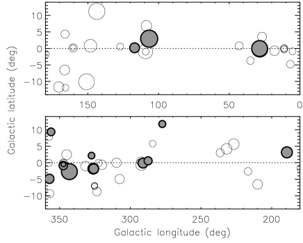
Figure 1.— Distribution of the fields from which we selected the bright sources. Filled circles are the fields that include targets from Table 1. The symbol size scales with the exposure time, which has a maximum GTI value of 106.2 ks.

Table 2Parameters of the best model fits to Chandra spectra

Power-law model
CBS	$\Gamma$	$N_{\rm H,X}$	$Z/Z_{\odot}$	$F_{\rm 0.3-8,u}$	$F_{\rm 2-8,u}$	$\chi^{2}_{\nu}$/d.o.f
		$10^{22}$ cm-2		10-14 erg s-1 cm-2	10-14 erg s-1 cm-2
1	1.7${}^{+0.4}_{-0.3}$	0.7$\pm$0.3	N/A	9.3$\pm$0.6	5.0$\pm$0.3	1.60/12
2	1.9$\pm$0.3	0.15$\pm$0.09	N/A	8.5$\pm$0.6	3.8$\pm$0.3	1.82/8
7	1.0$\pm$0.1	0.2$\pm$0.1	N/A	51$\pm$2	40$\pm$2	0.94/28
9	0.7$\pm$0.3	2.2$\pm$0.8	N/A	21$\pm$1	18$\pm$1	0.93/14
13	2.0$\pm$0.5	6.2$\pm$1.6	N/A	36$\pm$2	16$\pm$1	1.26/15
15	1.9$\pm$0.4	1.5$\pm$0.4	N/A	41$\pm$2	19$\pm$1	0.74/14
16	0.9$\pm$0.3	0.9$\pm$0.6	N/A	23$\pm$1	18$\pm$1	1.29/11
17	0.8$\pm$0.2	1.0$\pm$0.3	N/A	52$\pm$2	43$\pm$2	0.91/23
18	$-$0.26$\pm$0.4	2.1${}^{+1.5}_{-1.3}$	N/A	23$\pm$1	22$\pm$1	1.47/22
Thermal models
CBS	$kT$	$N_{\rm H,X}$	$Z/Z_{\odot}$	$F_{\rm 0.3-8,u}$	$F_{\rm 2-8,u}$	$\chi^{2}_{\nu}$/d.o.f
	keV	$10^{22}$ cm-2		10-14 erg s-1 cm-2	10-14 erg s-1 cm-2
3	0.60$\pm$0.07	0.11$\pm$0.04	0.04$\pm$0.01	10.6$\pm$0.5	0.39$\pm$0.02	0.89/20
4	4$\pm$1	0.22$\pm$0.06	$\equiv$1	7.1$\pm$0.4	3.8$\pm$0.2	1.11/12
5	0.18$\pm$0.02, 0.58$\pm$0.07	0.46$\pm$0.07	$\equiv$1	80$\pm$3	0.24$\pm$0.01	1.10/28
6	0.7$\pm$0.1	0.13$\pm$0.11	0.10${}^{+0.07}_{-0.04}$	17$\pm$1	0.70$\pm$0.04	1.05/11
8	5.5${}^{+2.3}_{-1.3}$	0.25$\pm$0.08	N/A	11.1$\pm$0.5	6.0$\pm$0.3	1.02/18
10	0.31$\pm$0.05, 1.08$\pm$0.04	$<$0.05	0.18$\pm$0.03	67$\pm$1	6.7$\pm$0.2	1.47/57
11	0.9$\pm$0.1	$<$0.07	0.11$\pm$0.06	3.0$\pm$0.2	0.25$\pm$0.02	0.82/10
12	0.8$\pm$0.1	$<$0.18	0.07$\pm$0.05	3.5$\pm$0.2	0.22$\pm$0.01	0.74/12
14	0.9$\pm$0.1, 2.5$\pm$0.3	$<$0.02	0.5${}^{+0.3}_{-0.2}$	340$\pm$8	112$\pm$3	1.01/28
19	4${}^{+2}_{-1}$	0.7$\pm$0.3	$\equiv$1	5.7$\pm$0.4	2.8$\pm$0.2	0.81/10
20	1.0${}^{+0.1}_{-0.2}$	$<$0.29	0.04${}^{+0.06}_{-0.03}$	2.6$\pm$0.1	0.31$\pm$0.02	0.94/6
21	0.79$\pm$0.03	$<$0.02	0.10$\pm$0.02	22.3$\pm$0.7	1.50$\pm$0.05	1.42/41

2.2. X-ray analysis

Hong et al. (2005, 2009) explain the ChaMPlane pipeline for processing the ACIS data. We refer to those papers for details on source detection, and the computation of net source counts and 95% confidence radii on source positions ($r_{95}$). We compute energy quantiles $E_{x}$ following the method described in Hong et al. (2004), which allows us to study the time-resolved spectral properties of our sources.

For each source we create a background-subtracted lightcurve with the CIAO tool dmextract. Counts are extracted from a region that includes 95% of the energy at 1.5 keV; the background is estimated from a source-free annular region centered on the source position. A Kolmogorov-Smirnov (K-S) test on photon arrival times indicates that three sources may be variable (probability for a constant count rate $p_{KS}<1$%). Since the K-S test is only a rough guide to source variability, we follow up with visual inspection of each light curve. We thus identify CBS 7 as a possible fourth variable ($p_{KS}=26$%). The variability of these sources is further discussed in §3.

We use psextract to extract spectra from the same regions used to measure the net source counts, and generate rmf and arf response files for the source and background regions. For the purpose of fitting, spectra are grouped with at least 20 counts per bin in order to use the $\chi^{2}$ statistic. Data that have accumulated in the ChaMPlane archive have been processed with various CIAO versions and calibration files. For consistency, we use the more recently calibrated data from the Chandra archive (processed with CIAO 3.4/CALDB 3.30) for the spectral analysis of all sources. Spectra are fitted within Sherpa version 4.3 to a non-thermal and two thermal models: a power law (the powlaw1d model), thermal bremsstrahlung (xsbremss), and a MeKaL model for an optically-thin thermal plasma appropriate for stellar coronae (xsmekal). For the MeKaL model, we fitted one (1$T$) and two-temperature (2$T$) plasmas, and treated the global metal abundance $Z$ as a fit parameter or fixed it to the solar value. We only adopt the results of the variable-$Z$ or 2$T$ model if fitting for the extra parameters significantly improves the fit; based on this criterion a 2$T$ model turns out to be warranted for 3 sources. We account for an absorbing column density $N_{\rm H}$ using the xsphabs model. For each source, the best-fit model is presented in Table 2. All errors quoted correspond to 68% (1$\sigma$) confidence intervals, computed with the confidence method inside Sherpa. For CBS 20, we report the results of fitting the spectrum of ObsID 2787 only, which constitutes $\sim$95% of the total spectrum.

Table 3Optical and nIR properties of the candidate optical counterparts

(1)	(2)	(3)	(4)	(5)	(6)	(7)	(8)	(9)	(10)	(11)	(12)
CBS	dX-O	dX-O	$N_{\rm ran}$	$V$	$R$	$I$	$H\alpha-R$	$J$	$H$	$K_{s}$	Spectral type
	″	$\sigma$
1	0.19	0.96	0.02	22.9(2)	21.9(1)	20.3(1)	$-0.1(2)$	$\cdots$	$\cdots$	$\cdots$	$\cdots$
2	0.36	1.53	0.04	19.2(1)	18.9(1)	18.4(1)	$0.0(1)$	$\cdots$	$\cdots$	$\cdots$	AGN ($z=1.78$)
3	0.08	0.41	0.04	13.4(1)	12.5(1)	11.7(1)	$0.0(1)$	11.36(2)	10.86(3)	10.69(3)	mid K; ${\rm EW_{H\alpha}}\approx-0.2\pm 0.2$ Å
4	0.25	0.89	0.09	$\cdots$	17.3(1)	$\cdots$	$-0.1(1)$	15.26(6)	14.49(6)	14.29(7)	mid K; ${\rm EW_{H\alpha}}\approx-3.4\pm 0.4$ Å
5	0.16	0.88	0.001	8.09	7.95	7.79	$\cdots$	7.66(3)	7.65(4)	7.62(3)	O7.5III(n)((f))
6	0.42	1.97	0.10	$\cdots$	$\lesssim 17$	$\cdots$	$\cdots$	10.73(3)	10.40(3)	10.35(3)	$\cdots$
7	0.48	1.94	0.17	21.5(1)	20.9(2)	20.3(1)	$-0.5(2)$	$\cdots$	$\cdots$	$\cdots$	$\cdots$
8	0.18	0.86	0.06	14.5(1)	13.3(1)	12.2(1)	$-0.1(1)$	10.43(2)	9.57(2)	9.32(2)	early/mid K, filled-in H$\alpha$?
9	0.31	1.43	0.08	22.5(1)	20.9(1)	19.4(1)	0.0(1)	$\cdots$	$\cdots$	$\cdots$	$\cdots$
10	0.73	2.81	0.16	12.5(1)	$\cdots$	$\cdots$	$\cdots$	9.80(3)	9.13(2)	8.95(2)	$\cdots$
11	0.28	1.00	0.33	$\cdots$	14.0(1)	$\cdots$	$-0.2(1)$	12.23(3)	11.56(4)	11.44(4)	mid/late K; ${\rm EW_{H\alpha}}\approx-1.1\pm 0.3$ Å
12	0.17	0.99	0.13	$\cdots$	12.9(1)	$\cdots$	0.1(1)	11.91(5)	11.58(4)	11.47(3)	early/mid K
14	1.38	2.88	0.50	21.6(1)	18.7(1)	16.6(1)	0.2(1)	13.40(3)	12.56(3)	12.10(3)	$\cdots$
17	0.14	0.62	0.19	15.4(1)	14.0(1)	$\cdots$	$-0.1(1)$	11.01(3)	9.99(3)	9.72(3)	K7–M1 III; ${\rm EW_{H\alpha}}\approx-2.7\pm 0.4$ Å
19	1.34	2.88	0.23	18.0(1)	16.2(1)	14.9(1)	$-0.1(1)$	12.73(3)	11.72(3)	11.04(3)	young star; ${\rm EW_{H\alpha}}\approx-6.6\pm 0.9$ Å
20	0.60	2.25	0.04	15.6(1)	14.8(1)	$\cdots$	$-0.1(7)$	12.93(3)	12.28(3)	12.16(3)	early/mid K; filled-in H$\alpha$?
21	0.49	1.60	0.07	12.2(1)	$\cdots$	11.3(1)	$\cdots$	10.68(2)	10.23(3)	10.14(2)	mid G, early K; filled-in H$\alpha$?

CBS 10 and 14 are piled up by 6% and 30%, respectively. We corrected the count rates accordingly, but the correction for CBS 14 is quite uncertain. To make sure that the spectral fits are not affected by pileup, we excluded events from the central source regions with radius $r$. By trying different values of $r$, we found that $r=1.5$ (CBS 10) and $r=2.0$ (CBS 14) pixels are adequate (i.e. larger values give the same fit results) leaving 90% and 50% of the detected events available for spectral fitting. Energy fluxes were computed by applying the derived count rate-to-flux conversion factors to the pileup-corrected count rates. For CBS 10 the 2$T$ MeKaL fit seems to systematically underestimate the count rate in the highest energy bins between 2 and 4 keV even after removing a large core region. A third, hotter component may be needed to improve the fit.

Column 12 of Table 1 indicates whether a source is detected in a pointing included in our database other than the one listed in column 3. By definition these additional detections have fewer counts. By comparing count rates and energy quantiles (0.3–8 keV) of each detection, we found that CBS 2, 8 and 12 are potentially long-term variables. This is discussed further in § 3.

2.3. Optical/nIR data and analysis

Each ChaMPlane field is imaged through the $VRI$H$\alpha$ filters using the Mosaic cameras on the KPNO-4m and CTIO-4m telescopes. Sequences of deep and shallow exposures provide coverage from $R\approx 12$ to 24 with $S/N\gtrsim 5$. Our values for H$\alpha-R$ colors are defined as the offset from the median H$\alpha-R$ color of all stars in a given field; negative values mark an H$\alpha$ excess flux. We tie the absolute astrometry of the Mosaic images to the International Celestial Reference System (ICRS) using stars in the USNO-A2 (Monet et al., 1998) or 2MASS (Skrutskie et al., 2006) catalogs with rms residuals to the fit of typically $\lesssim 0\farcs 1$. The astrometric solution of Chandra images as a whole can be offset from the ICRS by up to 0$\farcs$7 (90% uncertainty). Without correcting for such a systematic offset, or boresight, positions of X-ray sources could be shifted with respect to those of their true optical counterparts with an amount that is much larger than $r_{95}$, which would harm the optical identification. After correcting for the boresight, we cross-correlate the X-ray and optical source catalogs to look for candidate optical counterparts. The adopted $3\sigma$ search radius takes into account errors on the X-ray and optical positions as well as the boresight error. Zhao et al. (2005) describe the details of our optical imaging campaign, the image processing, computing the boresight correction, and the matching procedure.

ChaMPlane’s spectroscopic campaign is still ongoing. For many of the candidate optical counterparts in Table 1 we have already obtained low-resolution (3–7 Å) optical spectra during various runs conducted between 2002 and 2010 with the FAST spectrograph on the FLWO-1.5m telescope, the IMACS spectrograph on the 6.5m Magellan Baade telescope, and the Hydra spectrographs on the WIYN-3.5m and CTIO-4m telescopes. The spectra are reduced and extracted with a combination of standard IRAF software and dedicated packages. We assign spectral types by comparison with spectral standards observed with a similar resolution (e.g. Jacoby et al. 1984). As a check we run the SPTCLASS code by J. Hernandez, which assigns spectral types by measuring the strength of certain absorption features. Both methods give consistent results.

In summary, of the 21 sources in our sample 17 have candidate optical counterparts, and in each case only a single match is found. Two of these (CBS 5 and 6) have very bright optical matches that are overexposed in the Mosaic images; for CBS 5, we use photometry from the literature. We have optical spectra for 12 of the 17 candidate counterparts. Table LABEL:opt-sample-table lists the properties of all candidate counterparts. The optical/nIR color-color diagrams of Fig. 2 are used for constraining luminosity classes and classifications when optical spectra are not available; see the discussion of individual sources in § 3.

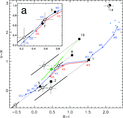
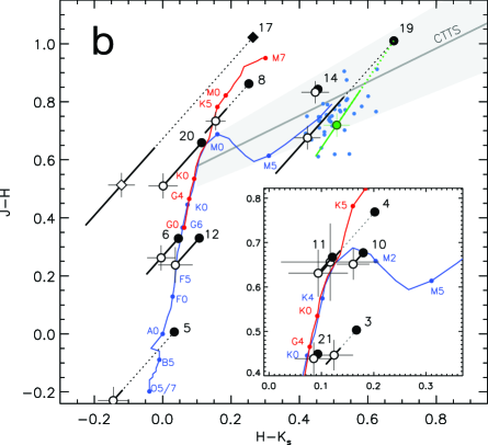
Figure 2.— Optical (left) and nIR (right) color-color diagrams showing the observed colors of the candidate counterparts (filled black symbols) connected with a dotted line to their dereddened colors (open symbols). Error bars are only plotted on the latter. The lengths of the reddening vectors are based on $N_{\rm H,X}$, with the solid thick part of the lines representing the 1-$\sigma$ errors. The slope of the vectors follows the extinction coefficients from Cardelli et al. (1989). As an example of extinction laws that are more appropriate for the bulge, we include (in green) a reddening vector based on Popowski et al. (2003) and Sumi (2004) (for the optical), and Nishiyama et al. (2008) (for the nIR). The gray area in the right panel marks the locus of classical T Tauri stars (CTTS) (Meyer et al., 1997). Circles mark sources we classify as stars, squares are likely AGNs, and diamonds are likely accreting binaries. The counterpart for the candidate AGN CBS 9 is not plotted for clarity. The blue and red lines are the intrisic colors of main-sequence stars and giants, respectively, taken from Johnson (1966), Bessell (1991), and Bessel & Brett (1988). Filled blue circles show the colors of late-type M-dwarfs taken from Henry et al. (2004; spectral types M 8, M 9, M 9.5) and Cruz et al. (2003; spectral types M 9, L 0, L 1). The insets zoom in on crowded regions. See the electronic edition of the Journal for a color version of this figure.

Finding an optical match does not guarantee it is the true counterpart, unless it shows other signs of activity (e.g. excess H$\alpha$ flux) in which case a physical association is very likely. The random-match probability depends on several factors, including the local projected star density and the separation between the X-ray and optical source. To give an idea of the expected number of chance coincidences, we give in column 4 of Table LABEL:opt-sample-table the number of stars expected in the 3$\sigma$ search area based on the optical source density (down to the limiting magnitude of the Mosaic images) within 1′ of the source.

To complement the optical photometry we looked up the $JHK_{s}$ magnitudes of the optical matches in the 2MASS catalog and included them in Table LABEL:opt-sample-table. The quality flags indicate that the $J$ and $H$ magnitudes for CBS 19 are potentially contaminated by an image artifact. This star is also included in the UKIDSS Galactic Planey Survey (GPS) catalog (Lucas et al., 2008); comparison of the $J$ and $H$ magnitudes shows them to be very similar to the 2MASS values with differences in the nIR colors of only $\sim$0.1 mag. None of the other sources appear in the GPS catalog, which covers a limited portion of the plane and is still in progress.

2.4. Source classification

A useful diagnostic to discriminate between stellar coronal sources, accreting binaries, and active galactic nuclei (AGN) is the ratio of the intrinsic and unabsorbed (u) X-ray and optical flux: $\log(F_{\rm X}/F_{\rm O})_{\rm u}=\log F_{\rm X,u}+m/2.5-{\rm ZP}.$ Here, $m$ is the unabsorbed optical magnitude, and ZP is the logarithm of the optical flux for a star with magnitude 0. Assuming a filter width of 1000 Å, the value of ZP is $-5.44$ for the $V$ band, and $-5.66$ for the $R$ band (Bessel et al., 1998). Most coronal sources have $\log(F_{\rm X}/F_{\rm O})_{\rm u}\lesssim-1$, while accretion-powered sources typically have higher values (e.g. Stocke et al., 1991). We note that some CVs, as well as accreting compact objects with massive companions, or qLMXBs with (sub)giant secondaries can have $\log(F_{\rm X}/F_{\rm O})_{\rm u}\lesssim-1$ as well. We use the $B_{X}$ band and the $R$ magnitude where possible, or the $V$ magnitude otherwise, to calculate this ratio. The X-ray flux is obtained from the best spectral fit. X-ray and optical fluxes are corrected for absorption using the column density derived from the X-ray spectral fit ($N_{{\rm H,X}}$).

If we assume that the extinction arises primarily from the Galactic line-of-sight column density, we can use the three-dimensional dust model of Drimmel et al. (2003) to derive distances. These are used in turn to calculate X-ray luminosities $L_{\rm X}$. Distance errors are calculated by inputing the 1-$\sigma$ errors on $N_{\rm H,X}$ to the dust model, and are propagated to estimate errors on $L_{\rm X}$. This approach does not take into account systematic uncertainties in the Drimmel et al. (2003) model that occur even after applying the “rescaling” factors to bring the model closer to the observed COBE/DIRBE far-IR data, which we have done here. To estimate the potential systematic errors in our distances, we have compared the $A_{V}$-versus-distance curves from Drimmel et al. with those from Marshall et al. (2006), available for $|\,l\,|<100^{\circ}$. The Marschall et al. extinction maps have a higher spatial resolution (15′ compared to 35′) and are derived by comparing 2MASS photometry with a Galactic stellar population model. We find that the differences can be large, up to a factor of 2. We note that our assumption that the extinction stems only from the line-of-sight column density is not necessarily justified. For sources that are internally absorbed this assumption can lead to overestimates of the distance, and hence the X-ray luminosity. Furthermore, for sources that lie outside the disk, this method can only provide a lower limit to the distance. Cases for which $N_{\rm H,X}$ is close the asymptotic part of the extinction-versus-distance curve are marked in Table 4, which summarizes our final classification and other derived properties. The errors on $F_{\rm X,u}$ and $\log(F_{\rm X}/F_{\rm O})_{\rm u}$ in Tables 2 and 4 are only based on the errors on the net counts and the magnitude errors, and do not include a contribution from the uncertainties in the spectral fits. In the remainder we assume $N_{\rm H}=(1.79\times 10^{21})\times A_{V}$ cm^-2 (Predehl & Schmitt, 1995). Absolute magnitudes and bolometric luminosities as a function of spectral type are taken from Ostlie & Carroll (2007) unless mentioned otherewise.

Table 4Classification and derived properties for the bright sources

CBS	$d$	$\log L_{\rm X}$	$\log(F_{\rm X}/F_{\rm O})_{\rm u}$	comment
	kpc
Stars
3	1$\pm$0.4	$31.1\pm 0.3$	$-2.50\pm 0.03$	…
4	1.8$\pm$0.3	31.4$\pm$0.2	$-0.93\pm 0.05$	…
5	2.8	32.88$\pm$0.02	$-4.03\pm 0.03$	…
6	0.9$\pm$0.7	31.2${}^{+0.5}_{-1.6}$	$<-0.5$	…
8	3.4$\pm$0.9	32.2$\pm$0.3	$-2.40\pm 0.05$	…
10	$<0.5$	$<31.2$	$-1.84\pm 0.04$	…
11	$<0.6$	$<30.1$	$-2.39\pm 0.05$	…
12	$<1.3$	$<30.8$	$-2.95\pm 0.05$	…
14	$<0.5$	$<32$	$1.64\pm 0.04$	flare star
19	3.0$\pm$0.8	31.8$\pm$0.3	$-2.20\pm 0.05$	…
20	$<3$	$<31.5$	$-2.50\pm 0.05$	…
21	$<0.2$	$<30.0$	$-2.36\pm 0.04$	…
Accreting binaries
7	1.4$\pm$0.1	32.05$\pm$0.08	1.31$\pm$0.07	CV
17	4.9$\pm$0.8	33.2$\pm$0.2	$-1.58\pm 0.04$	symbiotic?
AGN
2	$>2.4$	$>31.8$	$-$0.12$\pm$0.05	…
AGN or accreting binaries
1	$>7.2$	$>32.8$	0.20$\pm$0.05	…
9	$>16$	$>33.8$	$-$2.34$\pm$0.05	…
13	$>11$	$>33.7$	$>-7.6$	…
15	$>23$	$>34.4$	$>0.3$	…
16	$>4.4$	$>32.5$	$>1.1$	…
18	5.8$\pm$2.4	33.0${}^{+0.3}_{-0.5}$	$>-0.9$	…

2.5. Cross-correlation with other X-ray catalogs

Many of our sources have potential counterparts in the XMM-Newton Serendipitous Source Catalog DR3 (Watson et al., 2009). We give the names of sources within 3″ from the Chandra position in column 13 of Table 1. For CBS 7, 14, and 17 we have done a further analysis of the XMM-Newton observations that include these source positions. We have cross-correlated our sample with the ASCA Galactic Plane Survey source catalog (Sugizaki et al., 2001) but found no matches within the 1′ positional uncertainty of the ASCA sources.

3. Results

3.1. Accreting binaries

There is compelling evidence that CBS 7 and 17 are Galactic binaries whose X-rays are powered by accretion onto a compact object, most likely a white dwarf.

3.1.1 CBS 7: a cataclysmic variable

CBS 7 has a hard spectrum that is best fit with a power law with $\Gamma=1.0\pm 0.1$; fits with thermal models only place a lower limit to the plasma temperature of $kT\gtrsim 50$ keV. Photometry of the optical source inside the error circle gives $\log(F_{X}/F_{R})_{\rm u}=1.3\pm 0.1$. The $VRI$ colors of this source are blue compared to the bulk of the surrounding stars, and there is marginal evidence for excess H$\alpha$ emission with H$\alpha-R=-0.5\pm 0.2$. We present optical follow-up spectra that confirm the H$\alpha$ emission lines in CBS 7 elsewhere (Servillat et al., 2011). These characteristics are typical for accreting binaries with compact objects. Using the derived $N_{\rm H,X}$, we find a distance $d=1.2\pm 0.5$ kpc, and an absolute magnitude $M_{V}\approx 10.0$. We conclude that CBS 7 has a low-mass, unevolved donor and is likely a CV rather than a quiescent wind-accreting Be X-ray binary. Sources belonging the latter category can have similary hard X-ray spectra but their massive donors are much brighter in the optical.

The X-ray light curve of CBS 7 is clearly variable, with recurring deep and shallow dips (Fig. 3). We ran a Lomb-Scargle period-search algorithm (Scargle, 1982) on the barycenter-corrected photon arrival times. Hong et al. (2011) give details of the timing analysis. The power-density spectrum between 20 s and 20 000 s shows peaks with $>$99% significance at $P_{1}=4392\pm 290$ s and $P_{2}=8772\pm 957$ s. The longer period corresponds to the spacing of the deep dips, while the shorter one is the spacing between the deep and shallow dips. Figs. 4a and b show the Chandra light curves folded on $P_{1}$ and $P_{2}$. We examined the time-resolved spectral parameters using quantile analysis, but see no indication for variations correlated with count rate. This could be partly due to poor statistics.

CBS 7 is also serendipitously included in an XMM-Newton observation taken on 2003, Aug 14 (ObsID 0152780201; 81 ks). We retrieved the data from the archive and performed further processing with SAS 10.0 following instructions in the XMM-Newton ABC Guide and the SAS Threads. After filtering out time intervals with background flares, $\sim$37 ks (EPIC-PN), 59.2 ks (EPIC-MOS1), and 62.1 ks (EPIC-MOS2) of exposure time remains. Periods consistent with the values of $P_{1}$ and $P_{2}$ show up as significant peaks in the periodograms of the PN light curves. For the MOS1 and MOS2 data only the shorter period is significantly detected, but the folded light curves do not show convincing variability. On the other hand, folding the PN and MOS count rates on $P_{2}$ and $P_{2}/2$ produces light curves that are qualitatively similar to the Chandra light curves and give a smoother result than the periods derived from the XMM-Newton data (Fig. 4c).

To investigate the spectrum, we focused on the data from the PN camera given its larger effective area compared to the MOS cameras and Chandra ACIS at higher energies. We extracted counts from a 20″ source aperture, and corrected for background using a nearby source-free region on the same chip. Fitting a thermal-bremsstrahlung model to the PN spectrum, grouped to have at least 20 counts per bin, sets a lower limit to the temperature of $kT>30$ keV. A power-law fit gives parameters that are consistent with those in Table 2, viz. $\Gamma=1.30\pm 0.06$ and $N_{\rm H,X}=(2.4\pm 0.2)\times 10^{21}$ cm^-2 ($\chi^{2}_{\nu}=1.07$, 91 d.o.f.). The XMM-derived value for $N_{\rm H,X}$ is thus better constrained than the value obtained by fitting the Chandra spectrum, and gives a distance of $1.4\pm 0.1$ kpc; this is the value we include in Table 4. Note however the caveat in §4.1.1 regarding our distance estimate for this source. The residuals show a systematic excess between 6 and 7 keV compared to this model, which prompted us to add a gaussian-shaped emission line at a fixed position of 6.4 keV or 6.7 keV to mimic an Fe K$\alpha$ fluorescent or He-like emission line. While the former does not give sensible line parameters, including a 6.7 keV line removes the systematic residuals. In the latter case, we find a marginal (95%) significance for the presence of the line using the method of Bayesian posterior predictive probability values (e.g.  Protassov et al., 2002). The spectrum can be described by $\Gamma=1.36\pm 0.07$, $N_{\rm H,X}=(2.6\pm 0.3)\times 10^{21}$ cm^-2, and a FWHM of 0.6$\pm$0.2 keV ($\chi^{2}_{\nu}=0.98$, 89 d.o.f.). The unabsorbed flux of $F_{\rm X,u}=6.3\times 10^{-13}$ erg s^-1 cm^-2 (0.3–8 keV) is about 25% higher than found with Chandra.

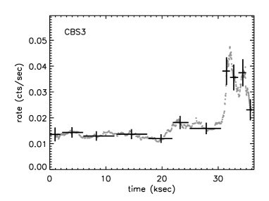
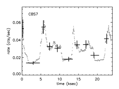
Figure 3.— Background-corrected Chandra light curves of CBS 7 and CBS 3 (0.3–8.0 keV). The points are average count rates in a sliding window with a width that is adjusted to include 50 counts. Error bars are shown for a few representative points where the horizontal error bar marks the bin width.

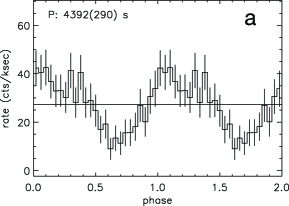
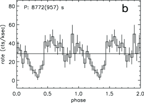
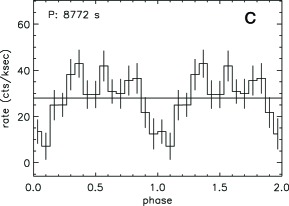
Figure 4.— Left and middle: Chandra light curves for CBS 7 (0.3–8 keV) folded on the periods $P_{1}$ and $P_{2}$ found by the Lomb-Scargle analysis. Right: XMM-Newton EPIC-PN light curve (0.3–8 keV) folded on $P_{2}$. Horizontal lines mark the average count rate.

3.1.2 CBS 17: a symbiotic binary?

CBS 17 is detected $\lesssim$10 pixels away from the chip edge, so we use caution when considering its properties derived from the Chandra data. The hard power-law spectrum ($\Gamma=0.8\pm 0.2$; or $kT>43$ keV for a thermal model) suggests this source is accretion-powered. TiO absorption bands (5847–6058 Å, 6080–6390 Å, 6651–6852 Å) are clearly visible in our Hydra spectrum of the candidate counterpart, and their strength points at a late-K or early-M spectral type. The absence of the gravity-sensitive CaH lines around 6382 and 6389 Å  indicate this star is a giant (Fig. 5). H$\alpha$ is seen in emission, which supports the true association with the X-ray source. On these grounds we conclude that CBS 17 is likely a symbiotic binary where an evolved late-type star transfers mass to a hotter companion, in many cases a white dwarf. Many “canonical” symbiotics are thought of as wind-accreting systems as the strong wind from the evolved companion manifests itself through nebular emission lines excited by the high-energy photons created by the accretion process. We do not see such prominent emission lines in CBS 17. Mass transfer would therefore have to take place through Roche-lobe overflow.

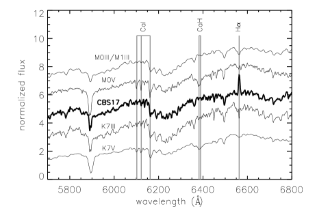
Figure 5.— The optical spectrum of the likely counterpart to CBS 17 (middle; thick line) is compared to template spectra of dwarfs and giants of similar spectral type (Jacoby et al., 1984; Silva & Cornell, 1992) that are reddened with $N_{\rm H}=3.5\times 10^{21}$ cm^-2. Our star clearly shows H$\alpha$ emission. The vertical lines mark CaI (6102, 6122, 6162 Å) and CaH (6382, 6389 Å) lines that are prominent in dwarfs but weak or absent in giants and in CBS 17.

The observed nIR colors of CBS 17 are only consistent with the spectral classification if the extinction is lower ($N_{\rm H}\approx 3\times 10^{21}$ cm^-2) than the one derived from X-ray spectral fitting (Fig. 2b). A lower value for $N_{\rm H}$ of about $3.5\times 10^{21}$ cm^-2 is also suggested by comparing the continuum slope of the Hydra spectrum to artificially reddened template spectra. Formally the error bar on $N_{\rm H,X}$ allows such low values (the difference is $\sim$2.3 $\sigma$), but the discrepancy can also indicate that there is material inside the system obscuring the X-ray emitting region but not the late-type giant. Therefore, we do not use $N_{\rm H,X}$ to estimate a distance, but adopt $N_{\rm H}=(3.25\pm 0.25)\times 10^{21}$ cm^-2 to calculate a spectroscopic distance based on the allowed range of spectral type. A K7 III giant has $M_{V}=+0.4$, while an M1 III giant has $M_{V}=-0.2$, resulting in $d=4.1-5.6$ kpc, and $\log L_{\rm X}=33.2\pm 0.2$.

CBS 17 is included in three XMM-Newton observations. It is commented on by Angelini & White (2003, AW03; their source 1) as a serendipitous detection and possible AGN that stands out in a 6.2–6.8 keV Fe-band image of the first of these observations. Kaaret et al. (2006) also list CBS 17 among the serendipitous detections in the first and second XMM-Newton observation, as well as in the Chandra observation analyzed here. Their reported fluxes indicate long-term variability but are based on the assumption (for all their sources) of a power-law spectrum with $\Gamma=1.5$ and $N_{\rm H}=3.1\times 10^{21}$ cm^-2. This motivated us to do a more detailed analysis. Table 5 lists all X-ray observations for CBS 17.

Table 5X-ray observations of CBS 17 used in our analysis

epoch	telescope/instrument	ObsID	Date Obs	Texp
				ks
1	XMM-Newton/EPIC-PN	0032940101	2001-03-08	15.4
2	Chandra/ACIS-S	04586	2004-06-25	44.1
3	XMM-Newton/EPIC-PN	0203750101	2004-09-18	42.7
4	XMM-Newton/EPIC-PN	0500540101	2008-03-15	44.6

We extracted spectra following the same procedures as for CBS 7, and restricted the analysis to the EPIC-PN data. First we fitted each spectrum individually. The results, summarized in the upper part of Table 6, indicate spectral and/or flux variability but the errors are large. Therefore we also tried fitting all spectra simultaneously, forcing various combinations of parameters to be the same for each epoch. Keeping $N_{\rm H,X}$ and the power-law slope and normalization the same gives an unacceptable fit with $\chi^{2}_{\nu}=1.81$ and 278 d.o.f. for the overall fit, which confirms the variability. Allowing only $N_{\rm H,X}$ to vary for each epoch does not result in a good fit either (overall $\chi^{2}_{\nu}=1.69$, 275 d.o.f.). The same is true if we fix $N_{\rm H,X}$ and $\Gamma$, but allow the normalization to vary; in this case an unsatisfactory fit is found for epoch 1 and 2. If we let $\Gamma$ and the normalization vary and keep $N_{\rm H,X}$ the same, a good fit is found for each epoch (Table 6, bottom). In this case we see small variations of $\Gamma$, and the intrinsic flux varies up to $\sim$60%. The largest flux change is seen between two XMM-Newton observations (epoch 1 and 3), so this finding is unaffected by the fact that CBS 17 lies close to the chip edge in the Chandra observation.

Fig. 6 shows the data and best model fits for fixed $N_{\rm H}$. The spectrum from epoch 1 shows small positive residuals between 6 and 7 keV that could correspond to the Fe K line reported by AW03. The good fits achieved with models without an Fe K line do not warrant adding such an emission component. When we do include a gaussian-shaped emission line, we find parameter values that are consistent with the results of AW03, viz. 6.24$\pm$0.15 keV and 0.66$\pm$0.24 keV for the line center and width, $\Gamma=1.7\pm 0.2$, $N_{\rm H,X}=(0.9\pm 0.2)\times 10^{22}$ cm^-2, and $F_{\rm X,u}=4.8\times 10^{-13}$ erg s^-1 cm^-2 ($\chi^{2}_{\nu}=0.91$ for 39 d.o.f.). Here we re-grouped the spectrum to $\geq$15 (instead of 20) counts per bin for a slightly better resolution. Only the spectrum from epoch 1, during which the source was at its softest, shows a hint of a line. The absence of this line in the Chandra data could be due to the poorer sensitivity at higher energies.

Follow-up studies are needed to uncover the nature of CBS 17. With high-resolution optical spectroscopy the binary status can be established, and the orbital period and companion masses can be constrained. To test if the companion is (close to) Roche-lobe filling, one can look for the signature of a distorted companion in the optical/nIR light curves.

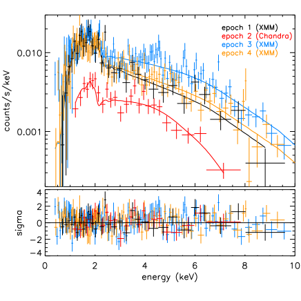
Figure 6.— Chandra and XMM-Newton spectra of CBS 17 are shown together with the best fitting model to the data. Solid lines are the model fits for an absorbed power law with the column density $N_{\rm H,X}$ kept the same for each epoch. The model parameters are listed in the bottom part of Table 6. See the electronic edition of the Journal for a color version of this figure.

Table 6X-ray spectral fits for CBS 17

epoch	$\Gamma$	$N_{\rm H,X}$	$F_{\rm X,u}\times 10^{-13}$	$\chi^{2}_{\nu}$/d.o.f
		1022 cm-2	erg s-1 cm-2
each spectrum fit individually
1	1.42$\pm$0.16	0.76$\pm$0.16	4.2	1.02/30
2	1.0$\pm$0.3	0.8$\pm$0.2	5.2	0.91/23
3	0.87$\pm$0.07	0.70$\pm$0.10	6.6	1.08/120
4	1.19$\pm$0.08	0.66$\pm$0.10	4.1	0.93/96
same $N_{\rm H,X}$ for each epoch
1	1.38$\pm$0.10	0.71$\pm$0.06	4.1	1.00/272
2	0.64$\pm$0.10	.	5.0	.
3	0.87$\pm$0.06	.	6.6	.
4	1.23$\pm$0.07	.	4.2	.

3.2. Stellar coronal X-ray sources

We classify 9 sources (CBS 3, 4, 5, 6, 10, 11, 12, 20, 21) as stars or active binaries based on the following criteria: $\log(F_{\rm X}/F_{\rm O})_{\rm u}\lesssim-1$ (Koenig et al., 2008, and references therein), the X-ray spectrum is well fit by a thermal model, and the corresponding plasma temperature $kT$ is a few keV at most. Their properties are described in §3.2.1 (late-type stars) and §3.2.2 (early-type star). Three exceptional cases—CBS 19, 8, and 14—are discussed in §3.2.3–3.2.5.

3.2.1 Normal and active late-type stars

Our optical spectra show that CBS 3, 4, 11, 12, 20 and 21 are G or K stars (Table LABEL:opt-sample-table). We have not obtained spectra for the candidate counterparts to CBS 6 and 10, yet. Considering their dereddened 2MASS colors, they are probably late-type stars as well, with spectral types around early G and early M, respectively (Fig. 2b). The X-rays of late-type stars are emitted by a hot coronal plasma, which is confined by magnetic fields that are generated by a solar-like dynamo operating in the convective outer layers. See Güdel (2004) for a review.

The X-ray derived extinction values for these eight stars are all relatively low, and consequently the Drimmel extinction-versus-distance curves place them nearby. Our estimates or upper limits on $L_{X}$ are consistent with X-ray luminosities of nearby F–K stars ($\log L_{\rm 0.1-2.4~{}keV}\approx 26.5-29.5$; Schmitt & Liefke, 2004) and active binaries ($\log L_{\rm 0.1-2.4~{}keV}\approx 28-32$; Dempsey et al. 1993, 1997) as measured by ROSAT, and of active binaries in open clusters ($\log L_{\rm 0.3-7~{}keV}\approx 28-31$; van den Berg et al., 2004) as measured by Chandra. If we adopt the $N_{\rm H,X}$-derived distances to calculate absolute magnitudes $M_{V}$ or $M_{R}$, we find that CBS 4, 10, 11, and 21 are likely main-sequence stars or BY Dra-type active binaries, and CBS 3 is likely a subgiant or an RS CVn-type active binary. CBS 12 and 20 are dwarfs or subgiants, either single or in an active binary. While one should be wary when using our $N_{\rm H,X}$-derived distance estimates, we note that these sources are relatively nearby, and that non-flaring active stars or binaries are often not internally absorbed. Low-resolution stellar X-ray spectra are often found to be better fit with a sub-solar coronal metal abundance $Z$ than with a solar abundance (Güdel, 2004). We also see this in the results of our fits to the spectra of CBS 3, 6, 10, 11, 12, 20, and 21.

With $kT\approx 4$ keV and $\log(F_{\rm X}/F_{R})_{\rm u}\approx-0.9$, CBS 4 appears to be more active than most of the sources in this category, which have $kT\lesssim 1$ keV. Here we could be seeing the effect of a coronal flare during the first $\sim$20 ks of the observation. To study temporal variations in the energy spectrum of CBS 4, we resort to quantile analysis as there are too few counts to fit, and compare, spectra extracted from different sub-intervals of the exposure. In quantile analysis, the energy values that divide the energy distribution of the photons in certain fixed fractions are used as spectral diagnostics. This approach is more powerful than measuring the number of counts in fixed energy bands (as is done when using hardness ratios), as the errors on the diagnostic are less sensitive to the underlying spectral shape. Following Hong et al. (2004) we choose the median energy ($E_{50}$), and the 25% and 75% quartiles ($E_{25}$, $E_{75}$) to characterize the spectra. By comparing the observed quantiles with those expected for a spectral model of choice, the X-ray spectral parameters and $N_{\rm H,X}$ can be constrained. As expected for a coronal flare, the spectrum of CBS 4 is harder when it is bright compared to quiescence, where the spectrum can be described by $\sim$1 keV thermal plasma. For intermediate count rates ($\sim$10 cts ks^-1) the source moves down in the quantile diagram which is the signature of two different temperatures contributing more or less equally. Flaring has been frequently observed in M dwarfs, but also in earlier-type dwarfs (see Güdel 2004 and references therein). What is puzzling is the trend of spectral hardening towards the end of the observation, when the count rate is at its lowest.

CBS 3 is also an X-ray variable, showing a flare-like event near the end of the exposure (Fig. 3). We see no indication for a change in its X-ray spectrum during the flare.

CBS 12 is potentially a long-term variable. Besides in the observation we analyze here, it is detected in ObsID 757 (2000 Aug 14, 13.4 ks GTI) with a significantly higher count rate: 9.8$\pm$1.2 versus 4.3$\pm$0.2 cts ks^-1. The energy quantiles in the two ObsIDs are consistent.

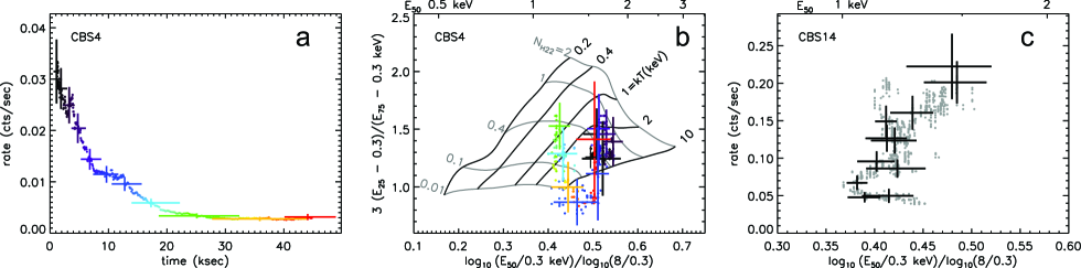
Figure 7.— Left: Background-corrected Chandra light curve of CBS 4 (0.3–8.0 keV). See the caption of Fig. 3 for a description of the binning. Middle: Time-resolved quantile diagram (0.3–8 keV) for CBS 4. Each point corresponds to the bin of the same color in the left panel. The points are plotted on a thermal-bremsstrahlung grid, where the black lines represent a constant temperature $kT$ and the gray lines represent a constant column density $N_{\rm H}$ (in units of 10²² cm^-2). By comparing the observed quantiles with these grid lines, one can constrain the spectral parameters for this assumption of spectral model. A clear concentration towards two temperatures is seen. Note that the spectrum appears to become harder again in the last two time bins when the count rate is low. Right: The 0.3–8 keV count rate for CBS 14 shows an overall positive correlation with spectral hardness. Events from the piled-up core are excluded. See the electronic edition of the Journal for a color version of this figure.

3.2.2 CBS 5: an early-type star

The bright star that is matched to CBS 5 is HD 97434. The O7.5III classification by Walborn (1973) is in better agreement with our Hydra spectrum than other classifications found in the literature. Using its colors and spectral type, Vazquez & Feinstein (1990) derive $A_{V}=1.5\pm 0.2$ and $M_{V}=-5.7\pm 0.15$, where the errors were estimated by us (since none were given by Vazquez & Feinstein) and set to reasonable values based on the information provided in their study, and the compilation of absolute magnitudes of O stars in Vacca et al. (1996). This gives a distance to CBS 5 of $d=2.8\pm 0.4$ kpc. The X-rays from single early-type stars are believed to arise from shock-heated plasma formed by instabilities in the strong winds emanating from such massive stars. The spectra can be described by the combination of two thermal components with $kT\approx 0.3$ and 0.7–1 keV (Güdel & Nazé, 2009). This agrees with our results. We find $\log(F_{\rm X}/F_{R})_{\rm u}\approx-4.0$, and $\log(L_{\rm X}/L_{{\rm bol})}\approx-6.3$ (for $d=2.8$ kpc), also typical for O stars.

Bhatt et al. (2010) analyzed XMM-Newton data of HD 97434 taken two months before the Chandra observation. To facilitate comparison, we fit our spectrum with their adopted model, i.e. a 2$T$ APEC thermal plasma model (xsapec). Our data are not good enough to constrain $Z$. Setting $Z/Z_{\odot}\equiv 0.21$, i.e. the value found by Bhatt et al, we find $N_{\rm H,X}$ $=(3\pm 1)\times 10^{21}$ cm^-2, $kT_{1}=0.24\pm 0.05$ keV, and $kT_{2}=0.6\pm 0.1$ keV, suggesting no change in these parameters between the epochs. Bhatt et al. assume that HD 97434 is a member of the open cluster Trumpler 18 located at 1.55$\pm$0.15 kpc (Vazquez & Feinstein, 1990). However, the spectroscopic distance (see above) places it behind the cluster by $\sim 3\sigma$. When adopting a common distance, the Chandra luminosity is 2–3 times lower than the XMM-Newton value, indicating long-term variability.

3.2.3 CBS 19: a pre-main sequence star

The temperature derived for CBS 19 ($kT=4^{+2}_{-1}$ keV) indicates a high level of activity. Our Hydra spectrum of the candidate counterpart shows a clear H$\alpha$ emission line with EW=$-$6.0$\pm$0.8 Å. At the poor signal-to-noise ratio of our spectrum, the continuum looks featureless except for the Na I D doublet around 5890 Å, which could be interstellar in nature. This makes spectral classification challenging. At first sight, the optical and nIR colors of the candidate counterpart seem to disagree (Fig. 2). The former suggest a spectral type of late-F to early-M, whereas the latter point at a late-M star. Such cool M stars show prominent TiO absorption bands in their optical spectra but these are notably absent in CBS 19.

One explanation is that CBS 19 is a young, pre-main sequence (PMS) star surrounded by a warm, circumstellar disk that causes excess nIR emission. In fact, after accounting for the extinction derived from $N_{\rm H,X}$, the location of CBS 19 in the nIR color-color diagram (Fig. 2b) agrees with the locus of the classical T Tauri stars (CTTS), a sub-class of PMS stars that are still actively accreting from their circumstellar disk (Meyer et al., 1997). The prominent but relatively weak (compared to CVs) H$\alpha$ emission is also in line with this classification. The X-ray properties of CBS 19 are typical for PMS stars, where X-rays are generated by a high level of magnetic activity, with a possible contribution of (relatively soft) X-rays from the accretion process (e.g. Feigelson et al., 2007). We note that the disk can be a source of local extinction, and therefore our estimates of the distance ($d=3.0\pm 0.8$ kpc) and luminosity ($\log L_{\rm X}=31.8\pm 0.3$ erg s^-1) based on the Drimmel model may be too high.

The Li I 6708Å line is a well-known indicator of youth. Detection of this line in high-resolution optical spectra of CBS 19 would confirm its T Tauri nature.

3.2.4 CBS 8: an RS CVn binary

Our Hydra spectrum of the candidate counterpart to CBS 8 classifies it as an early/mid K star. The X-ray spectrum of CBS 8 is rather hard for steady, stellar coronal emission. For a power-law model we find $\Gamma=1.9\pm 0.2$; for a bremsstrahlung model we find $kT=5.5^{+2.3}_{-1.3}$ keV. The count rate is stable throughout the 48-ks observation, so it is unlikely that the hard spectrum is the result of a typical coronal flare which can have a decay time of up to $\sim$15 ks (Güdel, 2004). CBS 8 appears in our database four more times, always with a lower count rate (at a level of $>$3 $\sigma$). The largest difference is found with respect to ObsID 3807 (2002 Sep 24, 23 ks GTI) where the source is detected with 2.7$\pm$0.4 cts ks^-1 compared to 10.7$\pm$0.5 cts ks^-1 in the observation analyzed here, taken a year later. In ObsID 3807 the source appears softer, with $E_{50}=1.2\pm 0.1$ keV compared to $E_{50}=1.64\pm 0.04$ keV. The hardening and brightening of the source could point at an increased level of coronal activity occurring on a $\sim$year time scale.

The distance derived from $N_{\rm H,X}$ gives an absolute magnitude $M_{V}=0.4^{+1.2}_{-0.9}$, pointing to the star being a luminosity-class III giant (for a K3 III star, $M_{V}=+0.8$). Also from Fig. 2 it can be seen that the spectral type better agrees with the optical/nIR colors if we assume the star is a giant instead of a dwarf. The H$\alpha$ absorption line is very weak, a sign that the line may be filled in by excess H$\alpha$ emission. We tentatively classify CBS 8 as an active RS CVn-type binary.

3.2.5 CBS 14: an ultracool dwarf?

The X-ray spectrum of CBS 14 is well fitted with a 2$T$ MeKaL model with $kT_{1}\approx 0.9$ keV and $kT_{2}\approx 2.5$ keV, and minimal absorption ($N_{\rm H,X}<2\times 10^{20}$ cm^-2). Apart from small-amplitude variations, the count rate steadily declines during the $\sim$9.5 ks observation. The spectrum becomes softer when the source gets fainter (Fig. 7). This is typical for a coronal flare, but since the source was already bright at the start of the observation it is impossible to say if the light curve shows the characteristic “fast rise, slow decay”-profile of a flare.

The error circle of CBS 14 contains an extremely red object with $V-K_{s}=9.4$. Its optical/nIR colors place this object among the dwarfs with spectral type M 7 or later; these are the so-called ultracool dwarfs. This is illustrated in the color-color diagrams of Figs. 2 and 8, which also include nearby ultracool dwarfs. By comparing its $J$ magnitude, and $I-J$ and $J-K_{s}$ colors with those of ultracool dwarfs at known distances (Phan-Bao et al., 2008), we estimate an approximate spectral type of M 9 and $d\approx 24$ pc.

The area around CBS 14 is included in the field of view of the EPIC-MOS cameras in two XMM-Newton observations: 0093670501 (2001 Mar 2; 14 ks) and 0207300201 (2004 Feb 22; 34 ks); the source lies outside the field of the EPIC-PN camera. After filtering out background flares, $\sim$13 ks and $\sim$15 ks of exposure time remain. No source is seen at the location of CBS 14. Upper limits on the flux are estimated by first extracting all counts (0.3–8 keV) from within 20″ of the Chandra source position. Using Gehrels (1986), we compute the 3-$\sigma$ upper limit on the number of counts. The background contribution is estimated from an annulus around the source position. The resulting limit on the net source counts is converted to a count rate limit using the value of the exposure map at the source position. With the spectral model of Table 2, we estimate that the most restrictive 3-$\sigma$ flux limit comes from the 2001 observation and is $\sim$1.6 $\times$ 10^-14 erg s^-1 cm^-2. It is possible that the spectrum is softer when the source is not flaring, but for a $kT=0.5$ keV MeKaL spectrum the upper limit on the flux changes only 10%. The flux from the Chandra observation is uncertain due to the pileup. A conservative lower limit is obtained by assuming that the detected count rate is the incident count rate. This implies an unabsorbed flux of $>1.6\times 10^{-12}$ erg s^-1 cm^-2 (0.3–8 keV), meaning that CBS 14 was $\gtrsim$100 brighter during the Chandra observation compared to the time of the XMM-Newton observations. Therefore, our estimate of $(F_{\rm X}/F_{\rm O})_{\rm u}$ is very uncertain as our X-ray and optical observations were not simultaneous.

CBS 14 was not detected in the ROSAT All Sky Survey. The detection limit of $\sim$0.015 cts s^-1 (0.1–2.4 keV, Huensch et al., 1998) gives an upper limit to the intrinsic flux of $\sim$1.7 $\times$ 10^-13 erg s^-1 cm^-2 for a $kT=0.5$ keV MeKaL model and $N_{\rm H,X}=2\times 10^{20}$ cm^-2. The lower limit to the Chandra flux is $1.4\times 10^{-12}$ erg s^-1 cm^-2 when extrapolated to the ROSAT band, implying a flux increase of at least a factor of $\sim$8.

Spectroscopic follow-up is needed to test our tentative classification of CBS 14 as an ultracool dwarf. It is not obvious what an alternative explanation could be. The X-ray spectrum points at negligible extinction and excludes the option of a background AGN or a heavily-obscured object to explain the red optical/nIR colors. The number of random interlopers inside the area searched for counterparts is $N_{\rm ran}=0.5$, so there is a reasonable chance that the red object is a chance coincidence. This implies that the true counterpart has $R>24$.

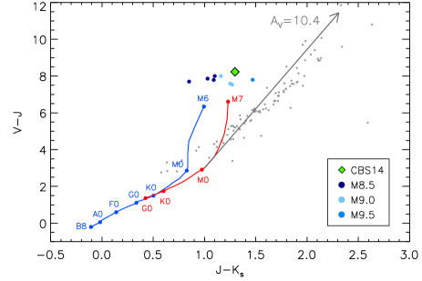
Figure 8.— Color-color diagram illustrating the tentative classification of CBS 14 as a very late-type dwarf based on the optical/nIR colors of its candidate counterpart (green diamond). For comparison we include the intrinsic colors of main-sequence stars as a black (blue) curve, of giants as a light gray (red) curve, and nearby ($\lesssim$30 pc) ultracool dwarfs (filled circles; Henry et al. (2004)). Most stars in a 5′ $\times$ 5′ region centered on CBS 14 (grey dots) lie along the reddening vector (Nishiyama et al., 2008), shown with a length representing the total Galactic extinction in this direction ($A_{V}=10.4$). The candidate counterpart to CBS 14 lies away from this vector among the nearby ultracool dwarfs. Classification as an ultracool dwarf is consistent with the low extinction ($N_{\rm H,X}\lesssim 2~{}10^{20}$ cm^-2 or $A_{V}\lesssim 0.1$) found from the X-ray spectrum. Errors on the colors of CBS 14 are smaller than the symbol size. See the electronic edition of the Journal for a color version of this figure.

3.3. AGN

Based on its optical spectrum, we classify CBS 2 as an AGN. Broad emission lines, coming from gas moving at high speeds around the central supermassive black hole, are prominently visible and constrain the redshift to $z\approx 1.78$. Our database includes two detections of CBS 2: the one analyzed here and a detection in ObsID 835 (2000 Jan 5; 26.5 ks GTI), in which the source is about half as bright (4.9$\pm$0.5 versus 10$\pm$0.7 cts ks^-1). The energy quantiles are consistent.

3.4. AGNs or Galactic accreting binaries

The relatively hard X-ray spectra of CBS 1, 9, 13, 15, 16, and 18 suggest that their X-rays are accretion-powered, but with the information we have we cannot distinguish between AGNs or Galactic sources. The spectra of most AGNs can be described by power laws with photon spectral index $\Gamma\approx 1-2.5$ (see e.g. Tozzi et al., 2006). The spectra of our sources have photon indices that lie in this range, except for CBS 18 (see below).

The large errors on $N_{\rm H,X}$ make it difficult to constrain the distances, as the $N_{\rm H,X}$ values are consistent with the total Galactic column densities $N_{\rm H,Gal}$ towards these sources at the $<$2.5$\sigma$ level. Therefore, for these sources we can only derive lower limits to the distance. Only for CBS 13 does $N_{\rm H,X}$ exceed $N_{\rm H,Gal}$ by $>$3$\sigma$; but while an AGN nature is the most obvious explanation, one cannot exclude it is a highly-obscured Galactic source.

For CBS 1 and 9 we have candidate optical counterparts, but no optical spectra to classify them. The H$\alpha-R$ colors show no indication of an excess H$\alpha$ flux. Whereas the spectra of most CVs and quiescent X-ray binaries show clear H$\alpha$ emission (e.g. Torres et al. 2004), some qLMXBs have H$\alpha$ emission lines with equivalent widths $>-10$Å (e.g. Elebert et al. (2009)). Such weak lines are not expected to make the H$\alpha-R$ color stand out (see Fig. 4 in Zhao et al. (2005)). We also note that our method to look for H$\alpha$ excess sources only works for redshift $z=0$, and fails for objects at significantly higher redshifts. Follow-up spectroscopy of the candidate counterparts is necessary for an unambiguous classification. CBS 13, 15, 16, and 18 have no candidate optical counterparts down to the limiting magnitude of our Mosaic images. The (limits on the) $\log(F_{\rm X}/F_{R})_{\rm u}$ values of all six sources are consistent with both a Galactic and an extra-galactic interpretation (e.g. Hornschemeier et al., 2001).

For CBS 18 $N_{\rm H,X}$ is relatively low compared to $N_{\rm H,Gal}$ (($2.1\pm 1.5)\times 10^{22}$ cm^-2 versus $5.8\times 10^{22}$ cm^-2), and it may be the best candidate among this subset to be an accreting binary. The spectral fit gives an unusually flat photon index ($\Gamma=-0.3\pm 0.4$), and there is a hint of a systematic trend in the residuals above 5 keV. The data are of insufficient quality to test for the presence of an emission line, which is not included in our model but could skew the spectrum to seem flatter than it actually is.

CBS 18 is also detected in the consecutive Chandra observations 949 (42 ks) and 1523 (58 ks) from 2000 Feb 24/25. The energy quantiles and count rates are consistent in all observations. The combined light curve from ObsIDs 949 and 1523 shows a weak sign of periodicity at $P=503\pm 1$ s, with the corresponding peak in the Lomb-Scargle periodogram just above the 99% confidence level. As the folded light curve does not look convincingly variable, we consider this detection marginal at best. There is no sign of periodicity in the light curve from the observation analyzed here.

CBS 18 lies in the field observed by Ebisawa et al. (2005) and is their source # 200 or CXOGPE J184355.1-035829. Ebisawa et al. did not find a counterpart in the nIR follow-up campaign, which is complete down to $J=18$, $H=17$, and $K_{s}=16$. The lack of a counterpart implies $\log(F_{\rm X}/F_{K_{s}})_{\rm u}>0.17$, which also points at an accretion-powered source.

4. Discussion

Our sample of 21 bright sources consists of 12 stars and 9 accretion-powered sources. Except for CBS 5, the stars are coronal emitters where magnetic fields play a major role in developing or sustaining hot plasmas. Among the accreting sources, two are Galactic binaries (CBS 7 is a CV; CBS 17 is a candidate symbiotic binary), CBS 18 could be a CV, one is a confirmed AGN, and for the remaining six this distinction is less clear. We first discuss three of our bright sources in a broader context, and then continue to consider our sample as a whole.

4.1. Individual systems

4.1.1 CBS 7: a likely magnetic cataclysmic variable

The hard spectrum of CBS 7 suggests it is a magnetic CV (e.g. Heinke et al., 2008), although some dwarf novae in quiescence have hard spectra as well (e.g. Balman et al., 2011). Magnetic CVs can be divided in two subclasses. In polars, the magnetic field is strong enough ($B\gtrsim 10$ MG) to lock the spin to the orbital motion. Intermediate polars (IPs) have fields of moderate strength ($B\approx 1-10$ MG), which are too weak to force synchronism. It is not clear which of these classes CBS 7 belongs to. Our follow-up optical and nIR data indicate that the longer of the two X-ray periods is likely the orbital period ($P_{b}$) and we refer to Servillat et al. (2011) for a detailed discussion. The origin of the shorter period is less clear. If the system is synchronized, the variability could be caused by the two poles or accretion spots on the white dwarf being partially (self)eclipsed. If the system is asynchronous, the shorter period could reflect the white-dwarf spin period ($P_{s}$), which would then be half the orbital period by chance. The ratio of the periods ($P_{s}\approx 0.5P_{b}$) is relatively high compared to the typical ratio for IPs; most have $P_{s}\lesssim 0.3P_{b}$. It would add CBS 7 to a small but growing number of “near-synchronous” IPs that may be evolving towards synchronism (Norton et al., 2008; Hong et al., 2011). As the X-ray spectral properties of CBS 7 do not vary with count rate, the dips are likely not caused by a variation of the local amount of absorbing material. It is not uncommon for magnetic CVs to be internally absorbed, which can cause our distance and $L_{\rm X}$ estimates to be overestimated.

4.1.2 CBS 17: a new hard X-ray emitting symbiotic?

Traditionally, symbiotic binaries were thought of as soft X-ray emitters. This picture was mostly based on ROSAT observations that were limited by its soft response (Mürset et al., 1997). Recently, an increasing number of symbiotics has been detected at harder energies (Kennea et al., 2009; Luna et al., 2010; van den Berg et al., 2006). Kennea et al. (2009) suggest that for RT Cru, T CrB, CD$-$57 3057, and CH Cyg the hard X-rays are thermal and come from an accretion-disk boundary layer around a massive, non-magnetic white dwarf. The potentially high white-dwarf masses makes them interesting as candidate SN Ia progenitors. CBS 17 could be a member of this class of “hard” symbiotics. Besides the hard spectrum, similarities with this class include the weak optical emission lines and possibly an internal absorption component. On the other hand, our analysis suggests that the long-term variability is not caused by variations in the column density, whereas in the systems discussed by Kennea et al. (2009) the variations were found to result from variations in the intrinsic absorption.

4.1.3 The candidate ultra-cool dwarf CBS 14

Unlike earlier-type M stars that have a radiative core and convective envelope, ultracool dwarfs are fully convective with cool and effectively neutral atmospheres. Multi-wavelength diagnostics indeed mark a change in magnetic activity around spectral type M 7, but a larger sample is needed to get a clearer picture: only 12 ultracool dwarfs have been detected in X-rays (Berger et al., 2010; Robrade et al., 2010). In this context, it is important to establish the nature of CBS 14. Its colors place it between the M 9 and L 0 dwarfs. So far, there is no firm X-ray detection of a dwarf later than M 9; the L 2-dwarf Kelu-1 with a marginal detection of 4 photons is the only possible exception (Audard et al., 2007). With $\log L_{{\rm 0.3-8keV}}/L_{\rm bol}\gtrsim-0.7$ (averaged over the observation, for a spectral type M 9) and a duration of at least 8 ks, CBS 14 could have been caught during one of the strongest flares seen in ultracool dwarfs. The upper limit on the quiesent luminosity from the XMM-Newton data is $1\times 10^{27}$ erg s^-1 (0.3–8 keV). This is consistent with the limits for other M 9 stars but not very constraining as typical quiescent luminosities are a few times 10²⁶ erg s^-1 (Berger et al., 2010; Robrade et al., 2010)

4.2. Overall sample

4.2.1 Contribution from background sources

We estimate the expected number of AGNs in our sample using the cumulative X-ray point-source density as a function of flux ($\log N-\log S$ distribution) derived for high Galactic latitudes. To this end, we determine the flux limit of an observation by calculating the flux of a source observed at the aimpoint with 250 net counts (0.3–8 keV). Here we assume a $\Gamma=1.7$ power-law spectrum and a column density equal to the integrated Galactic $N_{\rm H}$ along the line of sight. We do this for each of the 63 observations that we searched for bright sources; the values for the observations analyzed here are included in column 10 of Table 1. The average flux limit of an observation is higher than the value thus computed as the sensitivity decreases with offset angle from the aimpoint. As a first-order correction for the vignetting, we multiply the flux limits for the aimpoint by the ratio of the value of the exposure map at the aimpoint and the mode of the exposure map. This gives a correction factor of 1.09 for ACIS-S, and of 1.04 for ACIS-I. We find that the number of AGNs predicted is rather uncertain. The $\log N-\log S$ curves (0.3–8 keV) from Kim et al. (2007) predict a total of 19–57 AGNs, where the range is defined by the $2\sigma$ error margins in the parameters of the $\log N-\log S$ equation. If we use the extinction maps from Schlegel et al. (1998), which on average predict a higher integrated Galactic column density, the number of expected AGNs is 13–42. In fact, we have 1 confirmed AGN and 6 candidate AGNs (§3.3, §3.4). However, if we take into account statistical errors (which are not included in the ranges given above), and the possibility that the Galactic extinction is still underestimated (neither the Drimmel nor the Schlegel extinction models has been verified externally in an extensive way), the predicted and observed number of AGNs are not so discrepant as they might seem at first sight. In any case, it is likely that most of the sources in §3.4 are indeed AGNs.

4.2.2 Source density and $\log N-\log S$ curves

Using our classifications to separate the Galactic sources in our sample from the extra-galactic sources (including the six AGN candidates), we have computed the cumulative source density versus flux for the Galactic sources only. We do this by adding up the contribution of each source and normalizing it by the area in which it could have been detected based on the flux limits of each of the 63 observations searched. As in this case we only consider Galactic sources, we have used a different spectral model to calculate the flux limits than in §4.2.1. To account for the typically softer spectra of the Galactic sources (see Table 2), we use a power law with photon index $\Gamma=3$ and correct for only 25% of the integrated $N_{\rm H}$ along the line of sight. This value of $\Gamma$ is only appropriate for coronal sources, but we find that $\Gamma=1.7$ and correcting for the total integrated $N_{\rm H}$ give the same results. The $\log N-\log S$ curve for the 0.3–8 keV band is shown in Fig. 9. At the high end of the flux range ($\gtrsim 5\times 10^{-13}$ erg s^-1 cm^-2) lie the accreting sources CBS 7 and CBS 17, the early-type star CBS 5, the highly variable source CBS 14, and the stellar coronal source CBS 10. The nine sources below this limit are all likely late-type active stars.

We do not have enough statistics to do a detailed analysis, but can make a qualitative statement. The slope $\alpha$ of the curve $\log N(>S)\propto S^{-\alpha}$ appears flatter than the slope for an isotropic distribution ($\alpha=-1.5$) that is expected for a truly homogenous angular distribution like that of AGNs, or for a population of local sources that is sufficiently close as to seem isotropic. The slope is closer to the value expected for a disk distribution ($\alpha=-1$). The derived distances indeed place our Galactic sources up to 3–5 kpc away (Table 4). Other Galactic plane surveys find a similar flattening of the Galactic $\log N-\log S$ distributions (e.g. Hertz & Grindlay, 1984), which for the XGPS is mostly accounted for by soft stellar coronal sources (Motch et al., 2010). The resulting Galactic source density is roughly similar to the value from the XPGS: we find about 6–15 sources deg^-2 above a limiting flux of $5\times 10^{-14}$ erg s^-1 cm^-2 (0.3–8 keV) compared to $\sim$3 sources deg^-2 (0.4–2 keV) and $\sim$15 sources deg^-2 (2–10 keV) in the region studied by the XGPS (Motch et al., 2010). Galactic sources are outnumberd by AGNs above this flux limit (by a factor of 3–7 according to Kim et al. (2007)).

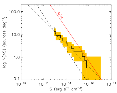
Figure 9.— Cumulative source density versus flux (0.3–8 keV) for only the Galactic sources in our sample. The relations $\log N(>S)\propto S^{\alpha}$ with $\alpha=-1$ (dotted line) and $\alpha=-1.5$ (dashed line, expected slope for an isotropic distribution), each normalized to the faintest flux in our sample, are also included. For comparison, we also show the $\log N-\log S$ curve for AGNs from Kim et al. (2007; solid red line), which indeed has a slope close to $\alpha=-1.5$. Correction for Galactic absorption was done with the model from Drimmel et al. (2003); the model from Schlegel et al. (1998) gives a consistent result. See the electronic edition of the Journal for a color version of this figure.

4.2.3 Source templates

In this study we have avoided the central, most obscured part of the plane, which enabled us to use the properties of the optical and nIR counterparts for source classification. Would Chandra have detected our sources if they were located in the central bulge, and if so, can we use them as templates to constrain the nature of more distant obscured sources? We answer this question for the specific case of the 10′ $\times$ 10′ region around Sgr A*—the Galactic center region or GCR—where Chandra found a large number (thousands) of X-ray point sources, most of which remain unidentified at other wavelengths. We apply the canonical extinction for the GCR of $N_{\rm H,X}=6\times 10^{22}$ cm^-2 to our intrinsic source fluxes, and put them at a distance of 8.5 kpc. The deep pointings of the Sgr A* field reach a sensitivity of at least $5\times 10^{-15}$ erg s^-1 cm^-2 ($S/N\geq 3$ between 2–8 keV for 700 ks of stacked exposures; Hong et al. (2009)). All (candidate) AGNs except CBS 2, the two (likely) Galactic accretion-powered sources CBS 7 and CBS 17, and the RS CVn binary CBS 8 would fall above this X-ray limit. Only two sources would be bright enough in the nIR to be detectable in our GCR $K_{s}$ band observations (Laycock et al., 2005), viz. CBS 8 and CBS 17. With $K_{s}\approx 15$ and 14.1, respectively, they would lie above the confusion limit of $K_{s}=15.4$ in most of the region, and $K_{s}=14.5$ in the most crowded region within 1′ of Sgr A*. With higher-resolution images, obtainable with AO imaging, they would be easily detectable. However, as their spectra do not show strong signatures of activity or accretion (not in the optical, at least), it is difficult to distinguish them from the random coincidences with late-type evolved stars, which abound in the old bulge. While Laycock et al. (2005) showed that at most 10% of the unidentified sources around Sgr A* have such bright counterparts, it is important to recognize that it is not only young wind-fed quiescent Be-HMXBs, which have received much of the focus so far, that contribute to this nIR “bright” population of X-ray sources, but also active binaries of the RS CVn-type and symbiotic binaries.

5. Future work

The present work is limited to a small sample of bright sources, but has uncovered a number of interesting systems that are worth detailed follow-up. Some of it is already underway. Servillat et al. (2011) present the results of an optical/nIR study of CBS 7, and optical spectroscopy to establish the nature of CBS 14 is planned. An extension of this work to the entire ChaMPlane database, which is almost 3 orders of magnitude larger, is guaranteed to find more individual sources of interest. It also allows us to construct deeper $\log N-\log S$ curves in distinct sections of the plane with enough statistics to investigate differences in density and distribution of various types (accreting versus non-accreting) of faint Galactic X-ray sources, and can contribute to our understanding of the composition of the resolved part of the Galactic Ridge. Whereas the present study falls short in the number of sources included, source classification of the larger sample has to be done in a more statistical sense than we were able to do for the bright sources.

References

- Angelini & White (2003) Angelini, L., & White, N. E. 2003, ApJ, 586, L71
- Audard et al. (2007) Audard, M., Osten, R. A., Brown, A., Briggs, K. R., Güdel, M., Hodges-Kluck, E., & Gizis, J. E. 2007, A&A, 471, L63
- Balman et al. (2011) Balman, Ş., Godon, P., Sion, E. M., Ness, J.-U., Schlegel, E., Barrett, P. E., & Szkody, P. 2011, ApJ, 741, 84
- Berger et al. (2010) Berger, E. et al. 2010, ApJ, 709, 332
- Bessel & Brett (1988) Bessel, M. S., & Brett, J. M. 1988, PASP, 100, 1134
- Bessel et al. (1998) Bessel, M. S., Castelli, F., & Plez, B. 1998, A&A, 333, 231
- Bessell (1991) Bessell, M. S. 1991, AJ, 101, 662
- Bhatt et al. (2010) Bhatt, H., Pandey, J. C., Kumar, B., Sagar, R., & Singh, K. P. 2010, New Astronomy, 15, 755
- Cardelli et al. (1989) Cardelli, J. A., Clayton, G. C., & Mathis, J. S. 1989, ApJ, 345, 245
- Cruz et al. (2003) Cruz, K. L., Reid, I. N., Liebert, J., Kirkpatrick, J. D., & Lowrance, P. J. 2003, AJ, 126, 2421
- Dempsey et al. (1993) Dempsey, R. C., Linsky, J. L., Fleming, T. A., & Schmitt, J. H. M. M. 1993, ApJSS, 86, 599
- Dempsey et al. (1997) Dempsey, R. C., Linsky, J. L., Fleming, T. A., & Schmitt, J. H. M. M. 1997, ApJ, 478, 358
- Drimmel et al. (2003) Drimmel, R., Cabrera-Lavers, A., & López-Corredoira, M. 2003, A&A, 409, 205
- Ebisawa et al. (2005) Ebisawa, K. et al. 2005, ApJ, 635, 214
- Elebert et al. (2009) Elebert, P. et al. 2009, MNRAS, 395, 884
- Feigelson et al. (2007) Feigelson, E., Townsley, L., Güdel, M., & Stassun, K. 2007, Protostars and Planets V, 313
- Garmire et al. (2003) Garmire, G. P., Bautz, M. W., Ford, P. G., Nousek, J. A., & Ricker, Jr., G. R. 2003, in Society of Photo-Optical Instrumentation Engineers (SPIE) Conference Series, Vol. 4851, Society of Photo-Optical Instrumentation Engineers (SPIE) Conference Series, ed. J. E. Truemper & H. D. Tananbaum, 28–44
- Gehrels (1986) Gehrels, N. 1986, ApJ, 303, 336
- Grindlay et al. (2005) Grindlay, J. et al. 2005, ApJ, 635, 920
- Güdel (2004) Güdel, M. 2004, A&A Rev., 12, 71
- Güdel & Nazé (2009) Güdel, M., & Nazé, Y. 2009, A&A Rev., 17, 309
- Hands et al. (2004) Hands, A. D. P., Warwick, R. S., Watson, M. G., & Helfand, D. J. 2004, MNRAS, 351, 31
- Heinke et al. (2008) Heinke, C. O., Ruiter, A. J., Muno, M. P., & Belczynski, K. 2008, in American Institute of Physics Conference Series, Vol. 1010, A Population Explosion: The Nature & Evolution of X-ray Binaries in Diverse Environments, ed. R. M. Bandyopadhyay, S. Wachter, D. Gelino, & C. R. Gelino, 136–142
- Henry et al. (2004) Henry, T. J., Subasavage, J. P., Brown, M. A., Beaulieu, T. D., Jao, W., & Hambly, N. C. 2004, AJ, 128, 2460
- Hertz & Grindlay (1984) Hertz, P., & Grindlay, J. E. 1984, ApJ, 278, 137
- Hong et al. (2004) Hong, J., Schlegel, E. M., & Grindlay, J. E. 2004, ApJ, 614, 508
- Hong et al. (2011) Hong, J., van den Berg, M., Grindlay, J. E., Servillat, M., & Zhao, P. 2011, accepted for publication in ApJ (arXiv/1103.2477)
- Hong et al. (2005) Hong, J., van den Berg, M., Schlegel, E., Grindlay, J., Koenig, X., Laycock, S., & Zhao, P. 2005, ApJ, 635, 907
- Hong et al. (2009) Hong, J. S., van den Berg, M., Grindlay, J. E., & Laycock, S. 2009, ApJ, 706, 223
- Hornschemeier et al. (2001) Hornschemeier, A. E. et al. 2001, ApJ, 554, 742
- Huensch et al. (1998) Huensch, M., Schmitt, J. H. M. M., & Voges, W. 1998, A&AS, 132, 155
- Jacoby et al. (1984) Jacoby, G. H., Hunter, D. A., & Christian, C. A. 1984, ApJS, 56, 257
- Johnson (1966) Johnson, H. L. 1966, ARA&A, 4, 193
- Kaaret et al. (2006) Kaaret, P., Corbel, S., Tomsick, J. A., Lazendic, J., Tzioumis, A. K., Butt, Y., & Wijnands, R. 2006, ApJ, 641, 410
- Kennea et al. (2009) Kennea, J. A., Mukai, K., Sokoloski, J. L., Luna, G. J. M., Tueller, J., Markwardt, C. B., & Burrows, D. N. 2009, ApJ, 701, 1992
- Kim et al. (2007) Kim, M., Wilkes, B. J., Kim, D.-W., Green, P. J., Barkhouse, W. A., Lee, M. G., Silverman, J. D., & Tananbaum, H. D. 2007, ApJ, 659, 29
- Koenig et al. (2008) Koenig, X., Grindlay, J. E., van den Berg, M., Laycock, S., Zhao, P., Hong, J., & Schlegel, E. M. 2008, ApJ, 685, 463
- Laycock et al. (2005) Laycock, S., Grindlay, J., van den Berg, M., Zhao, P., Hong, J., Koenig, X., Schlegel, E. M., & Persson, S. E. 2005, ApJL, 634, L53
- Lucas et al. (2008) Lucas, P. W. et al. 2008, MNRAS, 391, 136
- Luna et al. (2010) Luna, G. J. M., Sokoloski, J., Mukai, K., & Nelson, T. 2010, The Astronomer’s Telegram, 3053, 1
- Marshall et al. (2006) Marshall, D. J., Robin, A. C., Reylé, C., Schultheis, M., & Picaud, S. 2006, A&A, 453, 635
- Meyer et al. (1997) Meyer, M. R., Calvet, N., & Hillenbrand, L. A. 1997, AJ, 114, 288
- Monet et al. (1998) Monet, D. et al. 1998, USNO-A2.0 (Flagstaff: US Nav. Obs.)
- Motch et al. (2010) Motch, C. et al. 2010, A&A, 523, A92+
- Muno et al. (2009) Muno, M. P. et al. 2009, ApJS, 181, 110
- Mürset et al. (1997) Mürset, U., Wolff, B., & Jordan, S. 1997, A&A, 319, 201
- Nishiyama et al. (2008) Nishiyama, S., Nagata, T., Tamura, M., Kandori, R., Hatano, H., Sato, S., & Sugitani, K. 2008, ApJ, 680, 1174
- Norton et al. (2008) Norton, A. J., Butters, O. W., Parker, T. L., & Wynn, G. A. 2008, ApJ, 672, 524
- Ostlie & Carroll (2007) Ostlie, D., & Carroll, B. 2007, An introduction to Modern Stellar Astrophysics (second edition) (Pearson Addison-Wesley Publishing Company)
- Penner et al. (2008) Penner, K., van den Berg, M., Hong, J., Laycock, S., Zhao, P., & Grindlay, J. 2008, in Astronomical Society of the Pacific Conference Series, Vol. 393, New Horizons in Astronomy, ed. A. Frebel, J. R. Maund, J. Shen, & M. H. Siegel, 247–+
- Phan-Bao et al. (2008) Phan-Bao, N. et al. 2008, MNRAS, 383, 831
- Popowski et al. (2003) Popowski, P., Cook, K. H., & Becker, A. C. 2003, AJ, 126, 2910
- Predehl & Schmitt (1995) Predehl, P., & Schmitt, J. H. M. M. 1995, A&A, 293, 889
- Protassov et al. (2002) Protassov, R., van Dyk, D. A., Connors, A., Kashyap, V. L., & Siemiginowska, A. 2002, ApJ, 571, 545
- Revnivtsev et al. (2008) Revnivtsev, M., Churazov, E., Sazonov, S., Forman, W., & Jones, C. 2008, A&A, 490, 37
- Revnivtsev et al. (2009) Revnivtsev, M., Sazonov, S., Churazov, E., Forman, W., Vikhlinin, A., & Sunyaev, R. 2009, Nature, 458, 1142
- Robrade et al. (2010) Robrade, J., Poppenhaeger, K., & Schmitt, J. H. M. M. 2010, A&A, 513, A12
- Scargle (1982) Scargle, J. D. 1982, ApJ, 263, 835
- Schlegel et al. (1998) Schlegel, D. J., Finkbeiner, D. P., & Davis, M. 1998, ApJ, 500, 525
- Schmitt & Liefke (2004) Schmitt, J. H. M. M., & Liefke, C. 2004, A&A, 417, 651
- Servillat et al. (2011) Servillat, M., Grindlay, J., van den Berg, M., Hong, J., Zhao, P., & Allen, B. 2011, accepted for publication in ApJ (arXiv/1112.0606)
- Silva & Cornell (1992) Silva, D. R., & Cornell, M. E. 1992, ApJS, 81, 865
- Skrutskie et al. (2006) Skrutskie, M. F. et al. 2006, AJ, 131, 1163
- Stocke et al. (1991) Stocke, J. T., Morris, S. L., Gioia, I. M., Maccacaro, T., Schild, R., Wolter, A., Fleming, T. A., & Henry, J. P. 1991, ApJS, 76, 813
- Sugizaki et al. (2001) Sugizaki, M., Mitsuda, K., Kaneda, H., Matsuzaki, K., Yamauchi, S., & Koyama, K. 2001, ApJS, 134, 77
- Sumi (2004) Sumi, T. 2004, MNRAS, 349, 193
- Torres et al. (2004) Torres, M. A. P., Callanan, P. J., Garcia, M. R., Zhao, P., Laycock, S., & Kong, A. K. H. 2004, ApJ, 612, 1026
- Tozzi et al. (2006) Tozzi, P. et al. 2006, A&A, 451, 457
- Vacca et al. (1996) Vacca, W. D., Garmany, C. D., & Shull, J. M. 1996, ApJ, 460, 914
- van den Berg et al. (2006) van den Berg, M. et al. 2006, ApJL, 647, L135
- van den Berg et al. (2009) van den Berg, M., Hong, J. S., & Grindlay, J. E. 2009, ApJ, 700, 1702
- van den Berg et al. (2004) van den Berg, M., Tagliaferri, G., Belloni, T., & Verbunt, F. 2004, A&A, 418, 509
- Vazquez & Feinstein (1990) Vazquez, R. A., & Feinstein, A. 1990, A&AS, 86, 209
- Walborn (1973) Walborn, N. R. 1973, AJ, 78, 1067
- Watson et al. (2009) Watson, M. G. et al. 2009, A&A, 493, 339
- Zhao et al. (2005) Zhao, P., Grindlay, J., Hong, J., Laycock, S., Koenig, X., Schlegel, E., & van den Berg, M. 2005, ApJS, 161, 429