Hinode/EIS Line Profile Asymmetries and Their Relationship
with the Distribution of SDO/AIA Propagating Coronal Disturbance Velocities

Abstract

Using joint observations from Hinode/EIS and the Atmospheric Imaging Array (AIA) on the Solar Dynamics Observatory (SDO) we explore the asymmetry of coronal EUV line profiles. We find that asymmetries exist in all of the spectral lines studied, and not just the hottest lines as has been recently reported in the literature. Those asymmetries indicate that the velocities of the second emission component are relatively consistent across temperature and consistent with the apparent speed at which material is being inserted from the lower atmosphere that is visible in the SDO/AIA images as propagating coronal disturbances. Further, the observed asymmetries are of similar magnitude (a few percent) and width (determined from the RB analysis) across the temperature space sampled and in the small region studied. Clearly, there are two components of emission in the locations where the asymmetries are identified in the RB analysis, their characteristics are consistent with those determined from the SDO/AIA data. There is no evidence from our analysis that this second component is broader than the main component of the line.

¹High Altitude Observatory, National Center for Atmospheric Research, P.O. Box 3000, Boulder CO 80307, USA

²Lockheed Martin Solar and Astrophysics Laboratory, Palo Alto, CA 94304, USA

1 Introduction

Recently, strong upflows of between 50 and 150 km s^-1 have been observed over a broad range of temperatures spanning the chromosphere, through the transition region, and into the corona (De Pontieu et al. 2011). These flows have been associated with pronounced asymmetries in the blue wing of the spectral line profiles observed and have been proposed as the mechanism by which the corona is filled with hot plasma (De Pontieu et al. 2009; McIntosh & De Pontieu 2009). However, the characteristic behavior of this phenomena is still a topic of some debate (Hara et al. 2008; Bryans et al. 2010; Warren et al. 2011; Peter 2010, among others). While most of the literature can agree that the observations contain more than one emitting component that is not instrumental in origin, a product of spectral blending, or the result of geometric projection effects, the specific details of these components have not been sufficiently consolidated, or explained. Indeed, many of the viewpoints are at significant odds with each other. De Pontieu et al. (2009), and subsequent papers, consider the background dominant emission component to be that of the corona which has low velocities compared to the weak, superimposed second component which occurs at high velocities and does not vary excessively with temperature. Peter (2010) also asserted that the asymmetric profile is composed of two components. However, he suggested that the bulk of the emission originates in a relatively narrow ($\sim$50 km s^-1) unshifted component that is superimposed on a significantly broader (${>}$100 km s^-1) “pedestal” of emission that is shifted only slightly (10–20 km s^-1) to the blue of the main component. This is similar to the concept proposed in Peter (2000, 2001). However, the interpretation of the secondary component has now been shifted towards spicule-like motions and Alfvénic turbulence (Peter 2010). Bryans et al. (2010) found outflows with much higher velocities for the second component of the emission than Peter (2010), stating them to be as high as 200 km s^-1. They also reported (like Warren et al. 2011) that the nature of the second component had a temperature dependence, in which outflows were only observed in hot lines (those formed above the formation temperature of the Fe XII 195Å).

In essence we all have the same objective: determine the model of the emission that is minimally consistent with the observed line profiles, but just how do we achieve that? In this short paper we will take some primitive steps in that direction—using a combination of high signal-to-noise imaging observations from the Atmospheric Imaging Assembly (AIA) on the Solar Dynamics Observatory (SDO) to study the observed propagating coronal disturbances (De Pontieu et al. 2011) in combination with the spectra observed by Hinode/EIS (Culhane et al. 2007) of the same region. The target was NOAA Active Region (AR) 11106 that was just to the south and east of disk center on September 16, 2010. In the following section we provide some brief details of the sequence and identify a small fan region for further study.

Our study combines two different techniques; the first being the RB analysis (De Pontieu et al. 2009) of the line profiles in that region, and the second using an SDO/AIA image time series to track the apparent motion of the propagating coronal disturbances (PCDs) rooted at the base of the asymmetric regions (see, e.g., McIntosh & De Pontieu 2009). We find that asymmetries exist in all clean spectral lines studied, and not just the hottest, though these asymmetries can “hide” in certain spectral windows if the behavior of the local continuum emission is not properly accounted for. Those asymmetries indicate that the velocities of the second emission component are relatively consistent across temperature and consistent with the speed at which material is being inserted from the lower atmosphere (McIntosh & De Pontieu 2009). Further, the asymmetries are of similar magnitude (a few percent) and have an 1/e width (determined from the RB analysis) that are consistent across the lines observed and the region chosen for detailed analysis in this short paper.

Clearly, the data analysis shows that more than one emission component is present in some locations. Understanding the make-up of these line profiles is critical to understanding how mass is cycled from the lower atmosphere into the corona, before cooling and returning some time later. The spectra that we detect encode all of these phases of heating and cooling and, as such, represent the most we can possibly learn about the coronal plasma with current instrumentation. The observations indicate that a more sophisticated approach is needed to analyze these spectral datasets, one which should also be used to re-assess the archived data to identify the sources and signatures of heated mass motion throughout the outer solar atmosphere.

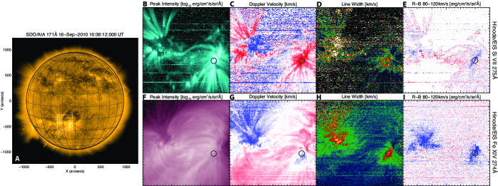
Figure 1.: Contextual imaging and diagnostics of the observed active region. (A) SDO/AIA 171 Å image taken at 10:38:12 UT on September 16, 2010. The white box indicates the observable area analyzed in Hinode/EIS data. (B) and (F) Intensity images from Hinode/EIS. The top row displays Si vii 275 Å and the bottom shows Fe xiv 274 Å. (C) and (G) Doppler Velocities for the active region. (D) and (H) Line profile widths. (E) and (I) RB measurements for each profile, integrated from 80 to 120 km s^-1. The circle indicates the fan under consideration for our detailed analysis, where blue asymmetry is clearly visible.

2 Data and Analysis

The observations we study were taken by the EIS on 10:38:14 UT, September 16, 2010, of NOAA AR 11106. This EIS study (435) was supported as part of HOP 159 by SDO (taking its standard data products at 12 s cadence) and allows us to obtain deep exposures (60 s) of the emission in windows around the Si vii 275 Å, Si x 258 Å and 261 Å, Fe xii 195 Å, Fe xiii 202 Å, Fe xiv 264 Å and 274 Å lines—covering equilibrium formation temperatures from 0.7 MK to 2 MK. The SDO data were recovered from the SDO/JSOC at level 1 having being fully calibrated and corrected. The EIS spectra were prepared using the standard IDL SolarSoft routines distributed by the instrument team. For the purpose of illustration, Fig. 1 shows the field of view of EIS (white rectangle) relative to that of SDO/AIA in panel A.

Single Gaussian fit analysis was performed to each of the EIS spectral windows in turn—the results from the extrema of the temperature range are shown in panels B-D for Si vii 275 Å and F-H for Fe xiv 274 Å. Clearly, there is a stark difference in the emission structure at these temperatures. In addition, we perform an RB line profile asymmetry analysis (De Pontieu et al. 2009) to the data, the results of which are shown in panels E and I integrated from 80–120 km s^-1. Briefly, the RB analysis entails fitting a Gaussian on a linear model background to the line profile to determine line center; interpolating the spectra to 10 times their native resolution; measuring the emission in a narrow (20 km s^-1) range of velocities stepping symmetrically away from the line center once the gradient in the background is removed; the RB measure at the selected velocity is determined as the difference between the emission in the red and blue wings. We note from Fig. 1I that the asymmetries present in the Si vii 275 Å line of this region are weak (see below).

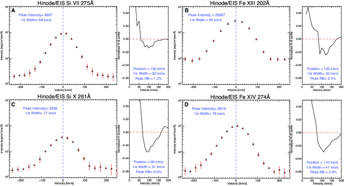
Figure 2.: In pairs these panels show a sample of the EIS line profiles (left) and RB analysis of that profile (right) in the region indicated in Fig. 1 that sample the temperature space. The profiles are fitted with a single Gaussian (and a linear background)—this is needed to determine the centroid of the line that is shown as a blue dashed vertical line. The profiles shown have had the background gradient removed to emphasize the presence of the residual asymmetry. The right panel in each pair shows the peak velocity of the RB second component, the 1/e width of the RB second component, and approximate magnitude of the RB maxima.

After identifying a common region of blue wing asymmetry (the small circled region in Fig. 1) we form an average line profiles (over a $3\times 3$ pixel range) to illustrate behavior over temperature. Those average (background-gradient-removed) line profiles are presented in the left-hand portions of Fig. 2 along with the errors determined in the reduction process (red vertical bars) and the location of the single Gaussian line center fit. For these average profiles (six in total, we show four—one covering each temperature range) we perform the RB analysis and show the results in the right-hand portions of the panels along with the determined properties of the blue second component detected: its central velocity, 1/e width, and magnitude normalized to the single fit peak intensity. We note that in the majority of the analyzed spectra, the background is not a constant across wavelength, but is often tilted (sometimes severely in Si vii 275 Å). We account for this in our analysis by using the linear background fit to estimate the background contribution to the RB measure (in the case of a constant background the RB contribution will be identically zero) such that the real background is subtracted. For the average line profiles there are visible asymmetries in the blue wing—the RB analysis is a means of quantifying the their properties. In all cases, at this location, we see signatures of a second component in the wing that extend from 80 to 150 km s^-1, peaking around 100 km s^-1—consistent with previously published values (e.g., De Pontieu et al. 2009).

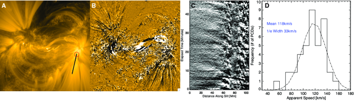
Figure 3.: Studying the propagating coronal disturbances (PCDs) in the fan region. From left to right we show sample AIA 171 Å image, and running difference images, where the former has the location of the “slit” on the fan to study the PCD velocity distribution, the space-time plot determined from the slit location, and the distribution of PCD apparent speeds from sampling five slit angles rooted at the same point. The interested reader can see a movie of panels A and B in an online movie—the link is provided in the text.

One of the goals of this paper is to establish the width of the second component—that causing the blue wing asymmetry. Is it relatively narrow (approximately the same width of the core emission) as the RB analysis will have you believe or is it broad (significantly greater than the core emission) as determined in Peter (2010)? We make the assumption that the second component is not related to the thermal width of the emission and has a strong effect on the non-thermal width—a connection that is visually supported by the RB and line width panels of Figure 1. Also, double Gaussian fits have a very non-linear parameter space (McIntosh et al. 1998) and require a thorough investigation when the sampling of the spectral line is relatively poor—as it is with EIS—so we leave any evaluation that the RB analysis will permit a more strongly constrained double Gaussian fit that is minimally consistent with the data for a future exercise. Instead we look for other avenues of data support in understanding the second emission component. To this end we use the high resolution observations of SDO/AIA to study the distribution of apparent (plane-of-the-sky) speeds seen in the propagating coronal disturbances (PCDs) rooted in the same fan region. McIntosh & De Pontieu (2009) have already demonstrated the common locations and speeds of blue-wing asymmetries and PCDs, here we investigate the PCDs seen to propagate at a small range of angles in the fan and determine the likely distribution of apparent speeds, and hence a possible “width” of the second blue-shifted component. Forming a 100 Mm long slit inclined at an angle of 25^∘ (see Fig. 3) we use space-time plots to characterize the motion of the PCDs as shown in panel C of Fig. 3 and determining the speed using a linear fit to the diagonal intensity signature of the PCD. The distribution of PCD speeds shown in panel D was determined by sampling five space-time plots from slits varying by $\pm 2\hbox{${}^{\circ}$}$ and rooted at the same location in the fan. We see that the mean apparent speed of the PCDs is 118 km s^-1 with a 1/e width of 33 km s^-1.

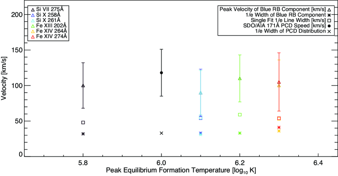
Figure 4.: Information from the line profile and space-time plot analysis of the fan region.

The information from the mean EIS line profiles of the fan root and the study of the PCDs is collated in Figure 4. The triangles show the center position of the blue wing asymmetry with a 1/e width demonstrated as a vertical error bar and pictorially as an asterisk. The latter are for comparison with the single Gaussian fit 1/e width determinations for each line (square symbols). In addition, the PCD values of mean velocity and 1/e width are show for the AIA 171 Å channel as a dot, vertical error-bar, and cross respectively. Summarizing the plot we see little evidence that there is a strong temperature dependence of the RB asymmetry position or width, the former being largely consistent with the AIA determined speeds, with the obvious provision of directly comparing line-of-sight (LOS) and plane-of-sky (POS) speeds. Furthermore, the widths of the RB measure second component ($\sim$35 km s^-1) are systematically smaller than the 1/e width of the single Gaussian fits ($\sim$75 km s^-1) and are commensurate with the width of the PCD speed distribution.

3 Discussion

Based on the evidence presented we can comment on the minimally consistent picture of asymmetries in EIS line profiles observed in portions of an active region:

1. There is (more often than not) more than one (non-blend) component of emission in an EIS resolution element; consider a $\chi^{2}$ map of a single Gaussian fit—does the image contain structure that resembles the peak intensity pattern?

2. There is a preponderance of asymmetry in the blue wing of the emission lines of at the magnetic footpoints of non-flaring active regions—based on the RB analysis of the data considered, that asymmetry is centered at a similar speed, around $\sim$110 km s^-1.

3. The background of the line profiles must be carefully considered and accounted for when quantifying any profile asymmetry.

4. The width of that component giving rise to the blue wing asymmetry is of order 40 km s^-1 while the line widths are of order 70 km s^-1, they are not considerably larger.

5. The properties of the RB analysis determined component is consistent with the properties of the PCDs clearly observed in SDO/AIA image sequences.

These points (the last couple in particular) appear to indicate that the asymmetric line profiles observed by EIS are not always consistent with a very broad weakly shifted “pedestal” component and an unshifted core as presented by Peter (2010) (and Peter 2001). This comes, of course, with the provision that it is very difficult to quantify the degree of Alfvénic transverse motion of the PCDs that can symmetrically broaden this component—a 20 km s^-1 PCD Alfvénic motion (McIntosh et al. 2008a, 2011) would widen that component from 40 to 45 km s^-1 (using a quadratic summation) and not by considerably more. The consistency of the RB peak speed supports recent observations (De Pontieu & McIntosh 2010; Tian et al. 2011) which counter the notion that all PCDs are slow-mode longitudinal waves (e.g., Wang et al. 2009; Verwichte et al. 2010). Further, we note that the asymmetries can be small, very small, and so background emission can mask them or enhance them depending on the direction of the slope—these factors may have played into the blanket determination of Bryans et al. (2010) that asymmetries are not present in cooler lines. Despite the above points, we anticipate that this location may be abnormal, the magnitude of the asymmetries is not uniform from location to location and line to line (see, e.g., the RB maps of Fig. 1), but very detailed analyses are required to unequivocally determine the properties of asymmetries. The asymmetries, as clearly highlighted in the innovative work of Hara et al. (2008), have a center-to-limb dependence that would suggest that the viewing geometry is very important in determining if, when, where, and how much of an asymmetry is observed and its physical origins (Martínez-Sykora et al. 2011). There is also the issue of the apparent red-shift in the single Gaussian fit to the cooler lines (cf. panels C and G of Fig. 1) in places where blue-wing asymmetries exist—an indication that the same magnetic structure has cooling (radiatively losing energy as it falls) and heated upflowing material contributing to the emission. As illustrated by De Pontieu et al. (2009), this is a complicating factor to many conceptual models of the corona (e.g., Warren et al. 2011) and one that will be pursued in due course.

SDO/AIA image sequences provide invaluable contextual information to help diagnose the origins of line profile asymmetries. Because the PCDs are not shifted out of the broad imaging passbands their propagation can be “tracked” along the coronal structure (e.g., McIntosh et al. 2008b). Using this motion tracking algorithm and extrapolations of the photospheric vector magnetograms we hope to infer the correct propagation angle of the PCDs relative to the line of sight. This will allow us to unify the LOS and POS velocity measures and validate the measurements presented. Therefore, in future work we will explore the properties of the PCDs across the same temperature space sampled by this EIS sequence, investigating also the impact of the magnetic field orientation on the magnitude of asymmetry observed. These asymmetries cannot be ignored: they may carry invaluable information about the initial transport of mass into the corona (De Pontieu et al. 2011). As such they must be investigated fully before we begin to apply double Gaussian fitting methods to spectroscopic data in an ad hoc fashion—a warning also carried by Peter (2010).

4 Conclusion

We have performed a detailed analysis of a small fan root using RB analysis of Hinode/EIS spectra and SDO/AIA imaging. We see that, at this location, asymmetries are present in the blue wing of the emission lines observed that are minimally consistent with a picture where there are two components of emission present. The properties of those asymmetries indicate that the velocities of the second emission component are (relatively) consistent across temperature, they are also of similar magnitude and width. Further, the RB-determined asymmetry properties are also consistent with the distribution of apparent speeds measured from the propagating coronal disturbances visible in SDO/AIA image sequences originating at the same location. Based on these points and the limited region studied, we conclude that there is no evidence from our preliminary analysis that this second emission component at the selected location is broader than the main component of the line—such investigations hold vital clues to the origin and mechanism by which material is “pumped” into the corona.

Acknowledgments

The effort was supported by external funds (NNX08AL22G, NNX08AU30G from NASA and ATM-0925177 from the US NSF). NCAR is sponsored by the National Science Foundation.

References

- Bryans et al. (2010) Bryans, P., Young, P. R., & Doschek, G. A. 2010, ApJ, 715, 1012
- Culhane et al. (2007) Culhane, J. L., Harra, L. K., James, A. M., Al-Janabi, K., Bradley, L. J., Chaudry, R. A., Rees, K., Tandy, J. A., Thomas, P., Whillock, M. C. R., Winter, B., Doschek, G. A., Korendyke, C. M., Brown, C. M., Myers, S., Mariska, J., Seely, J., Lang, J., Kent, B. J., Shaughnessy, B. M., Young, P. R., Simnett, G. M., Castelli, C. M., Mahmoud, S., Mapson-Menard, H., Probyn, B. J., Thomas, R. J., Davila, J., Dere, K., Windt, D., Shea, J., Hagood, R., Moye, R., Hara, H., Watanabe, T., Matsuzaki, K., Kosugi, T., Hansteen, V., & Wikstol, Ø. 2007, Solar Phys., 243, 19
- De Pontieu & McIntosh (2010) De Pontieu, B., & McIntosh, S. W. 2010, ApJ, 722, 1013
- De Pontieu et al. (2011) De Pontieu, B., McIntosh, S. W., Carlsson, M., Hansteen, V. H., Tarbell, T. D., Boerner, P., Martínez-Sykora, J., Schrijver, C. J., & Title, A. M. 2011, Science, 331, 55
- De Pontieu et al. (2009) De Pontieu, B., McIntosh, S. W., Hansteen, V. H., & Schrijver, C. J. 2009, ApJ, 701, L1
- Hara et al. (2008) Hara, H., Watanabe, T., Harra, L. K., Culhane, J. L., Young, P. R., Mariska, J. T., & Doschek, G. A. 2008, ApJ, 678, L67
- Martínez-Sykora et al. (2011) Martínez-Sykora, J., De Pontieu, B., Hansteen, V., & McIntosh, S. W. 2011, ApJ, 732, 84
- McIntosh & De Pontieu (2009) McIntosh, S. W., & De Pontieu, B. 2009, ApJ, 706, L80
- McIntosh et al. (2011) McIntosh, S. W., De Pontieu, B., Carlsson, M., Hansteen, V., Boerner, P., & Goossens, M. 2011, Nat, 475, 477
- McIntosh et al. (2008a) McIntosh, S. W., De Pontieu, B., & Tarbell, T. D. 2008a, ApJ, 673, L219
- McIntosh et al. (2008b) McIntosh, S. W., De Pontieu, B., & Tomczyk, S. 2008b, Solar Phys., 252, 321
- McIntosh et al. (1998) McIntosh, S. W., Diver, D. A., Judge, P. G., Charbonneau, P., Ireland, J., & Brown, J. C. 1998, A&AS, 132, 145
- Peter (2000) Peter, H. 2000, A&A, 360, 761
- Peter (2001) — 2001, A&A, 374, 1108
- Peter (2010) — 2010, A&A, 521, A51
- Tian et al. (2011) Tian, H., McIntosh, S. W., & De Pontieu, B. 2011, ApJ, 727, L37
- Verwichte et al. (2010) Verwichte, E., Marsh, M., Foullon, C., Van Doorsselaere, T., De Moortel, I., Hood, A. W., & Nakariakov, V. M. 2010, ApJ, 724, L194
- Wang et al. (2009) Wang, T. J., Ofman, L., & Davila, J. M. 2009, ApJ, 696, 1448
- Warren et al. (2011) Warren, H. P., Ugarte-Urra, I., Young, P. R., & Stenborg, G. 2011, ApJ, 727, 58