Faddeev equation approach for three-cluster nuclear reactions

Abstract

In this lecture we aim to present a formalism based on Faddeev-like equations for describing nuclear three-cluster reactions that include elastic, transfer and breakup channels. Two different techniques based on momentum-space and configuration-space representations are explained in detail. An important new feature of these methods is the possibility to account for the repulsive Coulomb interaction between two of the three clusters in all channels. Comparison with previous calculations based on approximate methods used in nuclear reaction theory is also discussed.

1 Introduction

Nuclear collision experiments, performed at ion accelerators, are a very powerful tool to study nuclear properties at low and intermediate energies. In order to interpret accumulated experimental data appropriate theoretical methods are necessary enabling the simultaneous description of the available elastic, rearrangement and breakup reactions.

Regardless of its importance, the theoretical description of quantum-mechanical collisions turns out to be one of the most complex and slowly advancing problems in theoretical physics. If during the last decade accurate solutions for the nuclear bound state problem became available, full solution of the scattering problem (containing elastic, rearrangement and breakup channels) remains limited to the three-body case.

The main difficulty is related to the fact that, unlike the bound state wave functions, scattering wave functions are not localized. In configuration space one is obliged to solve multidimensional differential equations with extremely complex boundary conditions; by formulating the quantum-mechanical scattering problem in momentum space one has to deal with non-trivial singularities in the kernel of multivariable integral equations.

A rigorous mathematical formulation of the quantum mechanical three-body problem in the framework of non relativistic dynamics has been introduced by Faddeev in the early sixties Fad_60 , in the context of the three-nucleon system with short range interactions. In momentum space these equations might be slightly modified by formulating them in terms of three-particle transition operators that are smoother functions compared to the system wave functions. Such a modification was proposed by Alt, Grassberger, and Sandhas alt:67a (AGS).

Solutions of the AGS equations with short range interactions were readily obtained in the early seventies. As large computers became available progress followed leading, by the end eighties, to fully converged solutions of these equations for neutron-deuteron ($n$-$d$) elastic scattering and breakup using realistic short range nucleon-nucleon ($N$-$N$) interactions. Nevertheless the inclusion of the long range Coulomb force in momentum space calculations of proton-deuteron ($p$-$d$) elastic scattering and breakup with the same numerical reliability as calculations with short range interactions alone, only become possible in the last decade.

Significant progress has been achieved deltuva:05a ; deltuva:05d by developing the screening and renormalization procedure for the Coulomb interaction in momentum space using a smooth but at the same time sufficiently rapid screening. This technique permitted to extend the calculations to the systems of three-particles with arbitrary masses above the breakup threshold deltuva:06b ; deltuva:07d .

However it has taken some time to formulate the appropriate boundary conditions in configuration space for the three-body problem Merkuriev_71 ; Merkuriev_74 ; MGL_76 and even longer to reformulate the original Faddeev equations to allow the incorporation of long-range Coulomb like interactions Merkuriev_80 ; Merkuriev_81 . Rigorous solution of the three-body problem with short range interactions has been achieved just after these theoretical developments, both below and above breakup threshold. On the other hand the numerical solution for the three-body problem including charged particles above the three-particle breakup threshold has been achieved only recently. First it has been done by using approximate Merkuriev boundary conditions in configuration space kievsky:97 . Nevertheless this approach proved to be a rather complex task numerically, remaining unexplored beyond the $p$-$d$ scattering case, but not yet for the $p$-$d$ breakup.

Finally, very recently configuration space method based on complex scaling have been developed and applied for $p$-$d$ scattering lazauskas:11a . This method allows to treat the scattering problem using very simple boundary conditions, equivalent to the ones employed to solve the bound-state problem.

The aim of this lecture is to present these two recently developed techniques, namely the momentum-space method based on screening and renormalization as well as the configuration-space complex scaling method. This lecture is structured as follows: the first part serves to introduce theoretical formalisms for momentum space and configuration space calculations; in the second part we present some selected calculations with an aim to test the performance and validity of the two presented methods.

2 Momentum-space description of three-particle scattering

We describe the scattering process in a system of three-particles interacting via pairwise short-range potentials $v_{\alpha}$, $\alpha=1,2,3$; we use the odd-man-out notation, that is, $v_{1}$ is the potential between particles 2 and 3. In the framework of nonrelativistic quantum mechanics the center-of-mass (c.m.) and the internal motion can be separated by introducing Jacobi momenta

$$\vec{p}_{\alpha} = \frac{m_{\gamma}\vec{k}_{\beta}-m_{\beta}\vec{k}_{\gamma}}{m_{\beta}+m_{\gamma}},$$ (1)

$$\vec{q}_{\alpha} = \frac{m_{\alpha}(\vec{k}_{\beta}+\vec{k}_{\gamma})-(m_{\beta}+m_{\gamma})\vec{k}_{\alpha}}{m_{\alpha}+m_{\beta}+m_{\gamma}},$$ (2)

with ($\alpha\beta\gamma$) being cyclic permutations of (123); $\vec{k}_{\alpha}$ and $m_{\alpha}$ are the individual particle momenta and masses, respectively. The c.m. motion is free and in the following we consider only the internal motion; the corresponding kinetic energy operator is $H_{0}$ while the full Hamiltonian is

$$H=H_{0}+\sum_{\alpha=1}^{3}v_{\alpha}.$$ (3)

2.1 Alt, Grassberger, and Sandhas equations

We consider the particle $\alpha$ scattering from the pair $\alpha$ that is bound with energy $\epsilon_{\alpha}$. The initial channel state $|b_{\alpha}\vec{q}_{\alpha}\rangle$ is the product of the bound state wave function $|b_{\alpha}\rangle$ for the pair $\alpha$ and a plane wave with the relative particle-pair $\alpha$ momentum $\mathbf{q}_{\alpha}$; the dependence on the discrete quantum numbers is suppressed in our notation. $|b_{\alpha}\vec{q}_{\alpha}\rangle$ is the eigenstate of the corresponding channel Hamiltonian $H_{\alpha}=H_{0}+v_{\alpha}$ with the energy eigenvalue $E=\epsilon_{\alpha}+q^{2}_{\alpha}/2M_{\alpha}$ where $M_{\alpha}$ is the particle-pair $\alpha$ reduced mass. The final channel state is the particle-pair state in the same or different configuration $|b_{\beta}\vec{q}_{\beta}\rangle$ in the case of elastic and rearrangement scattering or, in the case of breakup, it is the state of three free particles $|\vec{p}_{\gamma}\vec{q}_{\gamma}\rangle$ with the same energy $E=p_{\gamma}^{2}/2\mu_{\gamma}+q_{\gamma}^{2}/2M_{\gamma}$ and pair $\gamma$ reduced mass $\mu_{\gamma}$; any set of Jacobi momenta can be used equally well for the breakup state.

The stationary scattering states schmid:74a ; gloeckle:83a corresponding to the above channel states are eigenstates of the full Hamiltonian; they are obtained from the channel states using the full resolvent $G=(E+i0-H)^{-1}$, i.e.,

$$|b_{\alpha}\vec{q}_{\alpha}\rangle^{(+)} = i0G|b_{\alpha}\vec{q}_{\alpha}\rangle,$$ (4)

$$|\vec{p}_{\alpha}\vec{q}_{\alpha}\rangle^{(+)} = i0G|\vec{p}_{\alpha}\vec{q}_{\alpha}\rangle.$$ (5)

The full resolvent $G$ may be decomposed into the channel resolvents $G_{\beta}=(E+i0-H_{\beta})^{-1}$ and/or free resolvent $G_{0}=(E+i0-H_{0})^{-1}$ as

$$G=G_{\beta}+G_{\beta}\bar{v}_{\beta}G,$$ (6)

with $\beta=0,1,2,3$ and $\bar{v}_{\beta}=\sum_{\gamma=1}^{3}\bar{\delta}_{\beta\gamma}v_{\gamma}$ where $\bar{\delta}_{\beta\gamma}=1-{\delta}_{\beta\gamma}$. Furthermore, the channel resolvents

$$G_{\beta}=G_{0}+G_{0}T_{\beta}G_{0},$$ (7)

can be related to the corresponding two-particle transition operators

$$T_{\beta}=v_{\beta}+v_{\beta}G_{0}T_{\beta},$$ (8)

embedded into three-particle Hilbert space. Using these definitions Eqs. (4) and (5) can be written as triads of Lippmann-Schwinger equations

$$|b_{\alpha}\vec{q}_{\alpha}\rangle^{(+)} ={} \delta_{\beta\alpha}|b_{\alpha}\vec{q}_{\alpha}\rangle+G_{\beta}\bar{v}_{\beta}|b_{\alpha}\vec{q}_{\alpha}\rangle^{(+)},$$ (9)

$$|\vec{p}_{\alpha}\vec{q}_{\alpha}\rangle^{(+)} ={} (1+G_{0}T_{\beta})|\vec{p}_{\alpha}\vec{q}_{\alpha}\rangle+G_{\beta}\bar{v}_{\beta}|\vec{p}_{\alpha}\vec{q}_{\alpha}\rangle^{(+)},$$ (10)

with $\alpha$ being fixed and $\beta=1,2,3$; they are necessary and sufficient to define the states $|b_{\alpha}\vec{q}_{\alpha}\rangle^{(+)}$ and $|\vec{p}_{\alpha}\vec{q}_{\alpha}\rangle^{(+)}$ uniquely. However, in scattering problems it may be more convenient to work with the multichannel transition operators $U_{\beta\alpha}$ defined such that their on-shell elements yield scattering amplitudes, i.e.,

$$U_{\beta\alpha}|b_{\alpha}\vec{q}_{\alpha}\rangle=\bar{v}_{\beta}|b_{\alpha}\vec{q}_{\alpha}\rangle^{(+)}.$$ (11)

Our calculations are based on the AGS version alt:67a of three-particle scattering theory. In accordance with Eq. (11) it defines the multichannel transition operators $U_{\beta\alpha}$ by the decomposition of the full resolvent $G$ into channel and/or free resolvents as

$$G=\delta_{\beta\alpha}G_{\alpha}+G_{\beta}U_{\beta\alpha}G_{\alpha}.$$ (12)

The multichannel transition operators $U_{\beta\alpha}$ with fixed $\alpha$ and $\beta=1,2,3$ are solutions of three coupled integral equations

$$U_{\beta\alpha}=\bar{\delta}_{\beta\alpha}G_{0}^{-1}+\sum_{\gamma=1}^{3}\bar{\delta}_{\beta\gamma}T_{\gamma}G_{0}U_{\gamma\alpha}.$$ (13)

The transition matrix $U_{0\alpha}$ to final states with three free particles can be obtained from the solutions of Eq. (13) by quadrature, i.e.,

$$U_{0\alpha}=G_{0}^{-1}+\sum_{\gamma=1}^{3}T_{\gamma}G_{0}U_{\gamma\alpha}.$$ (14)

The on-shell matrix elements $\langle b_{\beta}\vec{q}^{\prime}_{\beta}|U_{\beta\alpha}|b_{\alpha}\vec{q}_{\alpha}\rangle$ are amplitudes (up to a factor) for elastic ($\beta=\alpha$) and rearrangement ($\beta\neq\alpha$) scattering. For example, the differential cross section for the $\alpha+(\beta\gamma)\to\beta+(\gamma\alpha)$ reaction in the c.m. system is given by

$$\frac{d\sigma_{\alpha\to\beta}}{d\Omega_{\beta}}=(2\pi)^{4}M_{\alpha}M_{\beta}\frac{q^{\prime}_{\beta}}{q_{\alpha}}|\langle b_{\beta}\vec{q}^{\prime}_{\beta}|U_{\beta\alpha}|b_{\alpha}\vec{q}_{\alpha}\rangle|^{2}.$$ (15)

The cross section for the breakup is determined by the on-shell matrix elements $\langle\vec{p}^{\prime}_{\gamma}\vec{q}^{\prime}_{\gamma}|U_{0\alpha}|b_{\alpha}\vec{q}_{\alpha}\rangle$. Thus, in the AGS framework all elastic, rearrangement, and breakup reactions are calculated on the same footing.

Finally we note that the AGS equations can be extended to include also the three-body forces as done in Ref. deltuva:09e .

2.2 Inclusion of the Coulomb interaction

The Coulomb potential $w_{C}$, due to its long range, does not satisfy the mathematical properties required for the formulation of standard scattering theory as given in the previous subsection for short-range interactions $v_{\alpha}$. However, in nature the Coulomb potential is always screened at large distances. The comparison of the data from typical nuclear physics experiments and theoretical predictions with full Coulomb is meaningful only if the full and screened Coulomb become physically indistinguishable. This was proved in Refs. taylor:74a ; semon:75a where the screening and renormalization method for the scattering of two charged particles was proposed. We base our treatment of the Coulomb interaction on that idea.

Although we use momentum-space framework, we first choose the screened Coulomb potential in configuration-space representation as

$$w_{R}(r)=w_{C}(r)\;e^{-(r/R)^{n}},$$ (16)

and then transform it to momentum-space. Here $R$ is the screening radius and $n$ controls the smoothness of the screening. The standard scattering theory is formally applicable to the screened Coulomb potential $w_{R}$, i.e., the Lippmann-Schwinger equation yields the two-particle transition matrix

$$t_{R}=w_{R}+w_{R}g_{0}t_{R},$$ (17)

where $g_{0}$ is the two-particle free resolvent. It was proven in Ref. taylor:74a that in the limit of infinite screening radius $R$ the on-shell screened Coulomb transition matrix (screened Coulomb scattering amplitude) $\langle\mathbf{p}^{\prime}|t_{R}|\mathbf{p}\rangle$ with $p^{\prime}=p$, renormalized by an infinitely oscillating phase factor $z_{R}^{-1}(p)=e^{2i\phi_{R}(p)}$, approaches the full Coulomb amplitude $\langle\mathbf{p}^{\prime}|t_{C}|\mathbf{p}\rangle$ in general as a distribution. The convergence in the sense of distributions is sufficient for the description of physical observables in a real experiment where the incoming beam is not a plane wave but wave packet and therefore the cross section is determined not directly by the scattering amplitude but by the outgoing wave packet, i.e., by the scattering amplitude averaged over the initial state physical wave packet. In practical calculations alt:02a ; deltuva:05a this averaging is carried out implicitly, replacing the renormalized screened Coulomb amplitude in the $R\to\infty$ limit by the full one, i.e.,

$$\lim_{R\to\infty}z_{R}^{-1}(p)\langle\mathbf{p}^{\prime}|t_{R}|\mathbf{p}\rangle\to\langle\mathbf{p}^{\prime}|t_{C}|\mathbf{p}\rangle.$$ (18)

Since $z_{R}^{-1}(p)$ is only a phase factor, the above relations indeed demonstrate that the physical observables become insensitive to screening provided it takes place at sufficiently large distances $R$ and, in the $R\to\infty$ limit, coincide with the corresponding quantities referring to the full Coulomb. Furthermore, renormalization by $z_{R}^{-\frac{1}{2}}(p_{i})$ in the $R\to\infty$ limit relates also the screened and full Coulomb wave functions gorshkov:61 , i.e.,

$$\lim_{R\to\infty}(1+g_{0}t_{R})|\mathbf{p}\rangle z_{R}^{-\frac{1}{2}}(p)=|\psi_{C}^{(+)}(\mathbf{p})\rangle.$$ (19)

The screening and renormalization method based on the above relations can be extended to more complicated systems, albeit with some limitations. We consider the system of three-particles with charges $z_{\alpha}$ of equal sign interacting via pairwise strong short-range and screened Coulomb potentials $v_{\alpha}+w_{\alpha R}$ with $\alpha$ being 1, 2, or 3. The corresponding two-particle transition matrices are calculated with the full channel interaction

$$T^{(R)}_{\alpha}=(v_{\alpha}+w_{\alpha R})+(v_{\alpha}+w_{\alpha R})G_{0}T^{(R)}_{\alpha},$$ (20)

and the multichannel transition operators $U^{(R)}_{\beta\alpha}$ for elastic and rearrangement scattering are solutions of the AGS equation

$$U^{(R)}_{\beta\alpha}=\bar{\delta}_{\beta\alpha}G_{0}^{-1}+\sum_{\gamma=1}^{3}\bar{\delta}_{\beta\gamma}T^{(R)}_{\gamma}G_{0}U^{(R)}_{\gamma\alpha};$$ (21)

all operators depend parametrically on the Coulomb screening radius $R$.

In order to isolate the screened Coulomb contributions to the transition amplitude that diverge in the infinite $R$ limit we introduce an auxiliary screened Coulomb potential $W^{\mathrm{c\!\>\!.m\!\>\!.}}_{\alpha R}$ between the particle $\alpha$ and the center of mass (c.m.) of the remaining pair. The same screening function has to be used for both Coulomb potentials $w_{\alpha R}$ and $W^{\mathrm{c\!\>\!.m\!\>\!.}}_{\alpha R}$. The corresponding transition matrix

$$T^{\mathrm{c\!\>\!.m\!\>\!.}}_{\alpha R}=W^{\mathrm{c\!\>\!.m\!\>\!.}}_{\alpha R}+W^{\mathrm{c\!\>\!.m\!\>\!.}}_{\alpha R}G^{(R)}_{\alpha}T^{\mathrm{c\!\>\!.m\!\>\!.}}_{\alpha R},$$ (22)

with $G^{(R)}_{\alpha}=(E+i0-H_{0}-v_{\alpha}-w_{\alpha R})^{-1}$ is a two-body-like operator and therefore its on-shell and half-shell behavior in the limit $R\to\infty$ is given by Eqs. (18) and (19). As derived in Ref. deltuva:05a , the three-particle transition operators may be decomposed as

$$U^{(R)}_{\beta\alpha} = \delta_{\beta\alpha}T^{\mathrm{c\!\>\!.m\!\>\!.}}_{\alpha R}+[1+T^{\mathrm{c\!\>\!.m\!\>\!.}}_{\beta R}G^{(R)}_{\beta}]\tilde{U}^{(R)}_{\beta\alpha}[1+G^{(R)}_{\alpha}T^{\mathrm{c\!\>\!.m\!\>\!.}}_{\alpha R}]\quad$$ (23)

$$= \delta_{\beta\alpha}T^{\mathrm{c\!\>\!.m\!\>\!.}}_{\alpha R}+(U^{(R)}_{\beta\alpha}-\delta_{\beta\alpha}T^{\mathrm{c\!\>\!.m\!\>\!.}}_{\alpha R}).$$ (24)

where the auxiliary operator $\tilde{U}^{(R)}_{\beta\alpha}$ is of short range when calculated between on-shell screened Coulomb states. Thus, the three-particle transition operator $U^{(R)}_{\beta\alpha}$ has a long-range part $\delta_{\beta\alpha}T^{\mathrm{c\!\>\!.m\!\>\!.}}_{\alpha R}$ whereas the remainder $U^{(R)}_{\beta\alpha}-\delta_{\beta\alpha}T^{\mathrm{c\!\>\!.m\!\>\!.}}_{\alpha R}$ is a short-range operator that is externally distorted due to the screened Coulomb waves generated by $[1+G^{(R)}_{\alpha}T^{\mathrm{c\!\>\!.m\!\>\!.}}_{\alpha R}]$. On-shell, both parts do not have a proper limit as $R\to\infty$ but the limit exists after renormalization by an appropriate phase factor, yielding the transition amplitude for full Coulomb

$$\langle b_{\beta}\mathbf{q}^{\prime}_{\beta}|U^{(C)}_{\beta\alpha}|b_{\alpha}\mathbf{q}_{\alpha}\rangle=\delta_{\beta\alpha}\langle b_{\alpha}\mathbf{q}^{\prime}_{\beta}|T^{\mathrm{c\!\>\!.m\!\>\!.}}_{\alpha C}|b_{\alpha}\mathbf{q}_{\alpha}\rangle$$

$$+\lim_{R\to\infty}[Z^{-\frac{1}{2}}_{\beta R}(q^{\prime}_{\beta})\langle b_{\beta}\mathbf{q}^{\prime}_{\beta}|(U^{(R)}_{\beta\alpha}-\delta_{\beta\alpha}T^{\mathrm{c\!\>\!.m\!\>\!.}}_{\alpha R})|b_{\alpha}\mathbf{q}_{\alpha}\rangle Z^{-\frac{1}{2}}_{\alpha R}(q_{\alpha})].\quad$$ (25)

The first term on the right-hand side of Eq. (25) is known analytically taylor:74a ; it corresponds to the particle-pair $\alpha$ full Coulomb transition amplitude that results from the implicit renormalization of $T^{\mathrm{c\!\>\!.m\!\>\!.}}_{\alpha R}$ according to Eq. (18). The $R\to\infty$ limit for the remaining part $(U^{(R)}_{\beta\alpha}-\delta_{\beta\alpha}T^{\mathrm{c\!\>\!.m\!\>\!.}}_{\alpha R})$ of the multichannel transition matrix is performed numerically; due to the short-range nature of this term the convergence with the increasing screening radius $R$ is fast and the limit is reached with sufficient accuracy at finite $R$; furthermore, it can be calculated using the partial-wave expansion. We emphasize that Eq. (25) is by no means an approximation since it is based on the obviously exact identity (24) where the $R\to\infty$ limit for each term exists and is calculated separately.

The renormalization factor for $R\to\infty$ is a diverging phase factor

$$Z_{\alpha R}(q_{\alpha})=e^{-2i\Phi_{\alpha R}(q_{\alpha})},$$ (26)

where $\Phi_{\alpha R}(q_{\alpha})$, though independent of the particle-pair relative angular momentum $l_{\alpha}$ in the infinite $R$ limit, may be realized by

$$\Phi_{\alpha R}(q_{\alpha})=\sigma_{l_{\alpha}}^{\alpha}(q_{\alpha})-\eta_{l_{\alpha}R}^{\alpha}(q_{\alpha}),$$ (27)

with the diverging screened Coulomb phase shift $\eta_{l_{\alpha}R}^{\alpha}(q_{\alpha})$ corresponding to standard boundary conditions and the proper Coulomb one $\sigma_{l_{\alpha}}^{\alpha}(q_{\alpha})$ referring to the logarithmically distorted proper Coulomb boundary conditions. For the screened Coulomb potential of Eq. (16) the infinite $R$ limit of $\Phi_{\alpha R}(q_{\alpha})$ is known analytically,

$$\Phi_{\alpha R}(q_{\alpha})=\mathcal{K}_{\alpha}(q_{\alpha})[\ln{(2q_{\alpha}R)}-C/n],$$ (28)

where $C\approx 0.5772156649$ is the Euler number and $\mathcal{K}_{\alpha}(q_{\alpha})=\alpha_{e.m.}z_{\alpha}\sum_{\gamma}\bar{\delta}_{\gamma\alpha}z_{\gamma}M_{\alpha}/q_{\alpha}$ is the Coulomb parameter with $\alpha_{e.m.}\approx 1/137$. The form of the renormalization phase $\Phi_{\alpha R}(q_{\alpha})$ to be used in the actual calculations with finite screening radii $R$ is not unique, but the converged results show independence of the chosen form of $\Phi_{\alpha R}(q_{\alpha})$.

For breakup reactions we follow a similar strategy. However, the proper three-body Coulomb wave function and its relation to the three-body screened Coulomb wave function is, in general, unknown. This prevents the application of the screening and renormalization method to the reactions involving three free charged particles (nucleons or nuclei) in the final state. However, in the system of two charged particles and a neutral one with $z_{\rho}=0$, the final-state Coulomb distortion becomes again a two-body problem with the screened Coulomb transition matrix

$$T_{\rho R}=w_{\rho R}+w_{\rho R}G_{0}T_{\rho R}.$$ (29)

This makes the channel $\rho$, corresponding to the correlated pair of charged particles, the most convenient choice for the description of the final breakup state. As shown in Ref. deltuva:05d , the AGS breakup operator

$$U^{(R)}_{0\alpha}={}G_{0}^{-1}+\sum_{\gamma=1}^{3}T^{(R)}_{\gamma}G_{0}U^{(R)}_{\gamma\alpha},$$ (30)

can be decomposed as

$$U^{(R)}_{0\alpha}={}(1+T_{\rho R}G_{0})\tilde{U}^{(R)}_{0\alpha}(1+G^{(R)}_{\alpha}T^{\mathrm{c\!\>\!.m\!\>\!.}}_{\alpha R}),$$ (31)

where the reduced operator $\tilde{U}^{(R)}_{0\alpha}(Z)$ calculated between screened Coulomb distorted initial and final states is of finite range. In the full breakup operator $U^{(R)}_{0\alpha}(Z)$ the external distortions show up in screened Coulomb waves generated by $(1+G^{(R)}_{\alpha}T^{\mathrm{c\!\>\!.m\!\>\!.}}_{\alpha R})$ in the initial state and by $(1+T_{\rho R}G_{0})$ in the final state; both wave functions do not have proper limits as $R\to\infty$. Therefore the full breakup transition amplitude in the case of the unscreened Coulomb potential is obtained via the renormalization of the on-shell breakup transition matrix $U^{(R)}_{0\alpha}$ in the infinite $R$ limit

$$\langle\mathbf{p}^{\prime}_{\rho}\mathbf{q}^{\prime}_{\rho}|U^{(C)}_{0\alpha}|b_{\alpha}\mathbf{q}_{\alpha}\rangle=\lim_{R\to\infty}[z^{-\frac{1}{2}}_{\rho R}(p^{\prime}_{\rho})\langle\mathbf{p}^{\prime}_{\rho}\mathbf{q}^{\prime}_{\rho}|U^{(R)}_{0\alpha}|b_{\alpha}\mathbf{q}_{\alpha}\rangle Z_{\alpha R}^{-\frac{1}{2}}(q_{\alpha})],$$ (32)

where $\mathbf{p}^{\prime}_{\rho}$ is the relative momentum between the charged particles in the final state, $\mathbf{q}^{\prime}_{\rho}$ the corresponding particle-pair relative momentum, and

$$z_{\rho R}(p^{\prime}_{\rho})=e^{-2i\kappa_{\rho}(p^{\prime}_{\rho})[\ln{(2p^{\prime}_{\rho}R)}-C/n]},$$ (33)

the final-state renormalization factor with the Coulomb parameter $\kappa_{\rho}(p^{\prime}_{\rho})$ for the pair $\rho$. The limit in Eq. (32) has to be performed numerically, but, due to the short-range nature of the breakup operator, the convergence with increasing screening radius $R$ is fast and the limit is reached with sufficient accuracy at finite $R$. Thus, to include the Coulomb interaction via the screening and renormalization method one only needs to solve standard scattering theory equations.

2.3 Practical realization

We calculate the short-range part of the elastic, rearrangement, and breakup scattering amplitudes (25) and (32) by solving standard scattering equations (21), (22), and (30) with a finite Coulomb screening radius $R$. We work in the momentum-space partial-wave basis deltuva:phd , i.e., we use three sets
$|p_{\alpha}q_{\alpha}\nu_{\alpha}\rangle\equiv|p_{\alpha}q_{\alpha}(l_{\alpha}\{[L_{\alpha}(s_{\beta}s_{\gamma})S_{\alpha}]I_{\alpha}s_{\alpha}\}K_{\alpha}){JM}\rangle$ with $(\alpha,\beta,\gamma)$ being cyclic permutations of (1,2,3). Here $s_{\alpha}$ is the spin of particle $\alpha$, $L_{\alpha}$ and $l_{\alpha}$ are the orbital angular momenta associated with $p_{\alpha}$ and $q_{\alpha}$ respectively, whereas $S_{\alpha}$, $I_{\alpha}$, and $K_{\alpha}$ are intermediate angular momenta that are coupled to a total angular momentum $J$ with projection $M$. All discrete quantum numbers are abbreviated by $\nu_{\alpha}$. The integration over the momentum variables is discretized using Gaussian quadrature rules thereby converting a system of integral equations for each $J$ and parity $\Pi=(-)^{L_{\alpha}+l_{\alpha}}$ into a very large system of linear algebraic equations. Due to the huge dimension those linear systems cannot be solved directly. Instead we expand the AGS transition operators (21) into the corresponding Neumann series

$$U^{(R)}_{\beta\alpha}=\bar{\delta}_{\beta\alpha}G_{0}^{-1}+\sum_{\gamma=1}^{3}\bar{\delta}_{\beta\gamma}T^{(R)}_{\gamma}\bar{\delta}_{\gamma\alpha}+\sum_{\gamma=1}^{3}\bar{\delta}_{\beta\gamma}T^{(R)}_{\gamma}G_{0}\sum_{\sigma=1}^{3}\bar{\delta}_{\gamma\sigma}T^{(R)}_{\sigma}\bar{\delta}_{\sigma\alpha}+\cdots,$$ (34)

that are summed up by the iterative Pade method chmielewski:03a ; it yields an accurate solution of Eq. (21) even when the Neumann series (34) diverges. Each two-particle transition operator $T^{(R)}_{\gamma}$ is evaluated in its proper basis $|p_{\gamma}q_{\gamma}\nu_{\gamma}\rangle$, thus, transformations between all three bases are needed. The calculation of the involved overlap functions $\langle p_{\beta}q_{\beta}\nu_{\beta}|p_{\alpha}q_{\alpha}\nu_{\alpha}\rangle$ follows closely the calculation of three-nucleon permutation operators discussed in Refs. deltuva:phd ; gloeckle:83a . A special treatment chmielewski:03a ; deltuva:phd is needed for the integrable singularities arising from the pair bound state poles in $T^{(R)}_{\gamma}$ and from $G_{0}$. Furthermore, we have to make sure that $R$ is large enough to achieve (after renormalization) the $R$-independence of the results up to a desired accuracy. However, those $R$ values are larger than the range of the nuclear interaction resulting in a slower convergence of the partial-wave expansion. As we found in Ref. deltuva:05a , the practical success of the screening and renormalization method depends very much on the choice of the screening function, in our case on the power $n$ in Eq. (16). We want to ensure that the screened Coulomb potential $w_{R}$ approximates well the true Coulomb one $w_{C}$ for distances $r<R$ and simultaneously vanishes rapidly for $r>R$, providing a comparatively fast convergence of the partial-wave expansion. As shown in Ref. deltuva:05a , this is not the case for simple exponential screening $(n=1)$ whereas the sharp cutoff $(n\to\infty)$ yields slow oscillating convergence with the screening radius $R$. However, we found that values of $3\leq n\leq 8$ provide a sufficiently smooth and rapid screening around $r=R$. The screening functions for different $n$ values are compared in Ref. deltuva:05a together with the results demonstrating the superiority of our optimal choice: using $3\leq n\leq 8$ the convergence with the screening radius $R$, at which the short range part of the amplitudes was calculated, is fast enough such that the convergence of the partial-wave expansion, though being slower than for the nuclear interaction alone, can be achieved and there is no need to work in a plane-wave basis. Here we use $n=4$ and show in Figs. 1and 2 few examples for the $R$-convergence of the $\alpha$-deuteron scattering observables calculated in a three-body model $(\alpha,p,n)$; the nuclear interaction is taken from Ref. deltuva:06b . The convergence with $R$ is impressively fast for both $\alpha$-deuteron elastic scattering and breakup. In addition we note that the Coulomb effect is very large and clearly improves the description of the experimental data, especially for the differential cross section in $\alpha$-deuteron breakup reaction. This is due to the shift of the $\alpha p$ $P$-wave resonance position when the $\alpha p$ Coulomb repulsion is included that leads to the corresponding changes in the structure of the observables.

t]

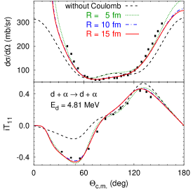
Figure 1: Differential cross section and deuteron vector analyzing power $iT_{11}$ of the $\alpha d$ elastic scattering at 4.81 MeV deuteron lab energy as functions of the c.m. scattering angle. Convergence with the screening radius $R$ used to calculate the short-range part of the amplitudes is studied: $R=5$ fm (dotted curves), $R=10$ fm (dash-dotted curves), and $R=15$ fm (solid curves). Results without Coulomb are given by dashed curves. The experimental data are from Refs. bruno:80 ; gruebler:70a .

t]

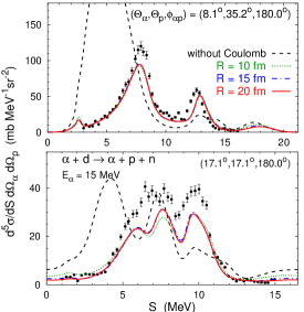
Figure 2: Fivefold differential cross section of the $\alpha d$ breakup reaction at 15 MeV $\alpha$ lab energy for several combinations of $\alpha$ and proton scattering angles as function of the final-state energy variable $S$ with $dS=(dE_{\alpha}^{2}+dE_{p}^{2})^{1/2}$. Convergence with the screening radius $R$ is studied: $R=10$ fm (dotted curves), $R=15$ fm (dash-dotted curves), and $R=20$ fm (solid curves). Results without Coulomb are given by dashed curves. The experimental data are from Ref. koersner:77 .

In addition to the internal reliability criterion of the screening and renormalization method — the convergence with $R$ — we note that our results for proton-deuteron elastic scattering deltuva:05b agree well over a broad energy range with those of Ref. kievsky:01a obtained from the variational configuration-space solution of the three-nucleon Schrödinger equation with unscreened Coulomb potential and imposing the proper Coulomb boundary conditions explicitly.

3 Configuration space

In contrast to the momentum-space representation, the Coulomb interaction has a trivial expression in configuration space and thus may seem to be easier to handle. However the major obstacle for configuration-space treatment of the scattering problem is related with the complexity of the wave function asymptotic structure, which strongly complicates once three-particle breakup is available. Although for short range interactions the analytical behavior of the breakup asymptote of the configuration space wave function is well established, this is not a case once long range interactions (like Coulomb) are present. Therefore a method which enables the scattering problem to be solved without explicit use of the wave function asymptotic form is of great importance. The complex scaling method has been proposed Nuttal_csm ; CSM_71 and successfully applied to calculate the resonance positions Moiseyev by using bound state boundary conditions. As has been demonstrated recently this method can be extended also for the scattering problem CSM_Curdy_04 ; Elander_CSM . We demonstrate here that this method may be also successfully applied to solve three-particle scattering problems which include the long-range Coulomb interaction together with short range optical potentials.

3.1 Faddeev-Merkuriev equations

Like in the momentum space formalism described above Jacobi coordinates are also used in configuration space to separate the center of mass of the three-particle system. One has three equivalent sets of three-particle Jacobi coordinates

$$\mathbf{x}_{\alpha} = \sqrt{\frac{2m_{\beta}m_{\gamma}}{(m_{\beta}+m_{\gamma})m}}(\mathbf{r}_{\gamma}-\mathbf{r}_{\beta}),$$ (35)

$$\mathbf{y}_{\alpha} = \sqrt{\frac{2m_{\beta}(m_{\beta}+m_{\gamma})}{(m_{\alpha}+m_{\beta}+m_{\gamma})m}}(\mathbf{r}_{\alpha}-\frac{m_{\beta}\mathbf{r}_{\beta}+m_{\gamma}\mathbf{r}_{\gamma}}{m_{\beta}+m_{\gamma}}),$$

here $r_{\alpha}$ and $m_{\alpha}$ are individual particle position vectors and masses, respectively. The choice of a mass scale $m$ is arbitrary. The three-particle problem is formulated here using Faddeev-Merkuriev (FM) equations Merkuriev_80 :

$$(E-H_{0}-\sum_{\kappa=1}^{3}w_{i}^{l})\psi_{\alpha}=(v_{\alpha}+w_{\alpha}^{s})(\psi_{\alpha}+\psi_{\beta}+\psi_{\gamma}),$$

$$(E-H_{0}-\sum_{\kappa=1}^{3}w_{i}^{l})\psi_{\beta}=(v_{\beta}+w_{\beta}^{s})(\psi_{\alpha}+\psi_{\beta}+\psi_{\gamma}),$$ (36)

$$(E-H_{0}-\sum_{\kappa=1}^{3}w_{i}^{l})\psi_{\gamma}=(v_{\gamma}+w_{\gamma}^{s})(\psi_{\alpha}+\psi_{\beta}+\psi_{\gamma}),$$

where the Coulomb interaction is split in two parts (short and long range), $w_{\alpha}=w_{\alpha}^{s}+w_{\alpha}^{l}$, by means of some arbitrary cut-off function $\chi_{\alpha}(x_{\alpha},y_{\alpha})$:

$$w_{\alpha}^{s}(x_{\alpha},y_{\alpha})=w_{\alpha}(x_{\alpha})\chi_{\alpha}(x_{\alpha},y_{\alpha})\qquad w_{\alpha}^{l}(x_{\alpha},y_{\alpha})=w_{\alpha}(x_{\alpha})[1-\chi_{\alpha}(x_{\alpha},y_{\alpha})]$$ (37)

This cut-off function intends to shift the full Coulomb interaction in the $w_{\alpha}^{s}$ term if $x_{\alpha}$ is small, whereas the $w_{\alpha}^{l}$ term acquires the full Coulomb interaction if $x_{\alpha}$ becomes large and $y_{\alpha}<x_{\alpha}$. The practical choice of function $\chi_{\alpha}(x_{\alpha},y_{\alpha})$ has been proposed in Merkuriev_80 :

$$\chi_{\alpha}(x_{\alpha},y_{\alpha})=\frac{2}{[1+exp{(\frac{[x_{\alpha}/x_{0}]^{\mu}}{1+y_{\alpha}/y_{0}})}]},$$ (38)

with free parameters $x_{0},y_{0}$ having size comparable with the charge radii of the respective binary systems; the value of parameter $\mu$ must be larger than 1 and is usually set $\mu\approx 2$. In such a way the so-called Faddeev amplitude $\psi_{\alpha}$ intends to acquire full asymptotic behavior of the binary $\alpha-(\beta\gamma)$ channels, i.e:

$$\psi_{\alpha}(\mathbf{x}_{\alpha},\mathbf{y}_{\alpha}\rightarrow\infty)=\delta_{\kappa,\alpha}\psi_{\alpha}^{i_{\kappa}}(\mathbf{x}_{\alpha})\phi_{\alpha}^{i_{\kappa},in}(\mathbf{y}_{\alpha}) + \sum_{j_{\alpha}}f_{j_{\alpha i_{\kappa}}}(\mathbf{x}_{\alpha}.\mathbf{y}_{\alpha})\psi_{\alpha}^{j_{\alpha}}(\mathbf{x}_{\alpha})\phi_{\alpha}^{j_{\alpha},out}(\mathbf{y}_{\alpha})$$ (39)

$$+ A_{i_{\kappa}}(\mathbf{x}_{\alpha},\mathbf{y}_{\alpha})\Phi_{i_{\kappa}}^{out}(\mathbf{\rho}),$$

where the hyperradius is $\rho=\sqrt{x_{\alpha}^{2}+y_{\alpha}^{2}}$. An expression $\varphi_{\alpha}^{i_{\alpha}}(\mathbf{x}_{\alpha})\phi_{\alpha}^{i_{\kappa},in}(\mathbf{y}_{\alpha})$ represents the incoming wave for particle $\alpha$ on pair $(\beta\gamma)$ in the bound state $i_{\alpha}$, with $\varphi_{\alpha}^{i_{\alpha}}(\mathbf{x}_{\alpha})$ representing the normalized wave function of bound state $i_{\alpha}$. This wave function is a solution of the $(E-H_{0}-w_{\alpha}-v_{\alpha}-W_{\alpha}^{c.m.})$ two-body Hamiltonian. The $\phi_{\alpha}^{j_{\alpha},out}(\mathbf{y}_{\alpha})$ and $\Phi_{i_{\kappa}}^{out}(\mathbf{\rho}_{\alpha})$ represent outgoing waves for binary and three-particle breakup channels respectively. In the asymptote, one has the following behavior:

$$\varphi_{\alpha}^{i_{\alpha}}(x_{\alpha} \rightarrow \infty)\propto\exp(-k_{i_{\alpha}}x_{\alpha}),$$

$$\phi_{\alpha}^{i_{\alpha},out}(y_{\alpha} \rightarrow \infty)\propto\exp(iq_{i_{\alpha}}y_{\alpha}),$$ (40)

$$\Phi_{i_{\alpha}}^{out}(\rho \rightarrow \infty)\propto\exp(iK\rho),$$ (41)

with $k_{i_{\alpha}}=\sqrt{-\varepsilon_{{}_{i_{\alpha}}}m}$ representing momentum of 2-body bound state $i_{\alpha}$ with a negative binding energy $\varepsilon_{{}_{i_{\alpha}}}$; $q_{i_{\alpha}}=\sqrt{(E-\varepsilon_{{}_{i_{\alpha}}})m}$ is relative scattering momentum for the $\alpha-(\beta\gamma)$ binary channel, whereas $K=\sqrt{mE}$ is a three-particle breakup momentum (three-particle breakup is possible only if energy value $E$ is positive).

When considering particle’s $\alpha$ scattering on the bound state $i_{\alpha}$ of the pair $(\beta\gamma)$, it is convenient to separate readily incoming wave $\psi_{\alpha}^{i_{\alpha},in}=\psi_{\alpha}^{i_{\alpha}}(\mathbf{x}_{\alpha})\phi_{\alpha}^{i_{\alpha},in}(\mathbf{y}_{\alpha})$, by introducing:

$$\psi_{\alpha}^{i_{\alpha},out} = \psi_{\alpha}^{i_{\alpha}}-\psi_{\alpha}^{i_{\alpha}}(\mathbf{x}_{\alpha})\phi_{\alpha}^{i_{\alpha},in}(\mathbf{y}_{\alpha}),$$ (42)

$$\psi_{\beta}^{i_{\alpha},out} = \psi_{\beta}^{i_{\alpha}}\qquad\beta\neq\alpha,$$

Then Faddeev-Merkuriev equations might be rewritten in a so-called driven form:

$$(E-H_{0}-\sum_{\kappa=1}^{3}w_{\kappa}^{l})\psi_{\alpha}^{out} = (v_{\alpha}+w_{\alpha}^{s})(\psi_{\alpha}^{out}+\psi_{\beta}^{out}+\psi_{\gamma}^{out})+\left[\sum_{\kappa=1}^{3}w_{\kappa}^{l}-w_{\alpha}-W_{\alpha}^{c.m.}\right]\psi_{\alpha}^{in},$$

$$(E-H_{0}-\sum_{\kappa=1}^{3}w_{\kappa}^{l})\psi_{\beta}^{out} = (v_{\beta}+w_{\beta}^{s})(\psi_{\alpha}^{out}+\psi_{\beta}^{out}+\psi_{\gamma}^{out}+\psi_{\alpha}^{in}),$$ (43)

$$(E-H_{0}-\sum_{\kappa=1}^{3}w_{\kappa}^{l})\psi_{\gamma}^{out} = (v_{\gamma}+w_{\gamma}^{s})(\psi_{\alpha}^{out}+\psi_{\beta}^{out}+\psi_{\gamma}^{out}+\psi_{\alpha}^{in}).$$

In this expression index of the incoming state $i_{\alpha}$ has been omitted in all Faddeev component expressions $\psi_{\alpha}^{in}$ and $\psi_{\alpha}^{out}$.

3.2 Complex scaling

Next step is to perform the complex scaling operations i.e. scale all the distances $x$ and $y$ by a constant complex factor $e^{i\theta},$ so that both $Re(e^{i\theta})$ and $Im(e^{i\theta})$ are positive (angle $\theta$ must be chosen in the first quartet in order to satisfy this condition). The complex scaling operation, in particular, implies that the analytical continuation of the interaction potentials is performed: $v_{\alpha}(x_{\alpha}e^{i\theta})$ and $w_{\alpha}(x_{\alpha}e^{i\theta})$. Therefore the complex scaling method may be used only if these potentials are analytic. It is easy to see that the solutions of the complex scaled equations coincide with the ones obtained without complex scaling but to which the complex scaling operation is applied: $\left[\psi(x_{\alpha},y_{\alpha})\right]^{CS}=\psi(x_{\alpha}e^{i\theta},y_{\alpha}e^{i\theta})$.

Namely, it is easy to demonstrate that all the outgoing wave functions of eq.(41) becomes exponentially bound after the complex scaling operation:

$$\left[\varphi_{\alpha}^{i_{\alpha}}(x_{\alpha}\rightarrow\infty)\right]^{CS} \propto \exp(-k_{i_{\alpha}}x_{\alpha}\cos\theta),$$

$$\left[\phi_{\alpha}^{i_{\alpha},out}(y_{\alpha}\rightarrow\infty)\right]^{CS} \propto \exp(-q_{i_{\alpha}}y_{\alpha}\sin\theta),$$ (44)

$$\left[\Phi_{i_{\alpha}}^{out}(\rho\rightarrow\infty)\right]^{CS} \propto \exp(-K\rho\sin\theta).$$

Nevertheless an incoming wave diverges in $y_{\alpha}$ after the complex scaling:

$$\left[\phi_{\alpha}^{i_{\alpha},out}(y_{\alpha}\rightarrow\infty)\right]^{CS}\propto\exp(+q_{i_{\alpha}}y_{\alpha}\sin\theta).$$ (45)

However these terms appear only on the right hand sides of the driven Faddeev-Merkuriev equation (3.1) being pre-multiplied with the potential terms and under certain conditions they may vanish outside of some finite (resolution) domain $x_{\alpha}\in[0,x^{\max}]$ and $y_{\alpha}\in[0,y^{\max}]$. Let us consider the long range behavior of the term $\left[(v_{\beta}+w_{\beta}^{s})\psi_{\alpha}^{in}\right]^{CS}$. Since the interaction terms $v_{\beta}$ and $w_{\beta}^{s}$ are of short range, the only region the former term might not converge is along $y_{\beta}$ axis in $(x_{\beta},y_{\beta})$ plane, i.e. for $x_{\beta}\ll y_{\beta}$. On the other hand $x_{\alpha}(\mathbf{x}_{\beta}\mathbf{,y}_{\beta})\approx\sqrt{m_{\gamma}/(m_{\gamma}+m_{\beta})}\sqrt{M/(m_{\gamma}+m_{\alpha})}y_{\beta}$ and $y_{\alpha}(\mathbf{x}_{\beta}\mathbf{,y}_{\beta})\approx\sqrt{m_{\beta}/(m_{\gamma}+m_{\beta})}\sqrt{m_{\alpha}/(m_{\gamma}+m_{\alpha})}y_{\beta}$ under condition $x_{\beta}\ll y_{\beta}$. Then one has:

$$\small{\left[(v_{\beta}+w_{\beta}^{s})\psi_{\alpha}^{i_{\alpha},in}\right]^{CS}_{x_{\beta}\ll y_{\beta}}\propto\exp\left(-k_{i_{\alpha}}\sqrt{\frac{m_{\gamma}M}{(m_{\gamma}+m_{\beta})(m_{\gamma}+m_{\alpha})}}y_{\beta}\cos\theta+q_{i_{\alpha}}\sqrt{\frac{m_{\alpha}m_{\beta}}{(m_{\gamma}+m_{\beta})(m_{\gamma}+m_{\alpha})}}y_{\beta}\sin\theta\right)}.$$ (46)

This term becomes bound to finite domain in $(x_{\beta},y_{\beta})$ plane, if condition:

$$\tan\theta<\sqrt{\frac{m_{\gamma}M}{m_{\alpha}m_{\beta}}}\frac{k_{i_{\alpha}}}{q_{i_{\alpha}}}=\sqrt{\frac{m_{\gamma}M}{m_{\alpha}m_{\beta}}}\sqrt{\frac{\left|B_{{}_{i_{\alpha}}}\right|}{E+\left|B_{{}_{i_{\alpha}}}\right|}},$$ (47)

is satisfied. This implies that for rather large scattering energies $E$, above the break-up threshold, one is obliged to use rather small complex scaling parameter $\theta$ values.

The term $\left[\sum_{\kappa=1}^{3}w_{\kappa}^{l}-w_{\alpha}-W_{\alpha}^{c.m.}\right]\psi_{\alpha}^{i_{\alpha},in}$, in principle, is not exponentially bound after the complex scaling. It represents the higher order corrections to the residual Coulomb interaction between particle $\alpha$ and bound pair $(\beta\gamma)$. These corrections are weak $o(1/y^{2})$ and might be neglected by suppressing this term close to the border of the resolution domain. Alternative possibility might be to use incoming wave functions, which account not only for the bare $\alpha-(\beta\gamma)$ Coulomb interaction but also takes into account higher order polarization corrections.

Extraction of the scattering observables is realized by employing Greens theorem. One might demonstrate that strong interaction amplitude for $\alpha-(\beta\gamma)$ collision is:

$$f_{j_{\alpha i_{\kappa}}}(\mathbf{x}_{\alpha}.\mathbf{y}_{\alpha})=-\frac{m}{q_{j_{\alpha}}}\int\int\left[(\psi_{\alpha}^{j_{\alpha},in})^{*}\right]^{CS}(\overline{v}_{\alpha}+\overline{w}_{\alpha}-W_{\alpha}^{c.m.})^{CS}\left[\Psi_{i_{\kappa}}\right]^{CS}e^{6i\theta}d^{3}\mathbf{x}_{i}d^{3}\mathbf{y}_{i},$$ (48)

with $\left[\Psi_{i_{\kappa}}\right]^{CS}=\left[\psi_{\alpha}^{i_{\kappa},out}+\psi_{\beta}^{i_{\kappa},out}+\psi_{\gamma}^{i_{\kappa},out}+\psi_{\alpha}^{i_{\kappa},in}\right]^{CS}$ being the total wave function of the three-body system. In the last expression the term containing product of two incoming waves is slowest to converge. Even stronger constraint than eq.(47) should be implied on complex scaling angle in order to make this term integrable on the finite domain. Nevertheless this term contains only the product of two-body wave functions and might be evaluated without using complex scaling prior to three-body solution. Then the appropriate form of the integral (48) to be used becomes:

$$f_{j_{\alpha i_{\kappa}}}(\mathbf{x}_{\alpha}.\mathbf{y}_{\alpha}) = -\frac{m}{q_{j_{\alpha}}}\int\int\left[(\psi_{\alpha}^{j_{\alpha},in})^{*}\right]^{CS}(\overline{v}_{\alpha}+\overline{w}_{\alpha}-W_{\alpha}^{c.m.})^{CS}\left[\Psi_{i_{\kappa}}-\psi_{\alpha}^{j_{\alpha},in}\right]^{CS}e^{6i\theta}d^{3}\mathbf{x}_{i}d^{3}\mathbf{y}_{i}$$ (49)

$$-\frac{m}{q_{j_{\alpha}}}\int\int(\psi_{\alpha}^{j_{\alpha},in})^{*}(\overline{v}_{\alpha}+\overline{w}_{\alpha}-W_{\alpha}^{c.m.})\psi_{\alpha}^{j_{\alpha},in}d^{3}\mathbf{x}_{i}d^{3}\mathbf{y}.$$

4 Application to three-body nuclear reactions

The two methods presented in sections 2 and 3 were first applied to the proton-deuteron elastic scattering and breakup deltuva:05a ; deltuva:05d ; deltuva:09e ; lazauskas:11a . The three-nucleon system is the only nuclear three-particle system that may be considered realistic in the sense that the interactions are given by high precision potentials valid over a broad energy range. Nevertheless, in the same way one considers the nucleon as a single particle by neglecting its inner quark structure, in a further approximation one can consider a cluster of nucleons (composite nucleus) to be a single particle that interacts with other nucleons or nuclei via effective potentials whose parameters are determined from the two-body data. A classical example is the $\alpha$ particle, a tightly bound four-nucleon cluster. As shown in Figs. 1 and 2 and in Ref. deltuva:06b , the description of the $(\alpha,p,n)$ three-particle system with real potentials is quite successful at low energies but becomes less reliable with increasing energy where the inner structure of the $\alpha$ particle cannot be neglected anymore. At higher energies the nucleon-nucleus or nucleus-nucleus interactions are modeled by optical potentials (OP) that provide quite an accurate description of the considered two-body system in a given narrow energy range; these potentials are complex to account for the inelastic excitations not explicitly included in the model space. The methods based on Faddeev/AGS equations can be applied also in this case, however, the potentials within the pairs that are bound in the initial or final channel must remain real. The comparison of the two methods based on the AGS and FM equations will be performed in section 4.1 for such an interaction model with OP.

In the past the description of three-body-like nuclear reactions involved a number of approximate methods that have been developed. Well-known examples are the distorted-wave Born approximation (DWBA), various adiabatic approaches johnson:70a , and continuum-discretized coupled-channels (CDCC) method austern:87 . Compared to them the present methods based on exact Faddeev or AGS equations, being more technically and numerically involved, have some disadvantages. Namely, their application in the present technical realization is so far limited to a system made of two nucleons and one heavier cluster. The reason is that the interaction between two heavier cluster involves very many angular momentum states and the partial-wave convergence cannot be achieved. The comparison between traditional nuclear reaction approaches and momentum-space Faddeev/AGS methods for various neutron + proton + nucleus systems are summarized in section 4.2.

On the other hand, the Faddeev and AGS methods may be more flexible with respect to dynamic input and thereby allows to test novel aspects of the nuclear interaction not accessible with the traditional approaches. Few examples will be presented in section 4.3.

4.1 Numerical comparison of AGS and FM methods

As an example we consider the $n+p+^{12}C$ system. For the $n$-$p$ interaction we use a realistic AV18 model wiringa:95a that accurately reproduces the available two-nucleon scattering data and deuteron binding energy. To study not only the $d+{}^{12}$C but also $p+{}^{13}$C scattering and transfer reactions we use a $n$-¹²C potential that is real in the ${}^{2}P_{\frac{1}{2}}$ partial wave and supports the ground state of ${}^{13}C$ with 4.946 MeV binding energy; the parameters are taken from Ref. nunes:11b . In all other partial waves we use the $n$-¹²C optical potential from Ref. CH89 taken at half the deuteron energy in the $d+{}^{12}$C channel. The $p$-¹²C optical potential is also taken from Ref. CH89 , however, at the proton energy in the $p+{}^{13}$C channel. We admit that, depending on the reaction of interest, other choices of energies for OP may be more appropriate, however, the aim of the present study is comparison of the methods and not the description of the experimental data although the latter are also included in the plots.

We consider $d+{}^{12}$C scattering at 30 MeV deuteron lab energy and $p+{}^{13}$C scattering at 30.6 MeV proton lab energy; they correspond to the same energy in c.m. system. First we perform calculations by neglecting the $p$-¹²C Coulomb repulsion. One observes a perfect agreement between the AGS and FM methods. Indeed, the calculated S-matrix elements in each three-particle channel considered (calculations have been performed for total three-particle angular momentum states up to $J=13$) agree within three digits. Scattering observables converge quite slowly with $J$ as different angular momentum state contributions cancel each other at large angles. Nevertheless, the results of the two methods are practically indistinguishable as demonstrated in Fig. 3 for $d+{}^{12}$C elastic scattering and transfer to $p+{}^{13}$C.

Next we perform the full calculation including the $p$-¹²C Coulomb repulsion; we note that inside the nucleus the Coulomb potential is taken as the one of a uniformly charged sphere deltuva:06b . Once again we obtain good agreement between the AGS and FM methods. However, this time small variations up to the order of 1% are observed when analyzing separate $S$-matrix elements, mostly in high angular momentum states. This leads to small differences in some scattering observables, e.g., differential cross sections for $d+{}^{12}$C elastic scattering (at large angles where the differential cross section is very small) and for the deuteron stripping reaction $d+{}^{12}$C $\to p+{}^{13}$C shown in Fig. 4. The $p+{}^{13}$C elastic scattering observables presented in Fig. 5 converge faster with $J$. As a consequence, the results of the two calculations are indistinguishable for the $p+{}^{13}$C elastic cross section and only tiny differences can be seen for the proton analyzing power at large angles. In any case, the agreement between the AGS and FM methods exceeds both the accuracy of the data and the existing discrepancies between theoretical predictions and experimental data.

t]

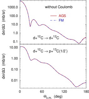
Figure 3: Comparison of momentum- (solid curves) and configuration-space (dashed-dotted curves) results for the deuteron-¹²C scattering at 30 MeV deuteron lab energy. Differential cross sections for elastic scattering and stripping are shown neglecting the Coulomb interaction.

t]

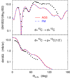
Figure 4: Comparison of momentum- (solid curves) and configuration-space (dashed-dotted curves) results for the deuteron-¹²C scattering at 30 MeV deuteron lab energy. Differential cross sections for elastic scattering and stripping are shown, the former in ratio to the Rutherford cross section $d\sigma_{R}/d\Omega$. The experimental data are from Refs. perrin:77 ; dC30p .

t]

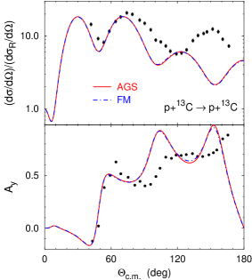
Figure 5: Comparison of momentum- (solid curves) and configuration-space (dashed-dotted curves) results for the proton-¹³C elastic scattering at 30.6 MeV proton lab energy. Differential cross section divided by the Rutherford cross section and proton analyzing power are shown. The experimental data are from Ref. pC30 .

4.2 Comparison with traditional nuclear reaction approaches

The method based on the momentum-space AGS equations has already been used to test the accuracy of the traditional nuclear reaction approaches; limitations of their validity in energy and kinematic range have been estalished. The distorted-wave impulse approximation for breakup of a one-neutron halo nucleus ¹¹Be on a proton target has been tested in Ref. crespo:08a while the adiabatic-wave approximation for the deuteron stripping and pickup reactions ¹¹Be$(p,d){}^{10}$Be, ¹²C$(d,p){}^{13}$C, and ⁴⁸Ca$(d,p){}^{49}$Ca in Ref. nunes:11b . However, one of the most sophisticated traditional approaches is the CDCC method austern:87 . A detailed comparison between CDCC and AGS results is performed in Ref. deltuva:07d . The agreement is good for deuteron-¹²C and deuteron-⁵⁸Ni elastic scattering and breakup. In these cases nucleon-nucleus interactions were given by optical potentials; thus, there was no transfer reaction. A different situation takes place in proton-¹¹Be scattering where ¹¹Be nucleus is assumed to be the bound state of a ¹⁰Be core plus a neutron. In this case, where the transfer channel $d+{}^{10}$Be is open, the CDCC approach lacks accuracy as shown in Ref. deltuva:07d . The semi-inclusive differential cross section for the breakup reaction $p+{}^{11}$Be $\to p+n+{}^{10}$Be was calculated also using two CDCC versions where the full scattering wave function was expanded into the eigenstates of either the $n+{}^{10}$Be (CDCC-BU) or the $p+n$ (CDCC-TR) pair. Neither of them agrees well with AGS over the whole angular regime as shown in Fig. 6. It turns out that, depending on the ¹⁰Be scattering angle, the semi-inclusive breakup cross section is dominated by different mechanisms: at small angles it is the proton-neutron quasifree scattering whereas at intermediate and large angles it is the neutron-¹⁰Be $D$-wave resonance. However, a proper treatment of proton-neutron interaction in CDCC-BU and of neutron-¹⁰Be interaction in CDCC-TR is very hard to achieve since the wave function expansion uses eigenstates of a different pair. No such problem exists in the AGS method that uses simultaneously three sets of basis states and each pair is treated in its proper basis.

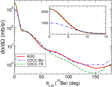
Figure 6: Semi-inclusive differential cross section for the breakup reaction $p+{}^{11}$Be $\to p+n+{}^{10}$Be at lab energy of 38.4 MeV/nucleon. Results obtained with AGS and CDCC methods are compared.

4.3 Beyond standard dynamic models

The standard nucleon-nucleus optical potentials employed in three-body calculations have central and, eventually, spin-orbit parts that are local. This local approximation yields a tremendous simplification in the practical realization of DWBA, CDCC and other traditional approaches that are based on configuration-space representations where the use of nonlocal optical potentials was never attempted. However, nonlocal optical potentials do not yield any serious technical difficulties in the momentum-space representation. Thus, they can be included quite easily in the AGS framework employed by us.

There are very few nonlocal parametrizations of the optical potentials available. We take the one from Refs. giannini ; giannini2 defined in the configuration space as

$$v_{\gamma}(\vec{r}^{\prime},\vec{r})=H_{c}(x)[V_{c}(y)+iW_{c}(y)]+2\vec{S_{\gamma}}\cdot\vec{L_{\gamma}}H_{s}(x)V_{s}(y),$$ (50)

with $x=|\vec{r}^{\prime}-\vec{r}|$ and $y=|\vec{r}^{\prime}+\vec{r}|/2$. The central part has real volume and imaginary surface parts, whereas the spin-orbit part is real; all of them are expressed in the standard way by Woods-Saxon functions. Some of their strength parameters were readjusted in Ref. deltuva:09b to improve the description of the experimental nucleon-nucleus scattering data. The range of the nonlocality is determined by the functions $H_{i}(x)=(\pi\beta_{i}^{2})^{-3/2}\exp{(-x^{2}/\beta_{i}^{2})}$ with the parameters $\beta_{i}$ being of the order of 1 fm.

A detailed study of nonlocal optical potentials in three-body reactions involving stable as well as weakly bound nuclei, ranging from ¹⁰Be to ⁴⁰Ca, is carried out in Ref. deltuva:09b . In order to isolate the nonlocality effect we also performed calculations with a local optical potential that provides approximately equivalent description of the nucleon-nucleus scattering at the considered energy. The nonlocality effect turns out to be very small in the elastic proton scattering from the bound neutron-nucleus system and of moderate size in the deuteron-nucleus scattering. However, the effect of nonlocal proton-nucleus optical potential becomes significant in deuteron stripping and pickup reactions $(d,p)$ and $(p,d)$; in most cases it considerably improves agreement with the experimental data. Examples for $(d,p)$ reactions leading to ground and excited states of the stable nucleus ¹⁷O and one-neutron halo nucleus ¹⁵C are presented in Figs. 7 and 8. We note that in these transfer reactions the proton-nucleus potential is taken at proton lab energy in the proton channel while the neutron-nucleus potential has to be real in order to support the respective bound states.

t]

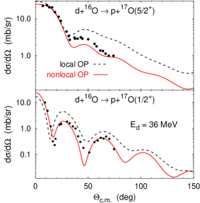
Figure 7: Differential cross section for $(d,p)$ reaction on ¹⁶O at 36 MeV deuteron lab energy leading to ¹⁷O nucleus in the ground state $5/2^{+}$ (top) and first excited state $1/2^{+}$ (bottom). Predictions of nonlocal (solid curve) and local (dashed curve) optical potentials (OP) are compared with the experimental data from Ref. dO25-63 .

t]

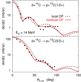
Figure 8: Differential cross section for $(d,p)$ reaction on ¹⁴C at 14 MeV deuteron lab energy leading to one-neutron halo nucleus ¹⁵C in the ground state $1/2^{+}$ (top) and first excited state $5/2^{+}$ (bottom). Curves as in Fig. 7 and the experimental data are from Ref. d14C14p .

Another extension beyond the standard dynamic models includes the AGS method using energy-dependent optical potentials Although such calculations don’t correspond to a rigorous Hamiltonian theory, they may shed some light on the shortcomings of the traditional nuclear interaction models. A detailed discussion of the calculations with energy-dependent optical potentials is given in Ref. deltuva:09a .

5 Summary

We have presented the results of three-body Faddeev-type calculations for systems of three particles, two of which are charged, interacting through short-range nuclear plus the long-range Coulomb potentials. Realistic applications of three-body theory to three-cluster nuclear reactions — such as scattering of deuterons on a nuclear target or one-neutron halo nucleus impinging on a proton target — only became possible to address in recent years when a reliable and practical momentum-space treatment of the Coulomb interaction has been developed. After the extensive and very complete study of $p$-$d$ elastic scattering and breakup, the natural extension of these calculations was the application to complex reactions such as $d$-⁴He, $p$-¹⁷O, ¹¹Be-$p$, $d$-⁵⁸Ni and many others using a realistic interaction such as AV18 between nucleons, and optical potentials chosen at the appropriate energy for the nucleon-nucleus interactions. The advantage of three-body calculations vis-à-vis traditional approximate reaction methods is that elastic, transfer, and breakup channels are treated on the same footing once the interaction Hamiltonian has been chosen. Another advantage of the three-body Faddeev-AGS approach is the possibility to include nonlocal optical potentials instead of local ones as commonly used in the standard nuclear reaction methods; as demonstrated, this leads to an improvement in the description of transfer reactions in a very consistent way across different energies and mass numbers for the core nucleus.

Although most three-body calculations have been performed in momentum space over a broad range of nuclei from ⁴He to ⁵⁸Ni and have encompassed studies of cross sections and polarizations for elastic, transfer, charge exchange, and breakup reactions, coordinate space calculations above breakup threshold are coming to age using the complex scaling method. We have demonstrated here that both calculations agree to within a few percent for all the reactions we have calculated. This is a very promising development that may bring new light to the study of nuclear reactions given that the reduction of the many-body problem to an effective three-body one may be better implemented and understood by the community in coordinate space rather than in momentum space. On the other hand, compared to DWBA, adiabatic approaches, or CDCC, the Faddeev-type three-body methods are computationally more demanding and require greater technical expertise rendering them less attractive to analyze the data. Nevertheless, when benchmark calculations have been performed comparing the Faddeev-AGS results with those obtained using CDCC or adiabatic approaches, some discrepancies were found in transfer and breakup cross sections depending on the specific kinematic conditions. Therefore the Faddeev-AGS approach is imminent in order to calibrate and validate approximate nuclear reaction methods wherever a comparison is possible.

- (1) Alt, E.O., Grassberger, P., Sandhas, W.: Nucl. Phys. B2, 167 (1967)
- (2) Alt, E.O., Mukhamedzhanov, A.M., Nishonov, M.M., Sattarov, A.I.: Phys. Rev. C 65, 064613 (2002)
- (3) Austern, N., Iseri, Y., Kamimura, M., Kawai, M., Rawitscher, G., Yahiro, M.: Phys. Rep. 154, 125 (1987)
- (4) Bruno, M., Cannata, F., D’Agostino, M., Maroni, C., Lombardi, M.: Lett. Nuovo Cimento 27, 265 (1980)
- (5) Chmielewski, K., Deltuva, A., Fonseca, A.C., Nemoto, S., Sauer, P.U.: Phys. Rev. C 67, 014002 (2003)
- (6) Balslev, E., Combes, J. M.: Commun. Math. Phys. 22, 280 (1971)
- (7) C. W. McCurdy, M. Baertschy and T. N. Rescigno: J. Phys. B 373, R137 (2004)
- (8) Cooper, M.D., Hornyak, W.F., Roos, P.G.: Nucl. Phys. A218, 249 (1974)
- (9) Crespo, R., Deltuva, A., Cravo, E., Rodriguez-Gallardo, M., Fonseca, A.C.: Phys. Rev. C 77, 024601 (2008)
- (10) Deltuva, A.: Ph.D. thesis, University of Hannover (2003). URL http://edok01.tib.uni-hannover.de/edoks/e01dh03/374454701.pdf
- (11) Deltuva, A.: Phys. Rev. C 74, 064001 (2006)
- (12) Deltuva, A.: Phys. Rev. C 80, 064002 (2009)
- (13) Deltuva, A.: Phys. Rev. C 79, 021602(R) (2009)
- (14) Deltuva, A., Fonseca, A.C.: Phys. Rev. C 79, 014606 (2009)
- (15) Deltuva, A., Fonseca, A.C., Kievsky, A., Rosati, S., Sauer, P.U., Viviani, M.: Phys. Rev. C 71, 064003 (2005)
- (16) Deltuva, A., Fonseca, A.C., Sauer, P.U.: Phys. Rev. C 71, 054005 (2005)
- (17) Deltuva, A., Fonseca, A.C., Sauer, P.U.: Phys. Rev. C 72, 054004 (2005)
- (18) Deltuva, A., Moro, A.M., Cravo, E., Nunes, F.M., Fonseca, A.C.: Phys. Rev. C 76, 064602 (2007)
- (19) L.D. Faddeev: Zh. Eksp. Teor. Fiz. 39, 1459 (1960), [Sov. Phys. JETP 12, 1014 (1961)]
- (20) Giannini, M.M., Ricco, G.: Ann. Phys. (NY) 102, 458 (1976)
- (21) Giannini, M.M., Ricco, G., Zucchiatti, A.: Ann. Phys. (NY) 124, 208 (1980)
- (22) Glöckle, W.: The Quantum Mechanical Few-Body Problem. Springer-Verlag, Berlin (1983)
- (23) Gorshkov, V.G.: Sov. Phys.-JETP 13, 1037 (1961)
- (24) Goss, J.D., Jolivette, P.L., Browne, C.P., Darden, S.E., Weller, H.R., Blue, R.A.: Phys. Rev. C 12, 1730 (1975)
- (25) Greaves, P.D., Hnizdo, V., Lowe, J., Karban, O.: Nucl. Phys. A179, 1 (1972)
- (26) Johnson, R.C., Soper, P.J.R.: Phys. Rev. C 1, 976 (1970)
- (27) Kievsky, A., Viviani, M., Rosati, S.: Phys. Rev. C 56, 2987 (1997)
- (28) Kievsky, A., Viviani, M., Rosati, S.: Phys. Rev. C 64, 024002 (2001)
- (29) Koersner, I., Glantz, L., Johansson, A., Sundqvist, B., Nakamura, H., Noya, H.: Nucl. Phys. A286, 431 (1977)
- (30) König, V., Grüebler, W., Schmelzbach, P.A., Marmier, P.: Nucl. Phys. A148, 380 (1970)
- (31) Lazauskas, R., Carbonell, J.: Phys. Rev. C 84, 034002 (2011)
- (32) S. P. Merkuriev: Theoretical and Mathematical Physics 8, 798 (1971)
- (33) S. P. Merkuriev: Sov. J. Nucl. Phys. 19, 22 (1974)
- (34) S. P. Merkuriev: Ann. Phys. (N.Y.) 130, 395 (1980)
- (35) S. P. Merkuriev: Acta Physica Austriaca, Supplementum XXIII, 65 (1981)
- (36) S. P. Merkuriev, C. Gignoux, A. Laverne: Ann. Phys 99, 30 (1976)
- (37) N. Moiseyev: Physics Reports 302, 212 (1998)
- (38) Nunes, F.M., Deltuva, A.: Phys. Rev. C 84, 034607 (2011)
- (39) Nuttal, J., Cohen, H. L.: Phys. Rev. 188, 1542 (1969)
- (40) Ohnuma, H., et al.: Nucl. Phys. A448, 205 (1986)
- (41) Perrin, G., Sen, N.V., Arvieux, J., Darves-Blanc, R., Durand, J., Fiore, A., Gondrand, J., Merchez, F., Perrin, C.: Nucl. Phys. A282, 221 (1977)
- (42) Schmid, E.W., Ziegelmann, H.: The Quantum Mechanical Three-Body Problem. Vieweg, Braunschweig (1974)
- (43) Semon, M.D., Taylor, J.R.: Nuovo Cimento A 26, 48 (1975)
- (44) Taylor, J.R.: Nuovo Cimento B 23, 313 (1974)
- (45) Varner, R.L., Thompson, W.J., McAbee, T.L., Ludwig, E.J., Clegg, T.B.: Phys. Rep. 201, 57 (1991)
- (46) M. V. Volkov, N. Elander, E. Yarevsky, S. L. Yakovlev: Europhys. Lett. 85, 30001 (2009)
- (47) Wiringa, R.B., Stoks, V.G.J., Schiavilla, R.: Phys. Rev. C 51, 38 (1995)