The Unimodal Distribution Of Blue Straggler Stars in M75 (NGC 6864)

Abstract

We have used a combination of multiband high-resolution and wide-field ground-based observations to image the Galactic globular cluster M75 (NGC 6864). The extensive photometric sample covers the entire cluster extension, from the very central regions out to the tidal radius, allowing us to determine the center of gravity and to construct the most extended star density profile ever published for this cluster. We also present the first detailed star counts in the very inner regions. The star density profile is well re-produced by a standard King model with core radius $r_{c}\sim 5.4^{\prime\prime}$ and intermediate-high concentration $c\sim 1.75$. The present paper presents a detailed study of the BSS population and its radial distribution. A total number of 62 bright BSSs (with $m_{\rm F255W}\lesssim 21$, corresponding to $m_{\rm F555W}\lesssim 20$) has been identified, and they have been found to be highly segregated in the cluster core. No significant upturn in the BSS frequency has been observed in the outskirts of M75, in contrast to several other clusters studied with the same technique. This observational fact is quite similar to what has been found in M79 (NGC 1904) by Lanzoni et al. (2007a). Indeed the BSS radial distributions in the two clusters is qualitatively very similar, even if in M75 the relative BSS frequency seems to decrease significantly faster than in M79: indeed it decreases by a factor of 5 (from 3.4 to 0.7) within 1 $r_{c}$. Such evidence indicate that the vast majority of the cluster heavy stars (binaries) have already sunk to the core.

1. Introduction

Sandage (1953) first identified a bizarre group of apparently massive young stars immersed in the $\sim 13$ Gyr old population of the globular cluster (GC) M3. They appeared as an extension of the classical hydrogen-burning main sequence (MS), both hotter and more luminous than the stars that define the MS turnoff (TO) point. This was the reason why they were properly named blue straggler stars (BSSs). Being devoid of gas after the burst that formed the bulk of stars, GCs would be unable to form such “young” objects, and their existence in GCs contradicts the current picture of stellar evolution, since massive stars should have evolved into white dwarfs long ago. Their nature has been puzzling for many years, and even today their formation mechanism is not completely understood. Nowadays, BSSs are considered objects more massive than the normal MS stars ($M\sim 1.2M_{\odot}$, see Shara et al., 1997; Ferraro et al., 2006a) that somehow have increased their initial mass. Two explanations for the generation of BSSs are currently leading: mass exchange in primordial binary systems (McCrea, 1964; Zinn & Searle, 1976; Knigge et al., 2009), and stellar mergers induced by collisions in dense environments (Hills & Day, 1976; Leonard, 1989). The two scenarios do not necessarily exclude each other (Bailyn, 1992) and might co-exist in the same GC (see the case of M30, Ferraro et al., 2009).

Gravitational interactions between stars leads to the dynamical evolution of GCs on timescales generally smaller than their ages (Meylan & Heggie, 1997). One signature of such evolution is mass segregation: over time, most massive stars slow down and sink to the cluster core, while lighter stars acquire speed and move to its periphery. Thus, BSSs are expected to preferentially populate the innermost region of star clusters. Because of the stellar crowding, the acquisition of complete samples of BSSs in the core of GCs is a quite difficult task in the optical bands. Conversely, it is easy in the UV bands (Paresce et al., 1991). In fact, due to their high temperatures they are especially bright in the UV, while cool populations such as red giant branch (RGB) stars appear to be quite faint (Ferraro et al., 1997, and references therein). In addition, thanks to the advent of the Hubble Space Telescope (HST) coupled with wide-field imagers on ground–based telescopes, it has become possible to survey the BSS population over the entire extension of GCs. Taking advantage of these possibilities, the BSS radial distribution in several GCs has been already carefully analyzed (Ferraro et al., 1997, 1999, 2003a). The common feature in most of them is that BSSs show a bimodal radial distribution: they appear to be strongly concentrated in the central regions, at intermediate radii the distribution decreases down to a minimum value and then it increases again at outer radii. This behavior has been interpreted in terms of mass segregation by Mapelli et al. (2004, 2006). Notable exceptions to this rule are $\omega$ Centauri (Ferraro et al., 2006a), NGC 2419 (Dalessandro et al., 2008) and, the recently studied, Pal 14 (Beccari et al., 2011), which show a “dynamically young” state of evolution with the BSS population being homogeneously distributed across the entire cluster extension, showing no evidence of central segregation. A different behavior has been found in the GC M79 (Lanzoni et al., 2007a), which instead shows a large concentration of BSSs within the core but no evidence of an upturn in the outerparts of the cluster. This would suggest that the action of mass segregation on the current BSS population is already effective at any distance from the cluster center.

Here we present a complete investigation of the BSS population M75 (NGC 6864). This is a massive and distant GC ($M_{\rm V}=-8.57$, $d\backsimeq 20.9$ kpc; Harris, 1996, 2010 Edition, hereafter HA96) with a moderately high metallicity [Fe/H] $\sim 1.29$ (Carretta et al., 2009), appearing to have a trimodal HB (Catelan et al., 2002) and with a relatively high central density, log$\rho_{0}/(M_{\odot}$ pc${}^{-3})=4.9$ (Pryor & Meylan, 1993) in which BSSs have not been already properly studied. The only previous work, in which BSSs were briefly analyzed was realized by Catelan et al. (2002) as part of their analysis of the overall properties of the Color Magnitude Diagram (CMD) of M75 using ground-based data. The plan of the paper is as follows. In section 2 the photometric data set is presented and discussed. In section 3 we present the determination of the center of gravity and the star density profile of the cluster. In section 4 we discuss the CMD selection and the properties of the BSS sample. In section 5 we draw our conclusions.

2. Data–sets and Analysis

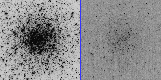
Figure 1.— The cluster center as imaged by the PC ($35^{\prime\prime}\times 35^{\prime\prime}$) of the HST/WFPC2 through the F555W (left panel) and the (UV) F255W (right panel) filter. The optical image is dominated by cool bright red giants which blend together preventing the measure of hot (faint) objects. In the UV image, the brightest objects are HB stars and BSSs and blending effects are not present even in the very central region of the cluster. In this image, hot objects as HB and BSSs are easily identifiable and accurately measurable.

2.1. Observations

The present analysis is based on a combination of two sets of observations:

The High Resolution (HR) data set.— The inner and most crowded region of the cluster has been sampled using the exquisite quality images from the Wide Field Planetary Camera 2 (WFPC2) on board the HST. These data were obtained under program GO 11975 (P.I. F. Ferraro) on March 2009 as part of a major project aimed to census the UV sources in GCs. The cluster was roughly centered on the planetary camera (PC) of the WFPC2 that provides better spatial resolution ($\sim 0^{\prime\prime}$.046 pixel^-1), while the lower resolution ($\sim 0^{\prime\prime}$.1 pixel^-1) wide–field cameras sample the surrounding regions of the cluster. The WFPC2 has a total field of view (FOV) of 150${}^{\prime\prime}\times 150^{\prime\prime}$, which corresponds to a projected area of $15\times 15$ pc² at the distance of M75. The observational material consists of a series of images in 3 carefully selected filters: F255W (4$\times$1200 s), F336W (3$\times$700+1$\times$100 s) and F555W (3$\times$100+1$\times$5 s). Both the high angular resolution and the UV sensitivity of HST are essential to identify the BSSs among the much more luminous (in the classical visible bands) red giants belonging to the cluster. Fig. 1 shows the clear advantage of using UV images to search for hot–objects: it compares two images of the cluster center taken through the F555W filter (left panel) and through the F255W filter (right panel). As can be appreciated, the optical image is dominated by the emission of bright, red (cool) giants, that blend together due to the high crowding conditions, making difficult (if not impossible) the secure identification of BSSs. Conversely, in the UV image (right panel) RGB stars are much dimmer and hot objects like horizontal branch (HB) stars and BSSs, are the brightest sources and therefore easily distinguishable even in the cluster center.

The Wide Field (WF) data set.—The HST/WFPC2 data were complemented with a set of WF images acquired in the $V$ and $I$ bands during an observing run at the 2.2 m ESO-MPI telescope at ESO (La Silla) in 2002 June using the Wide Field Imager (WFI). With a global FOV of $34^{\prime}\times 33^{\prime}$ provided by a mosaic of eight CCD chips (each chip compose of 2050 $\times$ 4100 pixels with a pixel scale of about $\sim 0^{\prime\prime}$.238 pixel^-1) this data covers by far the entire cluster extension (see bottom panel og Fig. 2), allowing exceptional imaging of the outer and less crowded portion of the cluster, which was roughly centered on chip 7.

2.2. Photometry

Each WFPC2 frame was processed through the standard HST-WFPC2 pipeline for bias subtraction, dark correction and flat-fielding. Then, the single–chips were extracted from the 4–chip mosaic, and analyzed separately. Due to vignetting problems affecting the borders of the single–chips, the pixel regions x $\leq 50$; y $\leq 50$ have been excluded from the analysis. Frames obtained with gain = 7e/adu (F225W) and 15 e/adu (F336W, F555W) were available, so care was taken to adjust the various parameters to the applicable gain value for each frame. The brightest, non saturated stars were selected among those having no nearby companions or defects within a few pixels, to construct an analytical Point Spread Function (PSF). In order to fit the star brighteness profile in each frame we adopted a two-component PSF, obtained by combining: (a) an analytical component reproduced by a Moffat (1969) function whose shape has been allowed to vary linearly with the star position in the frame and (a) a numerical component which allows to take into account for the systematic difference between the observed star profile and the analytic approximation. In long exposures, especially in the UV band, a huge amount of cosmic rays were present, making the PSF construction tricky. Accordingly, we combined the UV–images using the IRAF task imcombine (imposing $\it{crreject}$ to eliminate cosmic rays) in order to selected the PSF star candidates in a decontaminated median frame. The stellar photometric reduction was carried out using the DAOPHOTII/ALLFRAME package (Stetson, 1987, 1994). A preliminary photometry was performed in order to construct a list of stars and obtain accurate coordinates for each single frame. We used DAOMATCH/DAOMASTER to determine coordinate transformations for every image to a carefully selected reference one. These transformations were then used by the MONTAGE task routine to create a “master” frame combining the F255W and F336W data in order to eliminate cosmics rays, hot pixels and other spurious sources, and obtain a high signal/noise image for star finding. In our opinion, this filter selection is the best compromise for the detection of both hot and cold sources. We used the DAOPHOT/FIND routine to selected objects in the master image imposing a detection limit $\geq 3\sigma$ and then the entire star list was given as input to ALLFRAME, which performed a simultaneous PSF–photometry of all the individual frames using the coordinate transformation among all the images. Using again DAOMASTER, first, we created a catalog of mean magnitudes of each filter, and then we combined these individual catalogs to obtain a final master one in which the star list includes all the sources detected in at least two filters. As a final step, we transformed the F255W, F336W and F555W instrumental magnitudes into the VEGAMAG photometric system using the procedure described in Holtzman et al. (1995) with the zero points listed in Table 5.1 of the HST Data Handbook.

As far as the reduction of the WFI data is concerned, the images were initially corrected for bias and flat-field with the standard IRAF routines. Then stellar photometry was obtained running DAOPHOTII/ALLFRAME on all the images simultaneously, as describe above. The calibration of the instrumental magnitudes into the VEGAMAG photometric system has been done in 2 successive steps: First, since no photometric standard stars were available, we used the calibrated catalog obtained by Catelan et al. (2002) to link the WFI instrumental magnitudes to the standard Johnson system. With this purpose in mind, we performed a cross correlation between the two catalogs, and selected about 700 stars in common. This sample covers a sufficiently wide range in color to prevent any residual, uncorrected color trend. These selected stars were then used to calibrate the WFI data by means of a least-squares fit. Second, we applied Holtzman et al. (1995) equations 7 and 9 (taking as zero points those presented in their Table 9) to convert the magnitudes from the Johnson to the VEGAMAG system, thus making the WFI dataset photometrically homogeneous with the HST one. In the following, we will therefore adopt the notation $m_{\rm F555W}$ and $m_{\rm F814W}$ to label also the V and I magnitudes of the WFI dataset.

Figure 2.— Upper panel: Map of the HR sample. The positions of all the measured stars are plotted with respect to the center of gravity. The BSSs identified in this sample are marked as large filled circles. The circle at $r=90^{\prime\prime}$ from the cluster center marks the edge of the sample used in the present snalysis. Lower panel: Map of the WF sample. Large filled circles are the identified BSSs. The solid circle at $r=5^{\prime}$ marks the position of the tidal radius. The dashed circle at $900^{\prime\prime}$ from the cluster center delimitate the region adopted to evaluate the background contamination.

2.3. Astrometry

In order to place the HR and WF samples in a common coordinate system we have used astrometric standard stars selected from the new Guide Star Catalog (GSCII). The procedure has been described in previous papers (Ferraro et al., 2003b). We summarize here the main steps: using several hundreds of stars in common between the WFI catalogue and the GSCII, the stars position in each of the eight WFI chips were placed on the absolute astrometric system. For this purpose, we have used CataXcorr, a program developed at the Bologna Observatory (P. Montegriffo, private comunication), to perform roto-translation procedures and allow accurate absolute positioning of the stars. At the end of the procedure, the position residuals were of the order of $\sim 0^{\prime\prime}$.2 in both right ascension ($\alpha$) and declination ($\delta$). Then, the HST catalog was placed on the absolute astrometric system by cross-correlating a few hundred stars in common between the WFI and the WFPC2 FOVs (see Fig. 2). We estimate that the astrometric uncertainty for the WFPC2 stars is less than $\sim 0^{\prime\prime}$.2 in both $\alpha$ and $\delta$.

3. Results

3.1. Center of Gravity

Taking advantage of the knowledge of the exact positions of the stars, even in the innermost central regions, we have estimated the geometrical center ($C_{\rm grav}$) of the star distribution as the barycenter of the within the PC FOV. In doing so, we have performed the iterative procedure described in Montegriffo et al. (1995). In order avoid incompleteness effects and possible statistical fluctuations, we considered stars contained within four circular areas with different radii ($10^{\prime\prime}$, $11^{\prime\prime}$, $12^{\prime\prime}$ and $13^{\prime\prime}$) and three different magnitude cuts ($m_{\rm F555W}=20.5,21$ and $21.5$), adopting as first guess the center reported by HA96. Finally, we simply took the average of the twelve computed values as the best estimate of $C_{\rm grav}$ position, which is located at $\alpha_{\rm j2000}=$20^h 06^m 4^s.85, $\delta_{\rm j2000}=$-21^∘ 55^′ 17^′′.85. This new value for the barycenter of M75 differs slightly ($\Delta\alpha=0.16^{s}$, $\Delta\delta=-1.65^{\prime\prime}$) from the previous one listed in HA96 based on the surface brightness distribution.

Finally, the two catalogs were merged together. Being aware of the superior resolution capabilities of HST and the high effectiveness of the UV observations in detecting BSSs in the crowded central region of the cluster, we have considered only stars measured in the HR sample at $r\leq 90^{\prime\prime}$ from $C_{\rm grav}$, and we have consistently restricted the WF sample to the region $r>90^{\prime\prime}$. Because of the peculiar shape of the WFPC2 FOV, our choice implies that part of the area in the inner $90^{\prime\prime}$ (see top panel of Fig. 2) is covered by neither of the two samples. However, at the same time, this selection minimizes incompleteness effects and stellar blends in the central region of the cluster.

Figure 3.— The optical CMDs for the HR and WF samples. The shaded region ($m_{\rm F555W}>$ 21) delimit the samples excluded for the computation of the star density profile.

At the end of the whole procedure, we ended up with a final catalog fully homogeneous both in magnitudes and coordinates, covering the entire cluster extension. Fig. 3 shows the optical ($m_{\rm F555W}$, $m_{\rm F336W}-m_{\rm F555W}$) and ($m_{\rm F555W}$, $m_{\rm F555W}-m_{\rm F814W}$) CMDs for the HR and WF samples, respectively. A total of 44220 stars are plotted: 30806 in the HR sample and 13414 in the WF sample, respectively. Because of its large extension (reaching $r>25^{\prime}$ from the cluster center) the WF sample is dominated by the Galactic field. These samples have been first used to compute the star density profile.

3.2. Density profile

The dynamical status of a GC can be probed using surface brightness and/or density stellar profiles. However, when evaluating the brightness over small regions, the profiles may be affected by large fluctuations caused by few bright stars. On the other hand, we can take advantage of the fact that we resolve stars even in the innermost region of the cluster and directly build the star density profile, which is likely the most robust tool for determining the cluster structural parameters (Lugger et al., 1995).

Figure 4.— Observed surface density profile (dots) and best–fit King model (solid line). The dotted line indicates the measured level of the background. The parameters of the King model (core radius and concentration) are indicated in the Figure. The location of the cluster core radius (at $r_{\rm t}=5^{\prime\prime}$) is marked by the vertical arrow. The lower panel shows the residuals of the fitting procedure in each radial bin.

Using direct counts, we have therefore determined the projected density profile of M75 for its entire radial extension, from $C_{\rm grav}$ out to $\sim 1000^{\prime\prime}$ $(\sim 100$ pc). To avoid incompleteness effects and keep field contamination as low as possible, we have considered only stars brighter than $m_{\rm F555W}=21$ and located within a $3\sigma$–width selection boxes running along the main evolutionary sequences defined in the CMD by the cluster stars. Following the procedure described by Ferraro et al. (2003b), we have divided our catalog into 22 concentric annuli centered on $C_{\rm grav}$ and each annulus, in turn, has been split in a number of equivalent subsectors. The number of stars lying within each subsector has been counted, averaged and finally divided by the area of the subsector to eventually obtain the mean star density of each annulus. The standard deviation between the subsectors in each annulus has been used as the uncertainty of the star density. The radial density profile thus derived is plotted in Fig. 4 (solid dots), with the abscissas corresponding to the mid-point of each radial bin. The plot clearly shows that the star counts flatten beyond $r\gtrsim 400^{\prime\prime}$. This feature has been used to directly estimate the contribution of the background level, which is shown by the dashed line in Fig. 4. The adopted lower magnitude limit for the density profile counts ($\sim$ MS TO level) imply that all the stars considered in the analysis have approximately the same mass. Accordingly, a mono-mass, isotropic King model has been computed in order to reproduce the observed profile (solid line in Fig. 4). The best fit to our data provides a core radius $r_{c}=5.4^{\prime\prime}$ (which corresponds to $\sim 0.5$ pc) and a concentration parameter $c=1.75$, which would suggest that M75 has not already experienced the core collapse ($c\gtrsim 2$, Meylan & Heggie, 1997). Our results are in perfect agreement with those quoted by McLaughlin & van der Marel (2005), $r_{\rm c}=5.4^{\prime\prime}$ and $c=1.8$, both derived from the surface brightness profile.

Table 1The BSS Population of M75

$Name$	$R.A.$	$Dec.$	$Dist.$	$F255W$	$F336W$	$F555W$	$F814W$
	(degree)	(degree)	(arcsec)
BSS1	301.5202501	-21.9217358	0.401	21.150	20.279	20.002	…..
BSS2	301.5201192	-21.9215229	0.520	20.418	19.653	19.198	…..
BSS3	301.5200227	-21.9216803	0.712	20.343	19.627	19.276	…..
BSS4	301.5200460	-21.9217440	0.740	21.259	20.092	19.601	…..
BSS5	301.5202849	-21.9213937	0.859	21.304	20.198	19.573	…..
BSS6	301.5198820	-21.9213940	1.426	20.827	20.046	19.730	…..
….

3.3. Cluster population selection

The first step to study the projected BSS radial distribution is the appropriate selection of the BSS and the reference populations. In defining the population samples, here we followed the approach already adopted in previous papers of this series (e.g. Ferraro et al., 2003a; Lanzoni et al., 2007a; Dalessandro et al., 2009). We underline that the exact shape of the population selection boxes could slightly vary from cluster to cluster, depending on many factors such as (a) the cluster properties (for instance, the HB morphology and presence of RR Lyrae, which, when observed at random phases, could be locate above or below the HB level an possibly contaminate the brightest portion of the BSS population), (b) the quality of the photometry (which can significantly spread the sequences at the faint end), (c) the necessity to exclude field stars. These differences, however, do not affect the comparison of the population radial distribution.

3.3.1 BSS population

Previous works aimed at studying the BSS population in GCs (see Ferraro et al., 2003a; Lanzoni et al., 2007a; Dalessandro et al., 2009, and references therein) have shown that BSSs are easily distinguished from the cooler stars of the turnoff, SGB and RGB when using UV CMDs. The main reason is that at these wavelengths the cluster light is dominated by hot stars, especially the blue HB and the BSSs. As shown in Fig. 1, HB stars and BSSs are the brightest objects appearing in the UV image, while the contribution from cooler MS, RGB and SGB stars is almost negligible. This is even more clear in the UV CMD shown in Fig. 5. Indeed, the location and morphology of the main evolutionary branches in the UV bands are very different from the classical optical CMD (see Fig. 6). The RGB is very faint and the HB appears as a narrow branch crossing diagonally the CMD.

Figure 5.— Ultraviolet ($m_{\rm F255W}$, $m_{\rm F255W}-m_{\rm F336W}$) CMD for the HR sample. The solid line delimitate the detection limit at $m_{\rm F336W}\sim 22.8$. The selection box used for the definition of the BSSs (plotted as large filled circles) is shown. All the RR Lyrae stars identified in the HR field are marked with large triangles.

In turn, the BSS population defines a nearly vertical sequence spanning $\sim 3$ mag in $m_{\rm F255W}$. They are clearly separable from the fainter TO and SBG stars. For these reasons our primary criterion for the BSS selection is based on the position of stars in the ($m_{\rm F255W},m_{\rm F255W}-m_{\rm F336W}$) plane. However, an unequivocal definition of the faint edge of the BSS population is not simple since the BSS sequence merges smoothly into the MS–TO region without showing any gap or discontinuity. To avoid any possible contamination due to blends, incompleteness and TO and SGB stars in the BSS sample, here we limit our selection criteria to the brightest portion of the BSS sequence. Thus, we have imposed $m_{\rm F225W}\leq 21.3$ as the fainter threshold of the BSS selection box. This limit is nearly one mag brighter than the MS TO in the UV plane.

Figure 6.— Optical ($m_{\rm F555W}$, $m_{\rm F336W}-m_{\rm F555W}$) CMD for the HR sample. The selected populations are plotted with different symbols: RGB (open squares), HB (open circles), known RR Lyrae (open triangles). The BSSs selected from the UV CMD shown in Fig.5 are plotted as filled circles. Note the presence in the BSS region of spurious objects probably due to optical blends of TO stars.

The adopted selection box for the BSSs in the HST sample is shown in Fig. 5. A total of 59 bright-BSSs have been counted in this way. In Fig. 6 the BSSs selected in the UV plane are plotted in the optical CMD (filled circles). This, once again, illustrates the problem of using optical CMDs to identify BSSs in crowded regions. Even with the high resolution achieved with HST, the BSS region can be populated by spurious objects as a result of blending in the dense GC cores. In fact, there are many objects lying in the BSS region that were not classified as genuine BSSs in the UV diagram. We believe that most of them may be considered stellar blends. In the same vein, there are some stars lying very close to the RGB sequence, illustrating that the optical magnitudes may suffer blend/crowding problems.

In order to define a selection box for BSSs in the WF sample, we have adopted the same $m_{\rm F555W}$ magnitude range ($18.5\lesssim m_{\rm F555W}\lesssim 20.2$) as for the HST (Fig. 6), while the red edge has been conservatively chosen in order to limit the effect of the field contamination. Three BSSs have been selected in this way (see Fig. 7). A detailed comparison with the sample of 26 BSS found by Catelan et al. (2002) in M75 was performed. Six of their candidates are outside the region sampled by our observations: they lie in the innermost region ($r<90"$) not covered by the WFPC2 FoV (see top panel of Fig. 2). Of the eight stars found in the area covered by our HST data, only one lies in the BSS selection box. The other seven are SGB, RGB stars well below the BSS sequence in the ($m_{F255W},m_{F255W}-m_{F336W}$) plane. Because of the higher HST spatial resolution and the BSS selection performed in the UV plane, we suggest that these stars are indeed blends in the optical bands. The remaining 12 candidates are located in the external region (with $r>90^{\prime\prime}$): nine of them appears to be SGB or TO stars, well below the selection threshold. One candidate has a magnitude consistent with our magnitude range but it has a color too red to be considered a genuine BSS. Three candidates may be faint-BSS, since they lie along the BSS sequence but they are fainter than our threshold magnitude. In summary, a total of 62 BSSs has been selected in our field of M75, and all of them have been confirmed by visual inspection. The identification, coordinates, distance from the derived $C_{\rm grav}$ and magnitudes of all the selected BSSs are listed in Table 1, which is available in full size in the electronic version of the journal. The spatial distribution of the selected BSSs is shown in Fig. 2. The BSS distribution appears to be highly concentrated within the innermost region of the cluster. In particular, most of the BSS candidates lie within the inner $\sim 15^{\prime\prime}$ (PC FOV).

3.3.2 Reference Populations

[!b]

Figure 7.— Left panel: CMD of the inner $300^{\prime\prime}$ of the WF sample. The selection boxes used to define the BSS and RGB samples are plotted. Right panel: CMD of the field region, corresponding to the most external region ($r>900^{\prime\prime}$) of the WF sample (see Fig. 2 lower panel), with the population selection boxes superimposed.

In order to quantify this visual impression we need to compare the BSS distribution to that of a reference population, which is expected to display a non–peculiar radial trend within the cluster. As in previous papers (see Ferraro et al., 2003a; Dalessandro et al., 2008), we have adopted the RGB and HB stars as reference populations. The selection of the RGB stars has been performed in the optical ($m_{\rm F555W},m_{\rm F336W}-m_{\rm F555W}$) and ($m_{\rm F555W},m_{\rm F555W}-m_{\rm F814W}$) planes, for the HR and WF samples, respectively. For both samples a magnitude threshold at $m_{\rm F555W}\lesssim 20$ has been adopted. The selected RGB stars are shown as open squares in Fig. 6 and 7. The color limits of the boxes have been chosen in order to follow the morphology of the RGB in each plane and in order to minimize the contamination from AGB stars and field outliers. Slightly different assumptions on the selection boxes would have included or excluded a few objects without affecting the results of this analysis. Following this approach, we selected 1434 RGB in the HR sample and 241 RGB in the WF sample within $r<300^{\prime\prime}$, this radial limit corresponding to the estimated tidal radius of M75 (see Sect. 3.2). The HB stars have been selected essentially in the UV plane for the HR sample, and a careful analysis has been performed in order to check that all these objects lay also on the HB in the optical plane. The final selection is shown in Fig. 6 where HB stars are plotted as large open circles. The same symbols are used to mark the HB population in the WF sample (left panel of Fig. 7), which has been selected using the optical ($m_{\rm F555W},m_{\rm F555W}-m_{\rm F814W}$) plane. We carefully identified all the known RR Lyrae stars (Corwin et al., 2003) lying in our FOV. 32 RR Lyrae stars have been found and they are marked as open triangles in Fig. 5, 6, and 7. The total number of HB stars is 425 (29 of them are RR Lyrae) for the HR sample and 95 (3 RR Lyrae) for the WF sample ($r<300^{\prime\prime}$).

Figure 8.— Cumulative radial distribution of BSSs (solid line) and RGB stars (dashed line) as a function of the projected distance from the cluster $C_{\rm grav}$ for the combined HR+WF sample. The location of the cluster tidal radius is marked by the vertical arrow.

3.3.3 Field Decontamination

The close inspection of the CMDs (in particular the diagram shown in the right–hand panel of Fig. 7) suggests that the selected populations can be affected by contamination from field stars. As expected, the relative contribution of background star increases progressively at large distance from the center, where the cluster population significantly decreases and the Galaxy field population is dominant. In order to quantitatively evaluate this effect we took advantage of the large FOV of the WF sample. Hence, we have used the outermost portion ($r\geq 900^{\prime\prime}$) of the WFI data set, well beyond the tidal radius (see Fig. 2), to statistically subtract the background contribution. Accordingly, we have estimated the area of this region ($\sim 500$ arcmin²) and counted the number of stars lying within the corresponding BSS, HB and RGB selection boxes shown in Fig. 7. The estimated contamination is roughly 0.008, 0.3 and 0.53 stars/arcmin² for BSSs, HB and RGB stars, respectively.

3.4. The BSS Radial Distribution

The cumulative radial distribution for the 62 bright-BSSs and the 1675 RGB stars are plotted in Fig. 8 as a function of their projected distance from the cluster center. It is evident from the plot that the BSSs (solid line) are more centrally concentrated than RGB stars (dashed line). In fact, approximately $50\%$ of the BSSs are located in the first $\sim 4^{\prime\prime}$ ($0.75r_{\rm c}$), while only $\sim 10\%$ RGB stars are enclosed within the same distance. Hence, there is a preliminary evidence that the radial distribution of the BSS is quite different from that of the normal cluster populations. We used a Kolmogorov-Smirnov (KS) test in order to check the null hypothesis that the radial distributions of the BSS and RGB populations are identical, finding a probability of $\sim 10^{-6}\%$. Thus, the BSS population in M75 has a different radial distribution than the RGB stars with more than $99\%$ probability.

Table 2Number Counts of BSSs, RGB, and HB stars, and Fraction of Sampled Luminosity in each annulus defined in section 3.4.

$r_{\rm i}^{\prime\prime}$	$r_{\rm e}^{\prime\prime}$	$N_{\rm BSS}$	$N_{\rm RGB}$	$N_{\rm HB}$	$L_{\rm samp}/L_{\rm samp}^{\rm tot}$
0	5	33	266	77	0.16
5	10	9	311	82	0.20
10	15	5	248	65	0.15
15	40	7	400	132	0.22
40	60	3	123(1)	44	0.08
60	90	2	86(1)	25(1)	0.06
90	150	3	137(7)	50(4)	0.09
150	300	0	104(31)	45(18)	0.04

For a more quantitative analysis of the BSS distribution, we have followed the procedure described in previous papers (see e.g., Ferraro et al., 2004; Sabbi et al., 2004) and computed the specific frequencies $F^{\rm BSS}_{\rm RGB}=N_{\rm BSS}/N_{\rm RGB}$ and $F^{\rm BSS}_{\rm HB}=N_{\rm BSS}/N_{\rm HB}$, where $N_{\rm BSS}$, $N_{\rm RGB}$ and$N_{\rm HB}$ represent the number of BSSs, RGB and HB stars, respectively. In doing this, the surveyed area has been divided into a set of concentric annuli and the number of BSSs, RGB and HB stars contained in each annulus were counted. Star counts and the corresponding number of field stars (in parenthesis) for each population in each annulus are listed in Table 2. The specific frequencies as a function of the projected distance from $C_{\rm grav}$ are shown in Fig. 9. For sake of completeness, the bottom panel plots the behavior of the ratio $N_{\rm HB}/N_{\rm RGB}$, showing that the selected reference populations share the same radial distribution. This farther demonstrates that the BSS radial distribution is peculiar independently of the adopted reference population. Indeed, both $N_{\rm BSS}/N_{\rm HB}$ and $N_{\rm BSS}/N_{\rm RGB}$ show clearly a unimodal trend: the highest value is reached in the innermost annulus ($F^{\rm BSS}_{\rm RGB}\sim 0.13$ and $F^{\rm BSS}_{\rm HB}\sim 0.42$), and then the distribution decreases steeply, remaining flat as $r$ increases.

Figure 9.— Radial distribution of the population ratios $N_{\rm BSS}/N_{\rm HB}$, $N_{\rm BSS}/N_{\rm RGB}$ and $N_{\rm HB}/N_{\rm RGB}$ (top, middle and bottom, respectively) as a function of the radial distance from the cluster center in core radius units.

As a final check, we have computed the double normalized ratios (or relative frequency) for BSSs and RGB stars, i.e, the ratio of the fractional number of stars in a given evolutionary phase (BSS, RGB) to the fractional sampled luminosity in each annulus, as defined by Ferraro et al. (1993):

$$R_{\rm BSS}=(N_{\rm BSS}/N^{\rm tot}_{\rm BSS})/(L_{\rm samp}/(L_{\rm samp}^{\rm tot}),$$ (1)

$$R_{\rm RGB}=(N_{\rm RGB}/N^{\rm tot}_{\rm RGB})/(L_{\rm samp}/(L_{\rm samp}^{\rm tot}).$$ (2)

The sampled luminosity in each annulus has been obtained by integrating the best–fitting King profile (Fig. 4), and appropriately scaling to the effective area covered by the observations in each annulus. The fraction of sampled to total luminosity is reported in the last column of Table 2. The relative frequency of the BSSs is plotted against radius in Fig. 10, together with that of RGB stars for comparison. As the figure shows, $R_{\rm RGB}$ is essentially uniform over the surveyed area, with a value close to unity. This behavior is exactly what is expected on the basis of the stellar evolution theory, since the number of stars in any post-MS phase scales linearly with the total luminosity of the parent population (Renzini & Buzzoni, 1986). This implies that a “normal” (i.e, non segregated) post-MS population scales as the cluster luminosity at any distance from the center, exactly as found for RGB stars. In contrast, BSSs follow a different radial distribution. Their relative frequency reaches a maximum value at the center of the cluster and decreases to a minimum value at a distances $\sim 5r_{\rm c}$ ($\sim 25^{\prime\prime}$ from $C_{\rm grav}$), and remains approximately constant outwards. This behavior fully confirms that the BSS radial distribution in M75 is not bimodal.

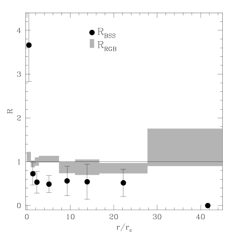
Figure 10.— Radial distribution of the BSS (large filled circles) and RGB (gray regions) relative frequencies as defined in eq. (1) and (2) as a function of the radial distance in units of core radius ($r_{\rm c}=5^{\prime\prime}$). The vertical width of the gray regions correspond to the error bars.

4. Discussion and Conclusions

We have studied the brightest portion ($m_{\rm F225W}\leq 21.3$, roughly corresponding to $m_{\rm F555W}\leq 20.2$) of the BSS population in M75. We have identified a total of 62 objects over a region that covers the entire cluster extension. The BSS population has been found to be highly segregated toward the cluster center: indeed, approximately 60% of the entire BSS population is found within the cluster core, while only $\sim 10-15\%$ of RGB and HB stars are counted in the same region. This suggests a significant overabundance of BSSs in the center, as also confirmed by the fact that the BSS relative frequency ($R_{\rm BSS}$) within $r_{\rm c}$ is roughly 3.5 times larger than expected for a normal (non-segregated) population on the basis of the sampled light (see Fig. 10). This value is one of the largest ever measured in the GCs studied so far with a similar approach. For example it is larger than that measured in M79 ($\sim 2.9$; Lanzoni et al., 2007a), M3 ($\sim 1.5$; Ferraro et al., 1997), 47 Tuc ($\sim 2.6$; Ferraro et al., 2004), and M5 ($\sim 2.7$; Lanzoni et al., 2007b).

Notably, at odds with most of those clusters, no significant upturn of the distribution at large radii has been detected in M75. Indeed the distribution found here is similar to that discovered by Lanzoni et al. (2007a) in M79: both these clusters show a central peak and a rapidly decreasing BSS specific frequency (within a few $r_{c}$), without any evidence of a rising branch in the outskirts. As discussed in Lanzoni et al. (2007a) for the case of M79, the absence of an external upturn in the BSS radial distribution is not an effect of low statistics, since other clusters show the external upturn in spite of a BSS population smaller or similar to that measured in M75 (see the case of NGC 6752 by Sabbi et al., 2004).

In order to further explore the similarity between the BSS distribution in M75 and M79, we directly compare them in Fig. 11. As can be seen, although the behavior of the two distributions is qualitatively similar, the decreasing trend of $R_{\rm BSS}$ in M75 appears to be 1) significantly sharper in the central region, where it decreases by a factor of 5 (from 3.4 to 0.7) within just 1 $r_{\rm c}$ from the cluster center, and 2) somehow less steeper in the external regions, where it possibly define a sort of plateau.

Dynamical simulations (see Mapelli et al., 2004, 2006; Lanzoni et al., 2007a) have been used to derive some hints about the origin of the BSS radial distribution. For example they demonstrated that the external rising branch of the BSS radial distribution observed in many GCs (M3, 47 Tuc, NGC 6752 and M5) cannot be due to BSSs which originate in the core and then kicked out in the outer regions. Instead it may be the consequence of binary systems evolving in isolation in the cluster outskirts. In particular the measure of the so-called radius of avoidance ($r_{\rm avoid}$, which indicates the distance at which the heavy stars like binaries have sunk to the cluster core) has been used to measure the efficiency of the dynamical friction in the cluster. Following the procedure describe by Beccari et al. (2006), we have derived $log\rho_{0}=5.0\,M_{\odot}\,{\rm pc}^{-3})$ for the central density of M75. Moreover, adopting the best–fit King model and assuming a velocity dispersion $\sigma_{0}=10.3$ km s^-1 (McLaughlin & van der Marel, 2005), 12 Gyr as the cluster age and the aforementioned computed value for the the central density, we have used the dynamical friction formula (see e.g., eq. 1 in Mapelli et al., 2006) to estimate $r_{\rm avoid}$ for M75, which is $\sim 17r_{\rm c}$. Hence, on the basis of this theoretical estimate, we would expect a rising branch of the BSS population in the bins with $r>r_{\rm avoid}$ $\sim 17r_{\rm c}$, which is instead not observed. We note that only 3 BSS have been observed in the annulus between $90^{\prime\prime}<r<150^{\prime\prime}$, and that 6 are needed to increase the $R$ value to 1 in Fig. 10. The situation is similar in the most external bin $150^{\prime\prime}<r<300^{\prime\prime}$, where 2 BSS are expected and 0 are observed. Admittedly these are very small numbers largely dominated by statistical fluctuations. However, from a purely observational point of view, it is quite unlikely that we have lost a total of 5 BSS in such uncrowded region. On the other hand, we the estimate of $r_{\rm avoid}$ is very sensitive to velocity dispersion ($\varpropto\sigma^{3}$), which in the case of M75 has an uncertainty $\sim 20\%$, meaning that $r_{\rm avoid}\sim 24r_{\rm c}$ may be achieved within the errors. It becomes clear that more accurate estimates of dynamical parameters are needed to better clarify this point.

Figure 11.— Radial distribution of the double normalized ratio $R_{\rm BSS}$ for M75 (filled circles) compared to that measured in M79 (open circles) by Lanzoni et al. (2007a), plotted as a function of the radial distance from the cluster center in core radius units.

The present study further demonstrates that BSS surveys covering the full radial extent of GCs are powerful tools to determine how common bimodality is and its connection to the cluster dynamical history. A survey of physical and chemical properties for a representative number of BSSs in M75 as those performed by Ferraro et al. (2006b) in 47 Tuc and Lovisi et al. (2010) in M4 should clarify the formation processes of these stars.

References

- Bailyn (1992) Bailyn, C. D. 1992, ApJ, 392, 519
- Beccari et al. (2006) Beccari, G., Ferraro, F. R., Possenti, A., et al. 2006, AJ, 131, 2551
- Beccari et al. (2011) Beccari, G., Sollima, A., Ferraro, F. R., et al. 2011, ApJ, 737, L3
- Catelan et al. (2002) Catelan, M., Borissova, J., Ferraro, F. R., et al. 2002, AJ, 124, 364
- Carretta et al. (2009) Carretta, E., Bragaglia, A., Gratton, R., D’Orazi, V., & Lucatello, S. 2009, A&A, 508, 695
- Corwin et al. (2003) Corwin, T. M., Catelan, M., Smith, H. A., et al. 2003, AJ, 125, 2543
- Dalessandro et al. (2008) Dalessandro, E., Lanzoni, B., Ferraro, F. R., et al. 2008, ApJ, 681, 311
- Dalessandro et al. (2009) Dalessandro, E., Beccari, G., Lanzoni, B., et al. 2009, ApJS, 182, 509
- Ferraro et al. (1993) Ferraro, F. R., Pecci, F. F., Cacciari, C., et al. 1993, AJ, 106, 2324
- Ferraro et al. (1997) Ferraro, F. R., Paltrinieri, B., Fusi Pecci, F., et al. 1997, A&A, 324, 915
- Ferraro et al. (1999) Ferraro, F. R., Paltrinieri, B., Rood, R. T., & Dorman, B. 1999, ApJ, 522, 983
- Ferraro et al. (2001) Ferraro, F. R., D’Amico, N., Possenti, A., Mignani, R. P., & Paltrinieri, B. 2001, ApJ, 561, 337
- Ferraro et al. (2003a) Ferraro, F. R., Sills, A., Rood, R. T., Paltrinieri, B., & Buonanno, R. 2003a, ApJ, 588, 464
- Ferraro et al. (2003b) Ferraro, F. R., Possenti, A., Sabbi, E., et al. 2003b, ApJ, 595, 179
- Ferraro et al. (2004) Ferraro, F. R., Sollima, A., Pancino, E., et al. 2004, ApJ, 603, L81
- Ferraro et al. (2006a) Ferraro, F. R., Sollima, A., Rood, R. T., et al. 2006a, ApJ, 638, 433
- Ferraro et al. (2006b) Ferraro, F. R., Sabbi, E., Gratton, R., et al. 2006b, ApJ, 647, L53
- Ferraro et al. (2009) Ferraro, F. R., Beccari, G., Dalessandro, E., et al. 2009, Nature, 462, 1028
- Harris (1996) Harris, W. E. 1996, VizieR Online Data Catalog, 7195, 0
- Hills & Day (1976) Hills, J. G., & Day, C. A. 1976, Astrophys. Lett., 17, 87
- Holtzman et al. (1995) Holtzman, J. A., Burrows, C. J., Casertano, S., et al. 1995, PASP, 107, 1065
- Knigge et al. (2009) Knigge, C., Leigh, N., & Sills, A. 2009, Nature, 457, 288
- Lanzoni et al. (2007a) Lanzoni, B., Sanna, N., Ferraro, F. R., et al. 2007a, ApJ, 663, 1040
- Lanzoni et al. (2007b) Lanzoni, B., Dalessandro, E., Ferraro, F. R., et al. 2007b, ApJ, 663, 267
- Leonard (1989) Leonard, P. J. T. 1989, AJ, 98, 217
- Lovisi et al. (2010) Lovisi, L., Mucciarelli, A., Ferraro, F. R., et al. 2010, ApJ, 719, L121
- Lugger et al. (1995) Lugger, P. M., Cohn, H. N., & Grindlay, J. E. 1995, ApJ, 439, 191
- Meylan & Heggie (1997) Meylan, G., & Heggie, D. C. 1997, A&A Rev., 8, 1
- McCrea (1964) McCrea, W. H. 1964, MNRAS, 128, 147
- McLaughlin & van der Marel (2005) McLaughlin, D. E., & van der Marel, R. P. 2005, ApJS, 161, 304
- Mapelli et al. (2004) Mapelli, M., Sigurdsson, S., Colpi, M., et al. 2004, ApJ, 605, L29
- Mapelli et al. (2006) Mapelli, M., Sigurdsson, S., Ferraro, F. R., et al. 2006, MNRAS, 373, 361
- Moffat (1969) Moffat, A. F. J. 1969, A&A, 3, 455
- Montegriffo et al. (1995) Montegriffo, P., Ferraro, F. R., Fusi Pecci, F., & Origlia, L. 1995, MNRAS, 276, 739
- Paresce et al. (1991) Paresce, F., Meylan, G., Shara, M., Baxter, D., & Greenfield, P. 1991, Nature, 352, 297
- Pryor & Meylan (1993) Pryor, C., & Meylan, G. 1993, Structure and Dynamics of Globular Clusters, 50, 357
- Renzini & Buzzoni (1986) Renzini, A., & Buzzoni, A. 1986, Spectral Evolution of Galaxies, 122, 195
- Sabbi et al. (2004) Sabbi, E., Ferraro, F. R., Sills, A., & Rood, R. T. 2004, ApJ, 617, 1296
- Sandage (1953) Sandage, A. R. 1953, AJ, 58, 61
- Shara et al. (1997) Shara, M. M., Saffer, R. A., & Livio, M. 1997, ApJ, 489, L59
- Stetson (1987) Stetson, P. B. 1987, PASP, 99, 191
- Stetson (1994) Stetson, P. B. 1994, PASP, 106, 250
- Zinn & Searle (1976) Zinn, R., & Searle, L. 1976, ApJ, 209, 734