Nonlinear dynamics of a regenerative cutting process

Abstract

We examine the regenerative cutting process by using a single degree of freedom non-smooth model with a friction component and a time delay term. Instead of the standard Lyapunov exponent calculations, we propose a statistical 0-1 test analysis for chaos detection. This approach reveals the nature of the cutting process signaling regular or chaotic dynamics. For the investigated deterministic model we are able to show a transition from chaotic to regular motion with increasing cutting speed. For two values of time delay showing the different response the results have been confirmed by the means of the spectral density and the multiscaled entropy.

1 Introduction

A cutting process is a basic machining technology to obtain the surface of the assumed parameters. In certain working conditions it can be disturbed by chatter appearing as unexpected waves on the machined surface of a workpiece. The appearance of chatter was noticed and described by Taylor in the beginning of 20th century Taylor1907 . But the first approaches towards explanations of this phenomenon came about 50 years later through the analysis of self-sustained vibrations Arnold1946 , regenerative effects Tobias1958 , structural dynamics Tlusty1963 ; Merit1965 , and, finally, the dry friction phenomenon Wu1985a ; Wu1985b . Consequently, elimination and stabilization of the associated oscillations have become of high interest in science and technology Altintas2000 ; Warminski2003 ; Insperger2006 . The plausible adaptive control concept, based on relatively short time series Ganguli2007 , has been studied to gain deeper understanding.

Recently, apart from the widely developed chatter vibrations chaotic oscillations caused by various system nonlinearities were predicted and detected Grabec1988 ; Tansel1992 ; Gradisek1998a ; Gradisek1998b ; Marghitu2001 ; Litak2002 ; Fofana2003 ; Gradisek2002 ; Litak2004 . The recent technological demand is to improve the final surface properties of the workpiece and to minimize the production time with higher cutting speeds Stepan2003 . Thus a better understanding of the physical phenomena associated with a cutting process becomes necessary Martinez2009 . In this paper we will continue the work on chaotic instabilities in cutting processes proposing the 0-1 test Gottwald2004 ; Gottwald2005 ; Falconer2007 ; Gottwald2009a ; Gottwald2009b as a tool identifying a possible chaotic solution Litak2009 .

This paper is organized as follows. After the present introduction (Sec. 1) we describe the model in Sec. 2. In Sec. 3 we provide the results of the simulations and corresponding power spectral densities (PSD) while in Sec. 4 the 0-1 test is applied and, subsequently, the findings are confirmed by means of the multiscale entropy (Sec. 5). The paper ends with conclusions (Sec. 6).

2 The model

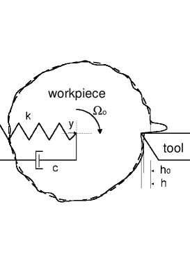
Figure 1: Physical model of a regenerative cutting process Litak2002 .

A regenerative cutting process may exhibit a wide range of complex behavior due to frictional effects Warminski2003 ; Grabec1988 , structural nonlinearities Pratt2001 and delay dynamics Litak2002 ; Fofana2003 ; Stepan2001 ; Wang2006 ; Litak2008 . Moreover it may also involve loss of contact between the tool and the workpiece. The following equations model the regenerative cutting process and the mentioned properties.

After the first pass of the tool, the cutting depth can be expressed as

$$h(t)=h_{0}-y(t)+y(t\!-\!\tau),$$ (1)

where $y(t\!-\!\tau)$ corresponds to the position of the workpiece during the previous pass, and $\tau$ is the time delay scaled by the period of revolution of the workpiece $2\pi/\Omega_{0}$ (Fig. 1). The motion of the workpiece can be determined from the model proposed by Stépán Stepan2001

$$\ddot{y}+2\gamma\dot{y}+\omega_{0}^{2}y=\frac{1}{m}{\rm sgn}(v_{0}\!-\!\dot{y})\big{(}F_{y}(h)-F_{y}(h_{0})\big{)},$$

$$F_{y}(h)=\Theta(h)c_{1}wh^{3/4},$$ (2)

$$\dot{y}(t^{+})=-\beta\dot{y}(t^{-}),$$

where $\omega_{0}=\sqrt{k/m}$ is the frequency of free vibration, $v_{0}$ is the feed velocity, and $2\gamma=c/m$ is the damping coefficient. $F_{y}(h)$ is the thrust force, which is the horizontal component of the cutting force, and $m$ is the effective mass of the workpiece. The thrust force $F_{y}$ is based on dry friction between the tool and the chip. It is assumed to have a power law dependence on the actual cutting depth $h$ and to be proportional to the chip width $w$ and a friction coefficient $c_{1}$. $\Theta(\cdot)$ denotes the Heaviside step function. The restitution parameter $\beta=0.75$ is associated with the impact after contact loss, while $t^{-}$ and $t^{+}$ denotes the time instants before and after the impact. Substituting Eq. (1) into Eqs. (2) we derive a delay differential equation (DDE) for the workpiece motion $y(t)$. Plugging its solution into Eq. (1) results in the history of cutting depth $h(t)$.

3 Simulation results

The non-smooth model equations are solved by a simple Euler integration scheme. The used parameters Litak2002 ; Litak2008 are presented in Table 1.

Table 1: Parameters used in the model

Parameter	Value
initial cutting depth $h_{0}$	$10^{-3}$ m
frequency of free vibration $\omega_{0}$	816 rad/s
damping coefficient $c$	$86$ Ns/m
effective mass of the workpiece $m$	17.2 kg
friction coefficient $c_{1}$	$1.25\times 10^{9}$ N/m2
chip width $w$	$3.0\times 10^{-3}$ m

Furthermore, the feed velocity $v_{0}$ has been assumed to be fairly large so that $v_{0}\!>\!\dot{y}$. Note that, in this case, the system nonlinearities are limited to the exponential dependence of the cutting force on the chip thickness and to the contact loss between the tool and workpiece.

a)

b)

Figure 2: Time series of cutting depth $h(t)$ for (a) time delay $\tau=1.8$ ms and (b) $\tau=2.1$ ms (sampling time $\Delta t=1$ ms with an integration step $\Delta t$/$10^{3}$=1$\mu$s) indicating regular and chaotic motion, respectively. The time series are plotted by sampling points.

The corresponding time series for two choices of the time delay parameter $\tau=1.8$ and 2.1 ms are presented in Fig. 2. These series have been plotted with points. On the first sight one can notice that both solutions are complex but the Fig. 2a shows points grouped in selected lines while the distribution of time history points of Fig. 2b looks more random. In Fig. 2b $h$ reaches negative values that signal that the contact between the tool and the workpiece is lost.

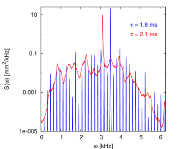
Figure 3: Power spectral density $S(\omega)$ for two chosen delay times. A broad band spectral density indicates chaotic / stochastic dynamics whereas sharp peaks imply regular motion.

The power spectral densities (PSD) of cutting depth $S(\omega)={2\pi}\!/{T}\,|{\cal F}\{h(t)\}|^{2}$ for the two chosen delay times ($\tau=1.8$ ms and $\tau=2.1$ ms) indicate a transition from regular to chaotic motion. The sharp peaks in Fig. 3 belong to a high-periodic orbit (regular motion) whereas the broad spectrum indicates chaotic dynamics.

Both power spectra are dominated by a main peak. In case of regular motion its position belongs to the delay time $\tau=1.8$ ms while in case of chaotic dynamics the time scale belonging to the peak ($t_{p}\approx 2.0$ ms) is smaller than the delay time $\tau=2.1$ ms. This smaller value could be a consequence of a tool-workpiece contact loss. Based on that we take a closer look on other measures to characterize the model’s dynamics and use a 0-1 test for chaos to display a possible transition from regular to chaotic motion with increasing delay time $\tau$.

4 Application of 0-1 test

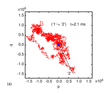
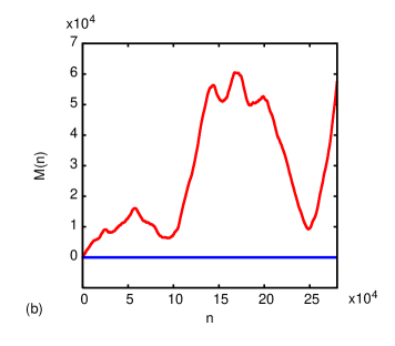
Figure 4: (a) For regular motion ($\tau=$ 1.8 ms) trajectories in $(p,q)$ stay bounded around the initial point ’1’. For chaotic time series ($\tau=2.1$ ms) trajectories in $p$ and $q$ coordinates show Brownian motion-like behavior. (b) Thus the mean square displacement $M(n)$ increases with time. For estimation of $p_{n}$ and $q_{n}$, Eqs. (3), we used $c_{0}=0.7$ and for $M(n)$ and $K$, Eqs. (4) and (5), the upper limits of $N$, $n$ are $N_{max}=40000$, $n_{max}=280000$, respectively.

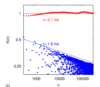
Figure 4: (c) For regular dynamics ($\tau=1.8$ ms) the $K$-value converges towards zero with increasing time. For chaotic dynamics ($\tau=2.1$ ms) $K$ stays close to 1.

Based on the time series $\{\tilde{h}_{j}\}$ which is a discretization of the solution $h(t)$ of the DDE normalized by its standard deviation, we define dimensionless displacements in the $(p,q)$-plane in the following way Gottwald2004 ; Gottwald2005 ; Litak2009

$$p_{n}=\sum_{j=0}^{n}\tilde{h}_{j}\cos(jc_{0}),\hskip 17.07182ptq_{n}=\sum_{j=0}^{n}\tilde{h}_{j}\sin(jc_{0}),$$ (3)

where $c_{0}$ is a constant. In this way regular dynamics is related to a bounded motion while any chaotic dynamics leads to an unbounded motion in the $(p,q)$-plane Gottwald2004 , see Fig. 4a.

To obtain a quantitative description of the examined system we perform calculations of the asymptotic properties defined by the total mean square displacement (MSD) $M(n)$, Fig. 4b, and finally we obtain the growth rate $K$ in the limit of large times

$$M(n)=\lim_{N\rightarrow\infty}\frac{1}{N}\sum_{j=1}^{N}\big{[}\left(p_{j+n}\!-\!p_{j}\right)^{2}+\left(q_{j+n}\!-\!q_{j}\right)^{2}\big{]},$$ (4)

$$K=\lim_{n\rightarrow\infty}\frac{\ln(M(n)+1)}{\ln n}.$$ (5)

For almost all values of the constant $c_{0}$ the parameter $K$ is approaching asymptotically 0 or 1 for regular or chaotic motion, respectively.

Note, practically, one has to truncate the sums in Eq. (4). Thus we derived $K\approx 0.21$ for $\tau=1.8$ ms and $K\approx 1.09$ for $\tau=2.1$ ms, which supports the first impression gained from the time series themselves, Fig. 2a and b. Note further that for delay time $\tau=1.8$ ms, $K$ decays with increasing $n$ on much smaller values, Fig. 4c, which corroborates the result pointing towards regular motion.

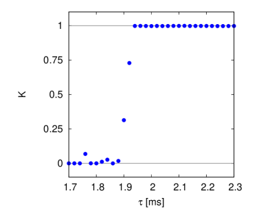
Figure 5: $K$-values for different delay times $\tau$ indicate a transition from regular to chaotic dynamics in the region of 1.9 ms.

Note that, the parameter $c_{0}$ acts like a frequency in a spectral calculation, cp. Eqs. (3). If it is badly chosen, $c_{0}/{\Delta t}$ resonates with one frequency of the process dynamics $\tilde{h}(t)$. Such a frequency belongs to a a peak in the PSD, Fig. 3. In the 0-1 test regular motion would yield a ballistic behavior in the $(p,q)$-plane and the corresponding quadratic growth of MSD results in an asymptotic growth rate. The disadvantage of the test, its strong dependence on the chosen parameter $c_{0}$, could be overcome by a proposed modification. Gottwald and Melbourne Gottwald2005 ; Gottwald2009a suggest to take several randomly chosen values of $c_{0}$ and compute the median of the belonging $K$-values. Particularly, in Ref. Gottwald2009a the problems of averaging over $c_{0}$ as well as sampling the data points are discussed extensively. We followed this approach Gottwald2009a ; Krese2012 , which improves the convergence of the test (Fig. 4c) without the consideration of longer time series, to find the time delay $\tau$ leading to chaos (see Fig. 5). We defined a modified square displacement $D(n)$ which exhibits the same asymptotic growth

$$D(n,c_{0})=M(n,c_{0})-V_{osc}(n,c_{0}),$$ (6)

where the oscillatory term $V_{osc}(n,c_{0})$ can be expressed by

$$V_{osc}(n,c_{0})=E[\tilde{h}]^{2}\frac{1-\cos(nc_{0})}{1-\cos(c_{0})},$$ (7)

and $E[\tilde{h}]$ denotes the average of examined time series $\tilde{h}_{i}$

$$E[\tilde{h}]=\frac{1}{N_{max}}\sum_{i=1}^{N_{max}}\tilde{h}_{i},$$ (8)

where $N_{max}$ is the number of $\tilde{h}_{i}$ elements. Consequently, the oscillatory behavior is subtracted from the MSD $M(n,c_{0})$ and the regression analysis of the linear growth of $D(n,c_{0})$ (Eq. 6) with increasing $n$ is performed using the linear correlation coefficient which determines the value of $K_{c_{0}}$.

$$K_{c_{0}}=\frac{{\rm cov}({\bf X},{\bf D}(c_{0}))}{\sqrt{{\rm var}({\bf X}){\rm var}({\bf D}(c_{0})})},$$ (9)

where vectors ${\bf X}$=[1, 2, …, $n_{max}$], and ${\bf D}(c_{0})$= [$D(1,c_{0})$, $D(2,c_{0})$, …., $D(n_{max},c_{0})$].

The covariance ${\rm cov}({\bf x},{\bf y})$ and variance ${\rm var}({\bf x})$, for arbitrary vectors ${\bf x}$ and ${\bf y}$ of $n_{max}$ elements, and the corresponding averages $E[x]$ and $E[y]$ respectively, are defined

$${\rm cov}({\bf x},{\bf y}) = \frac{1}{n_{max}}\sum_{n=1}^{n_{max}}(x(n)-E[x])(y(n)-E[y]),$$

$${\rm var}({\bf x}) = {\rm cov}({\bf x},{\bf x}).$$ (10)

Finally, the median is taken of $K_{c_{0}}$-values (Eq. 9) corresponding to 100 different values of $c_{0}\in(0,\pi)$. The results of $K$ for different delay times $\tau$, Fig. 5, in the window between 1.75 ms and 2.3 ms indicates a transition from regular to chaotic dynamics with increasing delay time in the region of 1.9 ms.

As a consequence we conclude that in the investigated window increasing cutting speed leads to a transition from chaotic chatter dynamics to regular motion with improved surface quality.

5 Multiscale entropy

To characterize the solutions of the DDE, Eqs. (1) and (2), with regard to information production rate and complexity, we aim to calculate multiscale entropy (MSE) Costa2002 . This method was successfully applied to analyze the complexity of biological signals Costa2002 ; Costa2005 . It is suitable for short and noisy time series. As a consequence the chosen procedure would be applicable to experimental data as well. We use an algorithm provided by PhysioNet PhysioNet . First we compute coarse-grained time series $\{x^{(N)}\}$ using non-overlapping intervals containing $N$ equidistant data points $h_{i}$,

$$x_{j}^{(N)}=\frac{1}{N}\sum\limits_{i=(j-1)N+1}^{jN}h_{i}.$$ (11)

In the next step we calculate sample entropy $S_{E}^{(N)}$ Richman2000 for these coarse-grained time series. Sample entropy is the negative of the logarithm of the conditional probability that sequences of $m$ consecutive data points $\textbf{x}^{(N)}_{i}\!=\!(x^{(N)}_{i},\ldots,x^{(N)}_{i+m-1})$ and $\textbf{x}^{(N)}_{j}$ close to each other will also be close to each other when one more point is added to them. Hence it is estimated as follows

$$S^{(N)}_{E}(m,r)=-\ln\frac{U^{(N)}_{m+1}(r)}{U^{(N)}_{m}(r)},$$ (12)

where $U^{(N)}_{m}(r)$ represents the relative frequency that a vector $\textbf{x}^{(N)}_{i}$ is close to a vector $\textbf{x}^{(N)}_{j}$ ($i\neq j$). Close to each other in the sense that their infinity norm distance is less than $\varepsilon=r\sigma$. By $\sigma$ we denote the standard deviation of the data. In the limit of $m\!\rightarrow\!\infty$ and $r\!\rightarrow\!0$ sample entropy is equivalent to order-2 Rényi entropy $K_{2}$ and is suitable to characterize the system’s dynamics Grassberger1983 . For independent variables $\{\xi\}$ the entropy follows from $S^{(N)}_{E}(m,r)=-\ln P\big{(}|\xi^{(N)}_{i}\!-\!\xi^{(N)}_{j}|<\varepsilon\big{)}$ and is independent of word length $m$. For Gaussian white noise (GWN) the coarse-grained time series is known to be Gaussian distributed too. For small $\varepsilon$ this yields $S^{(N)}_{E}(m,r)\approx-\ln[\varepsilon/(\sqrt{\pi}\sigma^{(N)})]$. Using that the standard deviation of the coarse-grained time series $\sigma^{(N)}$ decreases with $1/\sqrt{N}$ leads to following expression

$$S^{(N)}_{E}(m,r)\approx-\ln\!\Big{(}\!r\sqrt{\!\frac{N}{\pi}}\Big{)}\;(r\rightarrow 0).$$ (13)

To clear up the characteristics of the cutting process, we look at MSE depending on box size $r$ for the two chosen delay times, Fig. 6. For regular motion we expect the entropy to approach zero with decreasing $r$. This is observed for the time series with delay time $\tau=1.8$ ms. For chaotic dynamics the entropy should stay finite, observed for $\tau=2.1$ ms. For the sake of completeness, it should be mentioned that in the case of stochastic dynamics the entropy would diverge with decreasing spatial resolution $r$, cp. Eq. (13).

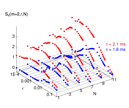
Figure 6: Multiscale entropy $S_{E}$ depending on scale factor $N$ and box size $r$. For regular motion we expect the entropy to approach zero with decreasing $r$. For chaotic dynamics the entropy should stay finite. Since $S_{E}$ is not decreasing with scale factor significantly, it seems there is no characteristic time scale present in the data.

In Fig. 6 and 7 we further analyze the scale factor dependence of MSE. The entropic measure is always larger for the chaotic time series since it is the more complex one. MSE for small scale factor, Fig. 7a, indicates that there is no characteristic time scale, comparable to $1\!/\!f$-noise Costa2002 . But for larger scale factors MSE is decaying comparable to Gaussian white noise, Fig. 7b. Thus, even in the chaotic case, there exists a characteristic time scale which is close to the delay time.

(a)

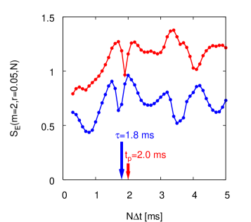
(b)

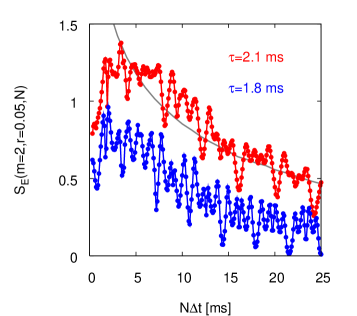
Figure 7: Multiscale entropy $S_{E}$ for fixed $m=2$ and $r=0.05$ depending on scale factor $N$. The time series with delay time $\tau=2.1$ ms seems to be more complex than the time series with delay time $\tau=1.8$ ms since its entropy is larger. a) To gain a higher scale factor resolution we recorded also time series with smaller sampling time $\Delta t=0.1$ ms. b) The existence of a characteristic time scale which is in order of magnitude of the delay time is indicated by the decay of entropy with increasing scale factor $N$. The gray line represents GWN with $r=0.25$.

The frequencies dominating $S(\omega)$, Fig. 3, are also present in $S^{(N)}_{E}(m,r)$. They belong to minima in Fig. 7. We learn coarse-graining of the data over multiple of time scale $t_{p}$ belonging to structures in the cutting process dynamics leads to less complex time series and contains less information.

6 Conclusions and last remarks

Concluding, the 0-1 test differentiates between the two types of motion. Depending on the chosen delay time for the investigated DDE, Eqs. (1) and (2), regular or chaotic motion is observed and a transition from chaotic to regular motion is detected with increasing cutting speed. The nature of solutions has been also confirmed by the corresponding power spectral densities and multiscale entropies. The latter reveals more insights into the process dynamics but is of much higher computational cost than the 0-1 test and the spectral calculations.

The 0-1 test appeared to be relatively simple and, consequently, useful for systems with delay and discontinuities. A huge advantage of the test is its low computational effort and the possibility to compute it ”on the fly” while the data is still growing. One of the useful aspects of the 0-1 test is that the result can be plotted against the parameter $\tau$.

The presented method gives a quantitative criterion for chaos similar to the maximum Lyapunov exponent.

As demonstrated by Falconer et al. Falconer2007 and Krese and Govekar Krese2012 the method can be used on experimental data as well. Unfortunately in case of the cutting process experimental data are often characterized by a relatively high level of noise Litak2004 . In the examined system, we waived the possibility of additive noise. It was shown that the 0-1 test could be applied on dynamical systems with additive noise and a good signal to noise ratio Gottwald2005 .

References

- (1) Taylor, F.: On the art of cutting metals. Trans. ASME 28, 31–350 (1907)
- (2) Arnold, R.N.: The mechanism of tool vibration in the cutting of steel. Proc. Inst. Mech. Eng. 154, 261–284 (1946)
- (3) Tobias, S.A., Fishwick, W.: A Theory of Regenerative Chatter. The Engineer, London (1958)
- (4) Tlusty, J., Polacek, M.: The stability of machine tool against self-excited vibrations in machining. ASME Int. Res. Prod. Eng. 465–474 (1963)
- (5) Merrit, H.E.: Theory of self-excited machine-tool chatter. ASME J. Eng. Ind. 87, 447–454 (1965)
- (6) Wu, D.W., Liu, C.R.: An analytical model of cutting dynamics. Part 1: Model building. ASME J. Eng. Ind. 107, 107–111 (1985)
- (7) Wu, D.W., Liu, C.R.: An analytical model of cutting dynamics. Part 2: Verification. ASME J. Eng. Ind. 107, 112–118 (1985)
- (8) Altintas, Y.: Manufacturing Automation: Metal Cutting Mechanics, Machine Tool Vibrations, and CNC Design. Cambridge University Press, Cambridge (2000)
- (9) Warminski, J., Litak, G., Cartmell M.P., Khanin R., Wiercigroch W.: Approximate analytical solutions for primary chatter in the nonlinear metal cutting model. J. Sound Vibr. 259, 917–933 (2003)
- (10) Insperger, T., Gradisek, J., Kalveram, M., Stépán, G., Winert K., Govekar E.: Machine tool chatter and surface location error in milling processes. J. Manufac. Sci. Eng. 128, 913–920 (2006)
- (11) Ganguli, A., Deraemaeker, A., Preumont, A.: Regenerative chatter reduction by active damping control. J. Sound Vibr. 300, 847–862 (2007)
- (12) Grabec I.: Chaotic dynamics of the cutting process. Int. J. Mach. Tools Manuf. 28, 19–32 (1988)
- (13) Tansel, I.N., Erkal, C., Keramidas, T.: The chaotic characteristics of three-dimensional cutting. Int. J. Mach. Tools Manufact. 32, 811–827 (1992)
- (14) Gradisek, J., Govekar E., Grabec, I.: Time series analysis in metal cutting: chatter versus chatter-free cutting. Mech. Syst. Signal Process 12, 839–854 (1998)
- (15) Gradisek, J., Govekar, E., Grabec I.: Using coarse-grained entropy rate to detect chatter in cutting. J. Sound Vibr. 214, 941–952 (1998)
- (16) Marghitu, D.B., Ciocirlan, B.O., Craciunoiu, N.: Dynamics in orthogonal turning process. Chaos, Solitons & Fractals 12, 2343–2352 (2001)
- (17) Litak G.: Chaotic vibrations in a regenerative cutting process. Chaos, Solitons & Fractals 13, 1531–1535 (2002)
- (18) Fofana, M.S.: Delay dynamical systems and applications to nonlinear machine-tool chatter. Chaos, Solitons & Fractals 12 731–747 (2003)
- (19) Gradisek, J., Grabec, I., Sigert, I., Friedrich, R.: Stochastic dynamics of metal cutting: bifurcation phenomena in turning. Mech. Syst. Signal Process. 16, 831–840 (2002)
- (20) Litak, G., Rusinek, R., Teter A.: Nonlinear analysis of experimental time series of a straight turning process. Meccanica 39, 105–112 (2004)
- (21) Stépán, G., Szalai, R., Insperger, T.: Nonlinear dynamics of high-speed milling subjected to regenerative effect. In: Radons, G. (ed.): Nonlinear Dynamics of Production Systems. Wiley, New York (2003)
- (22) Vela-Martínez, L., Jáuregui-Correa, J.C., González-Brambila, O.M., Herrera-Ruiz, G., Lozano-Guzmán, A.: Instability conditions due to structural nonlinearities in regenerative chatter. Nonlinear Dynamics 56, 415–427 (2009)
- (23) Gottwald G.A., Melbourne, I.: A new test for chaos in deterministic systems. Proc. R. Soc. Lond. A 460, 603–611 (2004)
- (24) Gottwald G.A., Melbourne, I.: Testing for chaos in deterministic systems with noise. Physica D 212, 100–110 (2005)
- (25) Falconer, I., Gottwald, G.A., Melbourne, I., Wormnes, K.: Application of the 0-1 test for chaos to experimental data. SIAM J. App. Dyn. Syst. 6, 95-402 (2007)
- (26) Gottwald, G.A., Melbourne, I.: On the implementation of the 0-1 test for chaos. SIAM J. App. Dyn. Syst. 8, 129-145 (2009)
- (27) Gottwald, G.A., Melbourne, I.: On the validity of the 0-1 test for chaos. Nonlinearity 22, 1367–1382 (2009)
- (28) Litak, G., Syta, A., Wiercigroch, M.: Identification of chaos in a cutting process by the 0-1 test. Chaos, Solitons & Fractals 40, 2095–2101 (2009)
- (29) Pratt, J.R., Nayfeh, A.H.: Chatter control and stability analysis of a cantilever boring bar under regenerative cutting conditions. Philos. Trans. R. Soc. Lond. A 359, 759–792 (2001)
- (30) Stépán, G.: Modelling nonlinear regenerative effects in metal cutting. Philos. Trans. R. Soc. Lond. A 359, 739–757 (2001)
- (31) Wang X.S., Hu, J., Gao, J.B.: Nonlinear dynamics of regenerative cutting processes – Comparison of two models. Chaos, Solitons & Fractals 29, 1219–1228 (2006)
- (32) Litak, G., Sen A.K., Syta, A.: Intermittent and chaotic vibrations in a regenerative cutting process. Chaos, Solitons & Fractals 41, 2115–2122 (2009)
- (33) Krese, B., Govekar, E.: Nonlinear analysis of laser droplet generation by means of 0-1 test for chaos. Nonlinear Dynamics 67, 2101-–2109 (2012)
- (34) Costa, M., Goldberger, A.L., Peng, C.-K.: Multiscale analysis of complex biological signals. Phys. Rev. Lett. 89, 068102 (2002)
- (35) Costa, M., Goldberger, A.L., Peng, C.-K.: Multiscale analysis of biological signals. Phys. Rev. E 89, 021906 (2005)
- (36) Goldberger, A.L., Amaral, L.A.N., Glass, L., Hausdorff, J.M., Ivanov, P.Ch., Mark, R.G., Mietus, J.E., Moody, G.B., Peng, C.-K., Stanley, H.E.: PhysioBank, physioToolkit, and physioNet: Components of a new research resource for complex physiologic signals. Circulation 101, 215–220 (2000)
- (37) Richman, J.S, Moorman, J.R.: Physiological time-series analysis using approximate entropy and sample entropy. Am. J. Physiol. 278, H2039–H2049 (2000)
- (38) Grassberger, P., Procaccia, I.: Estimation of the Kolmogorov-entropy from a chaotic signal. Phys. Rev. A 28, 2591-2593 (1983)