Maximal stream and minimal cutset for first passage percolation through a domain of $\mathbb{R}$^d

Abstract

We consider the standard first passage percolation model in the rescaled graph $\mathbb{Z}^{d}/n$ for $d\geq 2$ and a domain $\Omega$ of boundary $\Gamma$ in $\mathbb{R}^{d}$. Let $\Gamma^{1}$ and $\Gamma^{2}$ be two disjoint open subsets of $\Gamma$, representing the parts of $\Gamma$ through which some water can enter and escape from $\Omega$. A law of large numbers for the maximal flow from $\Gamma^{1}$ to $\Gamma^{2}$ in $\Omega$ is already known. In this paper we investigate the asymptotic behavior of a maximal stream and a minimal cutset. A maximal stream is a vector measure $\vec{\mu}_{n}^{\max}$ that describes how the maximal amount of fluid can cross $\Omega$. Under conditions on the regularity of the domain and on the law of the capacities of the edges, we prove that the sequence $(\vec{\mu}_{n}^{\max})_{n\geq 1}$ converges a.s. to the set of the solutions of a continuous deterministic problem of maximal stream in an anisotropic network. A minimal cutset can been seen as the boundary of a set $E_{n}^{\min}$ that separates $\Gamma^{1}$ from $\Gamma^{2}$ in $\Omega$ and whose random capacity is minimal. Under the same conditions, we prove that the sequence $(E_{n}^{\min})_{n\geq 1}$ converges toward the set of the solutions of a continuous deterministic problem of minimal cutset. We deduce from this a continuous deterministic max-flow min-cut theorem and a new proof of the law of large numbers for the maximal flow. This proof is more natural than the existing one, since it relies on the study of maximal streams and minimal cutsets, which are the pertinent objects to look at.

Maximal stream and minimal cutset for first passage percolation through a domain of Rd

and

60K35, 49K20, 35Q35, 82B20, First passage percolation, continuous and discrete max-flow min-cut theorem, maximal stream, maximal flow

1 First definitions and main result

We recall first the definitions of the random discrete model and of the discrete objects. The continuous counterparts of the discrete objects are briefly presented in Section 1.2 and the main results are presented in Section 1.3.

1.1 Discrete streams, cutsets and flows

We use many notation introduced in Kesten:StFlour and Kesten:flows . Let $d\geq 2$. We consider the graph $(\mathbb{Z}^{d}_{n},\mathbb{E}^{d}_{n})$ having for vertices $\mathbb{Z}^{d}_{n}=\mathbb{Z}^{d}/n$ and for edges $\mathbb{E}^{d}_{n}$, the set of pairs of nearest neighbors for the standard $L^{1}$ norm. With each edge $e$ in $\mathbb{E}^{d}_{n}$ we associate a random variable $t(e)$ with values in $\mathbb{R}^{+}$. We suppose that the family $(t(e),e\in\mathbb{E}^{d}_{n})$ is independent and identically distributed, with a common law $\Lambda$: this is the standard model of first passage percolation on the graph $(\mathbb{Z}^{d}_{n},\mathbb{E}^{d}_{n})$. We interpret $t(e)$ as the capacity of the edge $e$; it means that $t(e)$ is the maximal amount of fluid that can go through the edge $e$ per unit of time.

We consider an open bounded connected subset $\Omega$ of $\mathbb{R}^{d}$ such that the boundary $\Gamma=\partial\Omega$ of $\Omega$ is piecewise of class $\mathcal{C}^{1}$. It means that $\Gamma$ is included in the union of a finite number of hypersurfaces of class $\mathcal{C}^{1}$, that is, in the union of a finite number of $\mathcal{C}^{1}$ submanifolds of $\mathbb{R}^{d}$ of codimension $1$. Let $\Gamma^{1}$, $\Gamma^{2}$ be two disjoint subsets of $\Gamma$ that are open in $\Gamma$. We want to study the maximal streams from $\Gamma^{1}$ to $\Gamma^{2}$ through $\Omega$ for the capacities $(t(e),e\in\mathbb{E}^{d}_{n})$. We consider a discrete version $(\Omega_{n},\Gamma_{n},\Gamma^{1}_{n},\Gamma^{2}_{n})$ of $(\Omega,\Gamma,\Gamma^{1},\Gamma^{2})$ defined by

$$\cases{\Omega_{n}=\bigl{\{}x\in\mathbb{Z}^{d}_{n}|d_{\infty}(x,\Omega)<1/n\bigr{\}},\vspace*{2pt}\cr\Gamma_{n}=\bigl{\{}x\in\Omega_{n}|\exists y\notin\Omega_{n},[x,y]\in\mathbb{E}^{d}_{n}\bigr{\}},\vspace*{2pt}\cr\Gamma^{i}_{n}=\bigl{\{}x\in\Gamma_{n}|d_{\infty}\bigl{(}x,\Gamma^{i}\bigr{)}<1/n,d_{\infty}\bigl{(}x,\Gamma^{3-i}\bigr{)}\geq 1/n\bigr{\}},&\quad$\mbox{ for }i=1,2,$}$$

where $d_{\infty}$ is the $L^{\infty}$-distance, and the segment $[x,y]$ is the edge of endpoints $x$ and $y$; see Figure 1. We denote by $\Pi_{n}$ the set of the edges with both endpoints in $\Omega_{n}$.

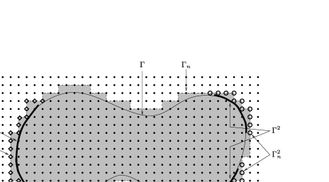
Figure 1: Domain $\Omega$.

We shall study streams and flows from $\Gamma^{1}_{n}$ to $\Gamma^{2}_{n}$ and cutsets between $\Gamma^{1}_{n}$ and $\Gamma^{2}_{n}$ in $\Omega_{n}$. Let us define first the admissible streams from $F_{1}$ to $F_{2}$ in $C$, for $C$ a bounded connected subset of $\mathbb{R}^{d}$ and $F_{1},F_{2}$ disjoint sets of vertices of $\mathbb{Z}^{d}_{n}$ included in $C$. We will say that an edge $e=[x,y]$ is included in a subset $A$ of $\mathbb{R}^{d}$, which we denote by $e\subset A$, if the closed segment joining $x$ to $y$ is included in $A$. Let $e=[a,b]$ be an edge of $\mathbb{E}^{d}_{n}$ with endpoints $a$ and $b$. We denote by $\langle a,b\rangle$ the oriented edge starting at $a$ and ending at $b$. We fix next an orientation for each edge of $\mathbb{E}^{d}_{n}$. Let $(\vec{\mathbf{f}}_{1},\ldots,\vec{\mathbf{f}}_{n})$ be the canonical basis of $\mathbb{R}^{d}$. We denote by $\mathbb{E}_{n}^{d,i}$ the set of the edges parallel to $\vec{\mathbf{f}}_{i}$. For $e=[a,b]\in\mathbb{E}^{d,i}_{n}$, we define

$$\vec{e}=\vec{\mathbf{f}}_{i}\quad\mbox{and}\quad\mathbf{e}=\cases{\langle a,b\rangle,&\quad$\mbox{if }\overrightarrow{ab}\cdot\vec{\mathbf{f}}_{i}=+1/n,$\vspace*{2pt}\cr\langle b,a\rangle,&\quad$\mbox{if }\overrightarrow{ab}\cdot\vec{\mathbf{f}}_{i}=-1/n,$}$$

where $\cdot$ is the scalar product on $\mathbb{R}^{d}$ and $\overrightarrow{ab}$ the vector of origin $a$ and endpoint $b$. We define the set $\mathcal{S}_{n}(F_{1},F_{2},C)$ of admissible “stream functions” as the set of functions $f_{n}\dvtx\mathbb{E}^{d}_{n}\rightarrow\mathbb{R}$ such that: [(iii)]

the stream is inside $C$: for each edge $e\not\subset C$ we have $f_{n}(e)=0$;

capacity constraint: for each edge $e\in\mathbb{E}^{d}_{n}$ we have

$$\bigl{|}f_{n}(e)\bigr{|}\leq t(e);$$

conservation law: for each vertex $v\in\mathbb{Z}^{d}_{n}\setminus(F_{1}\cup F_{2})$ we have

$$\sum_{e\in\mathbb{E}^{d}_{n}:\mathbf{e}=\langle v,\cdot\rangle}f_{n}(e)=\sum_{e\in\mathbb{E}^{d}_{n}:\mathbf{e}=\langle\cdot,v\rangle}f_{n}(e),$$

where the notation $\mathbf{e}=\langle v,\cdot\rangle$ (resp., $\mathbf{e}=\langle\cdot,v\rangle$) means that there exists $y\in\mathbb{Z}_{n}^{d}$ such that $\mathbf{e}=\langle v,y\rangle$ (resp., $\mathbf{e}=\langle y,v\rangle$). A function $f_{n}\in\mathcal{S}_{n}(F_{1},F_{2},C)$ is a description of a possible stream in $C$: $|f_{n}(e)|$ is the amount of water that crosses $e$ per second, and this water goes through $e$ in the direction of $f_{n}(e)\mathbf{e}$ (thus in the direction of $\mathbf{e}$ is $f_{n}(e)>0$ and in the direction of $-\mathbf{e}$ if $f_{n}(e)<0$). Condition (i) means that the water does not move outside $C$; condition (ii) means that the amount of water that can cross $e$ per second cannot exceed $t(e)$; condition (iii) means that there is no loss of fluid in the graph. To each stream function $f_{n}$ from $F_{1}$ to $F_{2}$ in $C$, we associate the corresponding flow

$$\operatorname{flow}^{\mathrm{disc}}_{n}(f_{n})=\sum_{e\subset C:e=[a,b],a\in F_{1},b\notin F_{1}}f_{n}(e)(\mathbh{1}_{\{\mathbf{e}=\langle a,b\rangle\}}-\mathbh{1}_{\{\mathbf{e}=\langle b,a\rangle\}}).$$

This is the amount of fluid (positive or negative) that crosses $C$ from $F_{1}$ to $F_{2}$ according to $f_{n}$. We define the maximal flow $\phi_{n}(F_{1},F_{2},C)$ from $F_{1}$ to $F_{2}$ in $C$ by

$$\phi_{n}(F_{1},F_{2},C)=\sup\bigl{\{}\operatorname{flow}^{\mathrm{disc}}_{n}(f_{n})|f_{n}\in\mathcal{S}_{n}(F_{1},F_{2},C)\bigr{\}}.$$

If $D$ is a connected set of vertices of $\mathbb{Z}^{d}_{n}$ that contains two disjoint subsets $F_{1},F_{2}$ of $\mathbb{Z}^{d}_{n}$, we define

$$\widehat{D}=D+\frac{1}{2n}[-1,1]^{d}\subset\mathbb{R}^{d}.$$

We define

$$\mathcal{S}_{n}(F_{1},F_{2},D)=\mathcal{S}_{n}(F_{1},F_{2},\widehat{D})\quad\mbox{and}\quad\phi_{n}(F_{1},F_{2},D)=\phi_{n}(F_{1},F_{2},\widehat{D}).$$

The maximal flow $\phi_{n}(F_{1},F_{2},C)$ can be expressed differently thanks to the (discrete) max-flow min-cut theorem; see Bollobas . We need some definitions to state this result. A path on the graph $\mathbb{Z}_{n}^{d}$ from the vertex $v_{0}$ to the vertex $v_{m}$ is a sequence $(v_{0},e_{1},v_{1},\ldots,e_{m},v_{m})$ of vertices $v_{0},\ldots,v_{m}$ alternating with edges $e_{1},\ldots,e_{m}$ such that $v_{i-1}$ and $v_{i}$ are neighbors in the graph, joined by the edge $e_{i}$, for $i$ in $\{1,\ldots,m\}$. A set $E$ of edges of $\mathbb{E}^{d}_{n}$ included in $C$ is said to cut $F_{1}$ from $F_{2}$ in $C$ if there is no path from $F_{1}$ to $F_{2}$ made of edges included in $C$ that do not belong to $E$. We call $E$ an $(F_{1},F_{2})$-cutset in $C$ if $E$ cuts $F_{1}$ from $F_{2}$ in $C$ and if no proper subset of $E$ does. With each set of edges $E\subset\mathbb{E}^{d}_{n}$ we associate its capacity which is the random variable

$$V(E)=\sum_{e\in E}t(e).$$

The max-flow min-cut theorem states that

$$\phi_{n}(F_{1},F_{2},C)=\min\bigl{\{}V(E)|E\subset\mathbb{E}^{d}_{n}\mbox{ is a }(F_{1},F_{2})\mbox{-cutset in }C\bigr{\}}.$$

We can achieve a better understanding of what a cutset is thanks to the following correspondence. We associate to each edge $e\in\mathbb{E}^{d,i}_{n}$ a plaquette $\pi(e)$ defined by

$$\pi(e)=c(e)+\frac{1}{2n}\bigl{(}[-1,1]^{i-1}\times\{0\}\times[-1,1]^{d-i}\bigr{)},$$

where $c(e)$ is the middle of the edge $e$. To a set of edges $E\subset\mathbb{E}^{d}_{n}$ we associate the set of the corresponding plaquettes $E^{*}=\bigcup_{e\in E}\pi(e)$. If $E$ is a $(F_{1},F_{2})$-cutset, then $E^{*}$ looks like a “surface” of plaquettes that separates $F_{1}$ from $F_{2}$ in $C$; see Figure 2. We do not try to give a proper definition to the term “surface” appearing here. In terms of plaquettes, the discrete max-flow min-cut theorem states that the maximal flow from $F_{1}$ to $F_{2}$ in $C$, given a local constraint on the maximal amount of water that can cross each edge, is equal to the minimal capacity of a “surface” that cuts $F_{1}$ from $F_{2}$ in $C$.

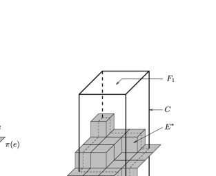
Figure 2: Set of plaquettes $E^{*}$ corresponding to a $(F_{1},F_{2})$-cutset $E$ in $C$.

We consider now streams, cutsets and flows in $\Omega_{n}$. The set of stream functions associated to our flow problem is $\mathcal{S}_{n}(\Gamma^{1}_{n},\Gamma^{2}_{n},\Omega_{n})$. We will denote by $\phi_{n}$ the maximal flow $\phi_{n}(\Gamma^{1}_{n},\Gamma^{2}_{n},\Omega_{n})$. To each $f_{n}\in\mathcal{S}_{n}(\Gamma^{1}_{n},\Gamma^{2}_{n},\Omega_{n})$, we associate the vector measure $\vec{\mu}_{n}$, that we call the stream itself, defined by

$$\vec{\mu}_{n}=\vec{\mu}_{n}(f_{n})=\frac{1}{n^{d}}\sum_{e\in\mathbb{E}^{d}_{n}}f_{n}(e)\vec{e}\delta_{c(e)},$$

where $c(e)$ is the center of $e$. Notice that since $f_{n}\in\mathcal{S}_{n}(\Gamma^{1}_{n},\Gamma^{2}_{n},\Omega_{n})$, the condition (i) implies that $f_{n}(e)=0$ for all $e\notin\Pi_{n}$; thus the sum in the previous definition is finite. A stream $\vec{\mu}_{n}$ is a rescaled measure version of a stream function $f_{n}$. The vector measure $\vec{\mu}_{n}$ is defined on $(\mathbb{R}^{d},\mathcal{B}(\mathbb{R}^{d}))$ where $\mathcal{B}(\mathbb{R}^{d})$ is the collection of the Borel sets of $\mathbb{R}^{d}$ and takes values in $\mathbb{R}^{d}$. In fact $\vec{\mu}_{n}=(\mu_{n}^{1},\ldots,\mu_{n}^{d})$ where $\mu_{n}^{i}$ is a signed measure on $(\mathbb{R}^{d},\mathcal{B}(\mathbb{R}^{d}))$ for all $i\in\{1,\ldots,d\}$. We define the flow corresponding to a stream $\vec{\mu}_{n}(f_{n})$ as $\operatorname{flow}^{\mathrm{disc}}_{n}(f_{n})$ properly rescaled,

$$\operatorname{flow}^{\mathrm{disc}}_{n}(\vec{\mu}_{n})=\operatorname{flow}^{\mathrm{disc}}_{n}\bigl{(}\vec{\mu}_{n}(f_{n})\bigr{)}=\frac{1}{n^{d-1}}\operatorname{flow}^{\mathrm{disc}}_{n}(f_{n}).$$

We say that $\vec{\mu}_{n}=\vec{\mu}_{n}(f_{n})$ is a maximal stream from $\Gamma^{1}_{n}$ to $\Gamma^{2}_{n}$ in $\Omega_{n}$ if and only if

$$\operatorname{flow}^{\mathrm{disc}}_{n}(\vec{\mu}_{n})=\frac{\phi_{n}}{n^{d-1}},$$ (1)

and for any $e=[a,b]$ such that $a\in\Gamma^{1}_{n}$ and $b\notin\Gamma^{1}_{n}$, we have $f_{n}(e)\vec{e}\cdot\overrightarrow{ab}\geq 0$, that is,

$$f_{n}(e)\cases{\geq 0,&\quad$\mbox{if }\mathbf{e}\mbox{ is oriented from }a\mbox{ to }b\ \bigl{(}\mbox{i.e. }\mathbf{e}=\langle a,b\rangle\bigr{)},$\vspace*{2pt}\cr\leq 0,&\quad$\mbox{if }\mathbf{e}\mbox{ is oriented from }b\mbox{ to }a\ \bigl{(}\mbox{i.e. }\mathbf{e}=\langle b,a\rangle\bigr{)}.$}$$ (2)

The set of admissible stream functions is random since the capacity constraint on the stream is random. Thus $\phi_{n}$ is random and the set of admissible streams (resp., maximal streams) from $\Gamma^{1}_{n}$ to $\Gamma^{2}_{n}$ in $\Omega_{n}$ is random too.

Let $\mathcal{E}_{n}$ be a $(\Gamma^{1}_{n},\Gamma^{2}_{n})$-cutset in $\Omega_{n}$. We say that $\mathcal{E}_{n}$ is a minimal cutset if and only if it realizes the minimum

$$V(\mathcal{E}_{n})=\phi_{n}$$ (3)

and it has minimal cardinality, that is,

$$\operatorname{card}(\mathcal{E}_{n})=\min\bigl{\{}\operatorname{card}(\mathcal{F}_{n})|\mathcal{F}_{n}\mbox{ is a }\bigl{(}\Gamma^{1}_{n},\Gamma^{2}_{n}\bigr{)}\mbox{-cutset in }\Omega_{n}\mbox{ and}$$

(4)

$$\hskip 130.0pt\qquad V(\mathcal{F}_{n})=\phi_{n}\bigl{(}\Gamma^{1}_{n},\Gamma^{2}_{n},\Omega_{n}\bigr{)}\bigr{\}},$$

where $\operatorname{card}(\mathcal{E})$ denotes the cardinality of the set $\mathcal{E}$. We want to see a cutset $\mathcal{E}_{n}$ as the “boundary” of a subset of $\Omega$. We define the set $r(\mathcal{E}_{n})\subset\mathbb{Z}^{d}_{n}$ by

$$r(\mathcal{E}_{n})=\bigl{\{}x\in\Omega_{n}|\mbox{there exists a path from }x\mbox{ to }\Gamma^{1}_{n}\mbox{ in }\bigl{(}\mathbb{Z}^{d}_{n},\Pi_{n}\setminus\mathcal{E}_{n}\bigr{)}\bigr{\}}.$$

Then the edge boundary $\partial^{e}r(\mathcal{E}_{n})$ of $r(\mathcal{E}_{n})$, defined by

$$\partial^{e}r(\mathcal{E}_{n})=\bigl{\{}e=[x,y]\in\Pi_{n}|x\in r(\mathcal{E}_{n})\mbox{ and }y\notin r(\mathcal{E}_{n})\bigr{\}},$$

is exactly equal to $\mathcal{E}_{n}$. We consider a “non discrete version” $R(\mathcal{E}_{n})$ of $r(\mathcal{E}_{n})$ defined by

$$R(\mathcal{E}_{n})=r(\mathcal{E}_{n})+\frac{1}{2n}[-1,1]^{d}.$$

Notice that $\mathcal{E}_{n}=\partial^{e}(R(\mathcal{E}_{n})\cap\Pi_{n})$; thus the sets $\mathcal{E}_{n}$ and $R(\mathcal{E}_{n})$ completely define one each other; see Figure 3.

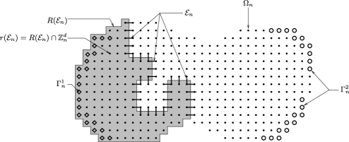
Figure 3: A $(\Gamma^{1}_{n},\Gamma^{2}_{n})$-cutset $\mathcal{E}_{n}$ in $\Omega_{n}$ and the corresponding sets $r(\mathcal{E}_{n})$ and $R(\mathcal{E}_{n})$.

Remark 1.

We want to study the asymptotic behavior of sequences of maximal streams and minimal cutsets. For a fixed $n$ and given capacities, the existence of at least one minimal cutset is obvious since there are finitely many cutsets. The existence of at least one maximal stream is not so obvious because of condition (2). Under the hypothesis that the capacities are bounded, we will prove in Section 4.1 that a maximal stream exists.

1.2 Brief presentation of the limiting objects

We consider a sequence $(\vec{\mu}_{n}^{\max})_{n\geq 1}$ of maximal streams and a sequence $(\mathcal{E}_{n}^{\min})_{n\geq 1}$ of minimal cutsets. For each $n$, $\vec{\mu}_{n}^{\max}$ is a solution of a discrete random problem of maximal flow, $\mathcal{E}_{n}^{\min}$ is a solution of a discrete random problem of minimal cutset and by the max-flow min-cut theorem

$$\operatorname{flow}^{\mathrm{disc}}_{n}\bigl{(}\vec{\mu}_{n}^{\max}\bigr{)}=\frac{V(\mathcal{E}_{n}^{\min})}{n^{d-1}}:=\frac{\phi_{n}}{n^{d-1}},$$

where $\phi_{n}$ stands for $\phi_{n}(\Gamma^{1}_{n},\Gamma^{2}_{n},\Omega_{n})$. The goal of this article is to prove that:

• $(\vec{\mu}_{n}^{\max})_{n\geq 1}$ converges in a way when $n$ goes to infinity to a continuous stream $\vec{\mu}$ which is the solution of a continuous deterministic max-flow problem to be precised;

• $(\mathcal{E}_{n}^{\min})_{n\geq 1}$ converges in a way when $n$ goes to infinity to a continuous cutset $\mathcal{E}$ which is the solution of a continuous deterministic min-cut problem to be precised;

• these continuous deterministic max-flow and min-cut problems are in correspondence, that is, the flow of $\vec{\mu}$ is equal to the capacity of $\mathcal{E}$, and $\phi_{n}/n^{d-1}$ converges toward this constant.

We obtain these results, except that the continuous max-flow and min-cut problems we define may have several solutions, thus we obtain the convergence of the discrete streams $\vec{\mu}_{n}^{\max}$ (resp., the discrete cutsets $\mathcal{E}_{n}^{\min}$) toward the set of the solutions of a continuous deterministic max flow problem (resp., min-cut problem). In this section, we try to present very briefly these continuous max-flow and min-cut problems. A complete and rigorous description will be given in Sections 2.2 and 2.3. The aim of the present section is to give an intuitive idea of the objects involved in the main theorems of Section 1.3.

The first quantity that has been studied is the maximal flow $\phi_{n}$; however, a law of large numbers for $\phi_{n}$ is difficult to establish in a general domain. It is considerably simpler in the following situation. Let $\vec{v}$ be a unit vector in $\mathbb{R}^{d}$, let $Q(\vec{v})$ be a unit cube centered at the origin having two faces orthogonal to $\vec{v}$ and let

$$F_{1}=\{x\in\partial Q|\overrightarrow{0x}\cdot\vec{v}<0\},\qquad F_{2}=\{x\in\partial Q|\overrightarrow{0x}\cdot\vec{v}>0\}$$

be, respectively, the upper half part and the lower half part of the boundary of $Q$ in the direction $\vec{v}$. Whenever $\mathbb{E}(t(e))<\infty$, a subadditive argument yields the following convergence:

$$\lim_{n\rightarrow\infty}\frac{\phi_{n}(F_{1},F_{2},Q(\vec{v}))}{n^{d-1}}=\nu(\vec{v})\qquad\mbox{in }L^{1},$$ (5)

where $\nu(\vec{v})$ is deterministic and depends on the law of the capacities of the edges, the dimension and $\vec{v}$. The maximal flow considered here is not well defined, since $F_{1}$ and $F_{2}$ are not sets of vertices (a rigorous definition will be given in Section 2.3), but equation (5) allows us to understand what the constant $\nu(\vec{v})$ represents. By the max-flow min-cut theorem, $\phi_{n}(F_{1},F_{2},Q(\vec{v}))$ is the minimal capacity of a “surface” of plaquettes that cuts $F_{1}$ from $F_{2}$ in $Q(\vec{v})$, thus a discrete “surface” whose boundary is spanned by $\partial Q(\vec{v})$. Thus the constant $\nu(\vec{v})$ can be seen as the average asymptotic capacity of a continuous unit surface normal to $\vec{v}$. By symmetry we have $\nu(\vec{v})=\nu(-\vec{v})$.

This interpretation of $\nu(\vec{v})$ provides in a natural way the desired continuous deterministic min-cut problem. Indeed, if $\mathcal{S}$ is a “nice” surface (“nice” means $\mathcal{C}^{1}$ among other things), it is natural to define its capacity as

$$\operatorname{capacity}(\mathcal{S})=\int_{\mathcal{S}\cap\Omega}\nu\bigl{(}\vec{v}_{\mathcal{S}}(x)\bigr{)}\,d\mathcal{H}^{d-1}(x),$$

where $\mathcal{H}^{d-1}$ is the $(d-1)$-dimensional Hausdorff measure on $\mathbb{R}^{d}$, and $\vec{v}_{\mathcal{S}}(x)$ is a unit vector normal to $\mathcal{S}$ at $x$. Exactly as a discrete cutset $\mathcal{E}_{n}$ can be seen as the boundary of a set $R(\mathcal{E}_{n})$, we see $\mathcal{S}$ as the boundary of a set $F\subset\Omega$, and we define $\operatorname{capacity}(F)=\operatorname{capacity}(\partial F)$. The continuous deterministic min-cut problem we consider is the following:

$$\phi_{\Omega}^{a}:=\inf\bigl{\{}\operatorname{capacity}(F)|F\subset\Omega,\partial F\mbox{ is a surface separating }\Gamma^{1}\mbox{ from }\Gamma^{2}\mbox{ in }\Omega\bigr{\}}.$$

The above variational problem is loosely defined, since we did not give a definition of $\operatorname{capacity}(F)$ for all $F$, and we did not describe precisely the admissible sets $F$: we should precise the regularity required on $\partial F$ and what “separating” means. This will be done in Section 2.3. We will denote by $\Sigma^{a}$ the set of the continuous minimal cutsets, that is,

$$\Sigma^{a}=\bigl{\{}F\subset\Omega|F\mbox{ is ``admissible'' and }\operatorname{capacity}(F)=\phi_{\Omega}^{a}\bigr{\}}.$$

The variational problem $\phi_{\Omega}^{a}$ is a very good candidate to be the continuous min-cut problem we are looking for, all the more since it has been proved by the authors in the companion papers CerfTheret09supc , CerfTheret09geoc and CerfTheret09infc that under suitable hypotheses

$$\lim_{n\rightarrow\infty}\frac{\phi_{n}}{n^{d-1}}=\phi_{\Omega}^{a}\qquad\mbox{a.s.}$$

This result is presented in Section 2.3. By studying maximal streams and minimal cutsets, we will give an alternative proof of this law of large numbers for $\phi_{n}$.

We define now a continuous max-flow problem. A continuous stream in $\Omega$ will be modeled by a vector field $\vec{\sigma}\dvtx\mathbb{R}^{d}\rightarrow\mathbb{R}^{d}$ that must satisfy constraints equivalent to (i), (ii) and (iii). For a “nice” stream $\vec{\sigma}$ (e.g., $\vec{\sigma}$ is $\mathcal{C}^{1}$ on the closure $\overline{\Omega}$ of $\Omega$ and on $\mathbb{R}^{d}\setminus\overline{\Omega}$) these constraints would be: [(iii

$${}^{\prime})]\par\emph{the stream is inside $\Omega$}:\vec{\sigma}=0on\mathbb{R}^{d}\setminus\overline{\Omega};\par\emph{capacity constraint}:\forall\vec{v}\in\SS^{d-1},\vec{\sigma}\cdot\vec{v}\leq\nu(\vec{v})on\mathbb{R}^{d};\par\emph{conservation law}:\operatorname{div}\vec{\sigma}=0on\Omega and\vec{\sigma}\cdot\vec{v}_{\Omega}=0on\Gamma\setminus(\Gamma^{1}\cup\Gamma^{2}).Here\SS^{d-1}istheunitsphereof\mathbb{R}^{d}and\vec{v}_{\Omega}(x)denotestheexteriorunitvectornormalto\Omega atx.Theflowcorrespondingtoa``nice^{\prime\prime}stream\vec{\sigma}wouldbe$$\operatorname{flow}^{\mathrm{cont}}(\vec{\sigma})=\int_{\Gamma^{1}}-\vec{\sigma}\cdot\vec{v}_{\Omega}\,d\mathcal{H}^{d-1}.$$Thusweobtainthefollowingcontinuousmax-flowproblem:$$\phi_{\Omega}^{b}:=\sup\left\{\operatorname{flow}^{\mathrm{cont}}(\vec{\sigma})\left|\begin{array}[]{l}\vec{\sigma}\dvtx\mathbb{R}^{d}\rightarrow\mathbb{R}^{d}\mbox{ is a stream inside }\Omega\mbox{ that satisfies}\\ \mbox{the capacity constraint and the conservation law}\end{array}\right.\right\}.$$Theabovevariationalproblemislooselydefinedtoo,sincewedidnotgiveadefinitionof\operatorname{flow}^{\mathrm{cont}}(\vec{\sigma})forall\vec{\sigma},andwedidnotdescribepreciselythesetofadmissiblestreams\vec{\sigma}:weshouldprecisetheregularityrequiredon\vec{\sigma}andadaptconditions~{}(i^{\prime}),(ii^{\prime})and(iii^{\prime})to\vec{\sigma}inthisclassofregularity.ThiswillbedoneinSection~{}\ref{secNozawa}.Wewilldenoteby\Sigma^{b}thesetofthecontinuousmaximalstreams,thatis,$$\Sigma^{b}=\bigl{\{}\vec{\sigma}\dvtx\mathbb{R}^{d}\rightarrow\mathbb{R}^{d}|\vec{\sigma}\mbox{ is ``admissible'' and }\operatorname{flow}^{\mathrm{cont}}(\vec{\sigma})=\phi_{\Omega}^{b}\bigr{\}}.$$\par\par Wehavealsogoodreasonsaprioritothinkthatthevariationalproblem\phi_{\Omega}^{b}isthemax-flowproblemwearelookingfor.Indeed,variouscontinuousversionsofthemax-flowmin-cuttheoremhavebeenproved(see,e.g.,\mbox{\cite[cite]{\@@bibref{Authors Phrase1YearPhrase2}{Blum,Strang,Nozawa}{\@@citephrase{(}}{\@@citephrase{)}}}}),andamainresultofNozawa^{\prime}swork\cite[cite]{\@@bibref{Authors Phrase1YearPhrase2}{Nozawa}{\@@citephrase{(}}{\@@citephrase{)}}}ispreciselytoprovethat$$\phi_{\Omega}^{b}=\phi_{\Omega}^{a^{\prime}},$$where\phi_{\Omega}^{a^{\prime}}isavariantof\phi_{\Omega}^{a}.Thankstoourstudyofmaximalflowsandminimalcutsets,wewillalsorecoverthiscontinuousmax-flowmin-cuttheoreminoursetting.\par\begin{rem}Wegavenoargumentaprioritojustifythatthesets\Sigma^{a}and\Sigma^{b}arenotempty.Thiswillbeaconsequenceofourresultsofconvergence.Thefactthat\Sigma^{b}isnotemptywasalreadyprovedbyNozawain\cite[cite]{\@@bibref{Authors Phrase1YearPhrase2}{Nozawa}{\@@citephrase{(}}{\@@citephrase{)}}}.\end{rem}\par\par\par$$

1.3 Main results

We denote by $\mathcal{L}^{d}$ the Lebesgue measure in $\mathbb{R}^{d}$ and by $\mathcal{C}_{b}(\mathbb{R}^{d},\mathbb{R})$ the set of the continuous bounded functions from $\mathbb{R}^{d}$ to $\mathbb{R}$. We define the distance $\mathfrak{d}$ on the subsets of $\mathbb{R}^{d}$ by

$$\forall E,F\subset\mathbb{R}^{d}\qquad\mathfrak{d}(E,F)=\mathcal{L}^{d}(E\triangle F),$$

where $E\triangle F=(E\setminus F)\cup(F\setminus E)$ is the symmetric difference of $E$ and $F$.

We need some hypotheses on $(\Omega,\Gamma^{1},\Gamma^{2})$. We say that $\Omega$ is a Lipschitz domain if its boundary $\Gamma$ can be locally represented as the graph of a Lipschitz function defined on some open ball of $\mathbb{R}^{d-1}$. We say that two $\mathcal{C}^{1}$ hypersurfaces $\mathcal{S}_{1},\mathcal{S}_{2}$ intersect transversally if for all $x\in\mathcal{S}_{1}\cap\mathcal{S}_{2}$, the normal unit vector to $\mathcal{S}_{1}$ and $\mathcal{S}_{2}$ at $x$ are not colinear. We gather here the hypotheses we will make on $(\Omega,\Gamma^{1},\Gamma^{2})$

Hypothesis (H1)

We suppose that $\Omega$ is a bounded open connected subset of $\mathbb{R}^{d}$, that it is a Lipschitz domain and that $\Gamma$ is included in the union of a finite number of oriented hypersurfaces of class $\mathcal{C}^{1}$ that intersect each other transversally; we also suppose that $\Gamma^{1}$ and $\Gamma^{2}$ are open subsets of $\Gamma$, that $\inf\{\|x-y\|,x\in\Gamma^{1},y\in\Gamma^{2})>0$, and that their relative boundaries $\partial_{\Gamma}\Gamma^{1}$ and $\partial_{\Gamma}\Gamma^{2}$ have null $\mathcal{H}^{d-1}$ measure.

We also make the following hypotheses on the law of the capacities:

Hypothesis (H2)

We suppose that the capacities of the edges are bounded by a constant $M$, that is,

$$\exists M<+\infty,\qquad\Lambda\bigl{(}[0,M]\bigr{)}=1.$$

Hypothesis (H3)

We suppose that

$$\Lambda\bigl{(}\{0\}\bigr{)}<1-p_{c}(d),$$

where $p_{c}(d)$ is the critical parameter of edge Bernoulli percolation on $(\mathbb{Z}^{d},\mathbb{E}^{d})$.

We can now state our main results:

Theorem 1.1 ((Law of large numbers for the maximal streams))

We suppose that the hypotheses (H1) and (H2) are fulfilled. For all $n\geq 1$, let $\vec{\mu}_{n}^{\max}$ be a random maximal discrete stream from $\Gamma^{1}_{n}$ to $\Gamma^{2}_{n}$ in $\Omega_{n}$. Then $(\vec{\mu}_{n}^{\max})_{n\geq 1}$ converges weakly a.s. toward the set $\Sigma^{b}$, that is,

$$\mbox{a.s.},\forall f\in\mathcal{C}_{b}\bigl{(}\mathbb{R}^{d},\mathbb{R}\bigr{)}\qquad\lim_{n\rightarrow\infty}\inf_{\vec{\sigma}\in\Sigma^{b}}\biggl{\|}\int_{\mathbb{R}^{d}}f\,d\vec{\mu}_{n}^{\max}-\int_{\mathbb{R}^{d}}f\vec{\sigma}\,d\mathcal{L}^{d}\biggr{\|}=0.$$

Theorem 1.2 ((Law of large numbers for the minimal cutsets))

We suppose that the hypotheses (H1), (H2) and (H3) are fulfilled. For all $n\geq 1$, let $\mathcal{E}_{n}^{\min}$ be a minimal $(\Gamma^{1}_{n},\Gamma^{2}_{n})$-cutset in $\Omega_{n}$. Then the sequence $(R(\mathcal{E}_{n}^{\min}))_{n\geq 1}$ converges a.s. for the distance $\mathfrak{d}$ toward the set $\Sigma^{a}$, that is,

$$a.s.,\qquad\lim_{n\rightarrow\infty}\inf_{F\in\Sigma^{a}}\mathfrak{d}\bigl{(}R\bigl{(}\mathcal{E}_{n}^{\min}\bigr{)},F\bigr{)}=0.$$

Remark 3.

As we will see in Section 2.3, condition (H3) is equivalent to $\nu\neq 0$, where $\nu$ is the function defined by equation (5). Thus if (H3) is not satisfied, then $\nu(\vec{v})=0$ for all $\vec{v}$, $\operatorname{capacity}(F)=0$ for every admissible continuous cutset $F$ and the variational problem $\phi_{\Omega}^{a}$ is trivial.

The two previous theorems lead to the following corollary:

Corollary 1

We suppose that hypotheses (H1) and (H2) are fulfilled. If $\Sigma^{b}$ is reduced to a single stream $\vec{\sigma}$, then any sequence of maximal streams $(\vec{\mu}_{n}^{\max})_{n\geq 1}$ converges a.s. weakly to $\vec{\sigma}\mathcal{L}^{d}$. If hypothesis (H3) is also fulfilled and if $\Sigma^{a}$ is reduced to a single set $F$, then for any sequence of minimal cutsets $(\mathcal{E}_{n}^{\min})_{n\geq 1}$, the corresponding sequence $(R(\mathcal{E}_{n}^{\min}))_{n\geq 1}$ converges a.s. for the distance $\mathfrak{d}$ toward $F$.

Remark 4.

We believe that the uniqueness of the maximal stream or the uniqueness of the minimal cutset in the continuous setting may happen, or not, depending on the domain $\Omega$, the sets $\Gamma^{i},i=1,2$ and the function $\nu$ (thus on the law of the capacities $\Lambda$); however we do not handle this question here.

During the proof of Theorem 1.1, we prove the key inequalities to obtain the following lemma:

Lemma 1

We suppose that hypotheses (H1) and (H2) are fulfilled, and we consider the continuous variational problems $\Sigma^{a}$ and $\Sigma^{b}$ associated to the function $\nu\dvtx\SS^{d-1}\rightarrow\mathbb{R}^{+}$. For every admissible continuous stream $\vec{\sigma}$, for every admissible set $F$, we have

$$\operatorname{flow}^{\mathrm{cont}}(\vec{\sigma})\leq\operatorname{capacity}(F).$$

The proof of Theorems 1.1 and 1.2 relies on a compactness argument. Combining this argument, Theorems 1.1, 1.2 and Corollary 1, we obtain the two following theorems:

Theorem 1.3 ((Max-flow min-cut theorem))

We suppose that the hypotheses (H1) and (H2) are fulfilled, and we consider the continuous variational problems $\Sigma^{a}$ and $\Sigma^{b}$ associated to the function $\nu\dvtx\SS^{d-1}\rightarrow\mathbb{R}^{+}$. Then there exists at least an admissible continuous stream $\vec{\sigma}$ such that $\phi_{\Omega}^{b}=\operatorname{flow}^{\mathrm{cont}}(\vec{\sigma})$, there exists at least an admissible set $F$ such that $\phi_{\Omega}^{a}=\operatorname{capacity}(F)$, and we have the following max-flow min-cut theorem:

$$\phi_{\Omega}^{a}=\phi_{\Omega}^{b}:=\phi_{\Omega}.$$

Theorem 1.4 ((Law of large numbers for the maximal flows))

Suppose that hypotheses (H1) and (H2) are fulfilled. Then we have

$$\lim_{n\rightarrow\infty}\frac{\phi_{n}}{n^{d-1}}=\phi_{\Omega}\qquad\mbox{a.s.}$$

Remark 5.

As will be explained in the next section, the last two theorems do not state new results, since the continuous max-flow min-cut theorem we obtain is a particular case of the one studied by Nozawa in Nozawa , and the law of large numbers for the maximal flows has been proved by the authors in CerfTheret09supc , CerfTheret09geoc , CerfTheret09infc under a weaker assumption on $\Lambda$. However, these results are recovered here by new methods, which are more natural. Indeed, the law of large numbers for $\phi_{n}$ was proved in CerfTheret09supc , CerfTheret09geoc , CerfTheret09infc by a study of its lower and upper large deviations around $\phi_{\Omega}$. The study of the upper large deviations CerfTheret09supc is replaced here by the study of a sequence of maximal streams, which is the most original part of this article and gives a better understanding of the model. The study of the lower large deviations CerfTheret09infc is replaced by the study of a sequence minimal cutsets. The techniques are the same in both cases, but we change our point of view. To conclude, we use in both proofs the result of polyhedral approximation presented in CerfTheret09geoc .

2 Background

We present now the mathematical background on which our work relies. It is the occasion to give a proper description of the variational problems involved in our theorems.

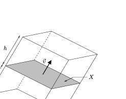
Figure 4: Cylinder $\operatorname{cyl}(X,h)$.

2.1 Some geometric tools

We start with simple geometric definitions. For a subset $X$ of $\mathbb{R}^{d}$, we denote by $\overline{X}$ the closure of $X$, by $\stackrel{{\scriptstyle\circ}}{{X}}$ the interior of $X$, by $X^{c}$ the set $\mathbb{R}^{d}\setminus X$ and by $\mathcal{H}^{s}(X)$ the $s$-dimensional Hausdorff measure of $X$. The $r$-neighborhood $\mathcal{V}_{i}(X,r)$ of $X$ for the distance $d_{i}$, that can be the Euclidean distance if $i=2$ or the $L^{\infty}$-distance if $i=\infty$, is defined by

$$\mathcal{V}_{i}(X,r)=\bigl{\{}y\in\mathbb{R}^{d}|d_{i}(y,X)<r\bigr{\}}.$$

If $X$ is a subset of $\mathbb{R}^{d}$ included in an hyperplane of $\mathbb{R}^{d}$ and of codimension $1$ (e.g., a nondegenerate hyperrectangle), we denote by $\operatorname{hyp}(X)$ the hyperplane spanned by $X$, and we denote by $\operatorname{cyl}(X,h)$ the cylinder of basis $X$ and of height $2h$ defined by

$$\operatorname{cyl}(X,h)=\bigl{\{}x+t\vec{v}|x\in X,t\in[-h,h]\bigr{\}},$$

where $\vec{v}$ is one of the two unit vectors orthogonal to $\operatorname{hyp}(X)$ (see Figure 4). For $x\in\mathbb{R}^{d}$, $r\geq 0$ and a unit vector $\vec{v}$, we denote by $B(x,r)$ the closed ball centered at $x$ of radius $r$, by $\operatorname{disc}(x,r,\vec{v})$ the closed disc centered at $x$ of radius $r$ and normal vector $v$, and by $B^{+}(x,r,\vec{v})$ [resp., $B^{-}(x,r,\vec{v})$] the upper (resp., lower) half part of $B(x,r)$ where the direction is determined by $v$ (see Figure 5), that is,

$$B^{+}(x,r,\vec{v}) = \bigl{\{}y\in B(x,r)|\overrightarrow{xy}\cdot\vec{v}\geq 0\bigr{\}},$$

$$B^{-}(x,r,\vec{v}) = \bigl{\{}y\in B(x,r)|\overrightarrow{xy}\cdot\vec{v}\leq 0\bigr{\}}.$$

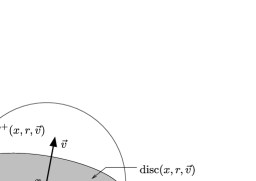
Figure 5: Ball $B(x,r)$.

We denote by $\alpha_{p}$ the volume of the unit ball in $\mathbb{R}^{p}$, $p\geq 1$. Thus $\alpha_{d}$ is the volume of a unit ball in $\mathbb{R}^{d}$, and $\alpha_{d-1}$ the $\mathcal{H}^{d-1}$ measure of a unit disc in $\mathbb{R}^{d}$. We say that a domain $\Omega$ of $\mathbb{R}^{d}$ has Lipschitz boundary if its boundary can be locally represented as the graph of a Lipschitz function defined on some open ball of $\mathbb{R}^{d-1}$. We say that a vector $\vec{v}\neq 0$ defines a rational direction if there exists a positive real number $\lambda$ such that $\lambda\vec{v}$ has rational coordinates. It is equivalent to require that there exists a positive real number $\lambda^{\prime}$ such that $\lambda^{\prime}\vec{v}$ has integer coordinates. We denote by $\SS^{d-1}$ the unit sphere in $\mathbb{R}^{d}$, and by $\widehat{\SS}^{d-1}$ the set of the unit vectors of $\mathbb{R}^{d}$ defining a rational direction. Notice that $\widehat{\SS}^{d-1}$ is dense in $\SS^{d-1}$.

Two submanifolds $E$ and $F$ of a given finite dimensional smooth manifold are said to intersect transversally if at every point of intersection, their tangent spaces at that point span the tangent space of the ambient manifold at that point; see Section 5 in GuilleminPollack . When a hypersurface $\mathcal{S}$ is piecewise of class $\mathcal{C}^{1}$, we say that $\mathcal{S}$ is transversal to $\Gamma$ if for all $x\in\mathcal{S}\cap\Gamma$, the normal unit vectors to $\mathcal{S}$ and $\Gamma$ at $x$ are not colinear; if the normal vector to $\mathcal{S}$ (resp., to $\Gamma$) at $x$ is not well defined, this property must be satisfied by all the vectors which are limits of normal unit vectors to $\mathcal{S}$ (resp., $\Gamma$) at $y\in\mathcal{S}$ (resp., $y\in\Gamma$) when we send $y$ to $x$—there is at most a finite number of such limits. We say that a subset $P$ of $\mathbb{R}^{d}$ is polyhedral if its boundary $\partial P$ is included in the union of a finite number of hyperplanes.

Let $E$ be a subset of $\mathbb{R}^{d}$. We say that $E$ is $p$-rectifiable if and only if there exists a Lipschitz function mapping some bounded subset of $\mathbb{R}^{p}$ onto $E$; see Definition 3.2.14 in FED . We define the $p$ dimensional upper (resp., lower) Minkowski content $\mathcal{M}^{p,+}(E)$ [resp., $\mathcal{M}^{p,-}(E)$] of $E$ by

$$\mathcal{M}^{p,+}(E)=\limsup_{r\rightarrow 0^{+}}\frac{\mathcal{L}^{d}(\mathcal{V}_{2}(E,r))}{\alpha_{d-p}r^{d-p}}\quad\mbox{and}\quad\mathcal{M}^{p,-}(E)=\liminf_{r\rightarrow 0^{+}}\frac{\mathcal{L}^{d}(\mathcal{V}_{2}(E,r))}{\alpha_{d-p}r^{d-p}}.$$

If $\mathcal{M}^{p,+}(E)=\mathcal{M}^{p,-}(E)$, their common value is called the $p$ dimensional Minkowski content of $E$, which is denoted by $\mathcal{M}^{p}(E)$; see Definition 3.2.37 in FED . According to Theorem 3.2.39 in FED , if $E$ is a closed $p$-rectifiable subset of $\mathbb{R}^{d}$, then its $p$ dimensional Minkowski content exists, and we have

$$\mathcal{M}^{p}(E)=\mathcal{H}^{p}(E).$$

We need some properties of sets of finite perimeter. We denote by $\mathcal{C}_{c}^{k}(A,B)$, for $A\subset\mathbb{R}^{p}$ and $B\subset\mathbb{R}^{q}$, the set of functions of class $\mathcal{C}^{k}$ defined on $\mathbb{R}^{p}$, that takes values in $B$ and whose domain is included in a compact subset of $A$. For a subset $F$ of $\mathbb{R}^{d}$, we define the perimeter of $F$ in $\Omega$ by

$$\mathcal{P}(F,\Omega) = \sup\biggl{\{}\int_{F}\operatorname{div}\vec{f}\,d\mathcal{L}^{d}|\vec{f}\in\mathcal{C}_{c}^{\infty}\bigl{(}\Omega,\mathbb{R}^{d}\bigr{)},$$

$$\hskip 28.0pt\vec{f}(x)\in B(0,1)\mbox{ for all }x\in\Omega\biggr{\}},$$

where $\operatorname{div}$ is the usual divergence operator. We denote by $\partial F$ the boundary of $F$. The reduced boundary of a set of finite perimeter $F$, denoted by $\partial^{*}F$, consists of the points $x$ of $\partial F$ such that:

• $|\vec{\nabla}\mathbh{1}_{F}|(B(x,r))>0$ for any $r>0$,

• if $\vec{w}_{r}(x)=-\vec{\nabla}\mathbh{1}_{F}(B(x,r))/|\vec{\nabla}\mathbh{1}_{F}|(B(x,r))$ then, as $r$ goes to $0$, $\vec{w}_{r}(x)$ converges toward a unit vector $\vec{v}_{F}(x)$,

where $\mathbh{1}_{F}$ is the indicator function of $F$, $\vec{\nabla}\mathbh{1}_{F}$ is the distributional derivative of $\mathbh{1}_{F}$ defined by

$$\forall\vec{h}\in\mathcal{C}^{\infty}_{c}\bigl{(}\mathbb{R}^{d},\mathbb{R}^{d}\bigr{)}\qquad\int_{\mathbb{R}^{d}}\vec{h}\cdot\vec{\nabla}\mathbh{1}_{F}\,d\mathcal{L}^{d}=-\int_{\mathbb{R}^{d}}\mathbh{1}_{F}\operatorname{div}\vec{h}\,d\mathcal{L}^{d}$$

and $|\vec{\nabla}\mathbh{1}_{F}|$ is the total variation measure of $\vec{\nabla}\mathbh{1}_{F}$ defined by

$$\forall A\in\mathcal{B}\bigl{(}\mathbb{R}^{d}\bigr{)}\qquad|\vec{\nabla}\mathbh{1}_{F}|(A)=\sup\biggl{\{}\int_{A}\mathbh{1}_{F}\operatorname{div}\vec{h}\,d\mathcal{L}^{d}|\vec{h}\in\mathcal{C}^{\infty}_{c}\bigl{(}A,\mathbb{R}^{d}\bigr{)},$$

$$\hskip 175.0pt\vec{h}(x)\in B(0,1)\mbox{ for all }x\in A\biggr{\}}.$$

At any point $x$ of $\partial^{*}F$, the vector $\vec{v}_{F}(x)$ is also the measure theoretic exterior normal to $F$ at $x$, that is,

$$\lim_{r\rightarrow 0}r^{-d}\mathcal{L}^{d}\bigl{(}B^{-}\bigl{(}x,r,\vec{v}_{F}(x)\bigr{)}\cap F^{c}\bigr{)} = 0\quad\mbox{and}$$

$$\lim_{r\rightarrow 0}r^{-d}\mathcal{L}^{d}\bigl{(}B^{+}\bigl{(}x,r,\vec{v}_{F}(x)\bigr{)}\cap F\bigr{)} = 0,$$

where $F^{c}=\mathbb{R}^{d}\setminus F$. The set of functions of bounded variations in $\Omega$, denoted by $\operatorname{BV}(\Omega)$, is the set of all functions $u\in L^{1}(\Omega,\mathbb{R})$ such that

$$|\vec{\nabla}u|(\Omega) := \sup\biggl{\{}\int_{\Omega}u\operatorname{div}\vec{h}\,d\mathcal{L}^{d}|\vec{h}\in\mathcal{C}^{\infty}_{c}\bigl{(}\Omega,\mathbb{R}^{d}\bigr{)},\vec{h}(x)\in B(0,1)\mbox{ for all }x\in\Omega\biggr{\}}$$

$$< \infty.$$

By definition, a set $F$ has finite perimeter in $\Omega$ if and only if $\mathbh{1}_{F}$ has bounded variations in $\Omega$,

$$\mathcal{P}(F,\Omega)<\infty\quad\iff\quad\mathbh{1}_{F}\in\operatorname{BV}(\Omega).$$

More details about functions of bounded variations and sets of finite perimeters can be found in GI .

2.2 Continuous max-flow min-cut theorem

The (discrete) max-flow min-cut theorem has been transposed into a continuous setting by various mathematicians. We present now one of these works on continuous max-flow min-cut theorem, the article Nozawa by Nozawa. Indeed, the framework chosen by Nozawa is particularly well adapted to our model.

We give here a presentation of the part of Nozawa’s paper that we will use. We adapt some notation of Nozawa to fit within ours, and we focus on a particular case of one of the theorems presented in Nozawa . We try to keep the exposition self-contained, and we refer to Nozawa for more details. Nozawa considers a bounded domain $\Omega$ of $\mathbb{R}^{d}$ with Lipschitz boundary $\Gamma$, and two disjoint Borel subsets $\Gamma^{1}$ and $\Gamma^{2}$ of $\Gamma$. A stream in $\Omega$ is a vector field $\vec{\sigma}\in L^{\infty}(\Omega\rightarrow\mathbb{R}^{d},\mathcal{L}^{d})$. The fact that there is no loss or creation of fluid inside $\Omega$ is expressed by the condition

$$\operatorname{div}\vec{\sigma}=0\qquad\mbox{on }\Omega,$$ (6)

where the divergence must be understood in the distributional, that is, $\operatorname{div}\vec{\sigma}$ is defined on $\Omega$ by

$$\forall h\in\mathcal{C}_{c}^{\infty}(\Omega,\mathbb{R})\qquad\int_{\mathbb{R}^{d}}h\operatorname{div}\vec{\sigma}\,d\mathcal{L}^{d}=-\int_{\mathbb{R}^{d}}\vec{\sigma}\cdot\vec{\nabla}h\,d\mathcal{L}^{d}.$$

Thus equation (6) means that

$$\forall h\in\mathcal{C}_{c}^{\infty}(\Omega,\mathbb{R})\qquad\int_{\mathbb{R}^{d}}\vec{\sigma}\cdot\vec{\nabla}h\,d\mathcal{L}^{d}=0.$$

Remark 6.

The divergence $\operatorname{div}\vec{\sigma}$ is defined as a distribution. Thus it is an abuse of notation to write $\int_{\mathbb{R}^{d}}h\operatorname{div}\vec{\sigma}\,d\mathcal{L}^{d}$ instead of $\langle\operatorname{div}\vec{\sigma},h\rangle$, the action of the distribution $\operatorname{div}\vec{\sigma}$ on the function $h$. In Nozawa Nozawa considers in fact vector fields $\vec{\sigma}$ such that $\operatorname{div}\vec{\sigma}\in L^{d}(\Omega,\mathcal{L}^{d})$ in the distributional sense, that is, such that there exists a real function $G\in L^{d}(\Omega,\mathcal{L}^{d})$ satisfying

$$\forall h\in\mathcal{C}^{\infty}_{c}(\Omega,\mathbb{R})\qquad\int_{\Omega}\vec{\sigma}\cdot\vec{\nabla}h\,d\mathcal{L}^{d}=-\int_{\Omega}Gh\,d\mathcal{L}^{d}.$$

This implies that $\operatorname{div}{\vec{\sigma}}$ is a distribution of order $0$ on $\Omega$, thus by the Riesz representation theorem (see Theorem 6.19 in Rudinrc ) it corresponds to a Radon measure that we denote by $\operatorname{div}\vec{\sigma}\mathcal{L}^{d}|_{\Omega}$ and $\operatorname{div}\vec{\sigma}\mathcal{L}^{d}|_{\Omega}=G\mathcal{L}^{d}|_{\Omega}$. Of course, $\operatorname{div}\vec{\sigma}=0$ on $\Omega$ (as defined above) implies that such a function $G$ exists, it is the null function on $\Omega$. Thus, with a slight abuse of notation, we say that equation (6) is equivalent to

$$\operatorname{div}\vec{\sigma}=0,\qquad\mathcal{L}^{d}\mbox{-a.e. on }\Omega,$$

which means that the associated function $G$ in $L^{d}(\Omega,\mathcal{L}^{d})$ is equal to $0$ a.e. on $\Omega$. We will see in Section 4.4 that for all the vector fields $\vec{\sigma}$ that we will consider, $\operatorname{div}\vec{\sigma}$ is in fact a distribution of order $0$ on $\mathbb{R}^{d}$ itself. Thus by the Riesz representation theorem it is a Radon measure that we denote by $\operatorname{div}\vec{\sigma}\mathcal{L}^{d}$. More details about distributions can be found in Schwartz1 , Schwartz2 .

A stream $\vec{\sigma}$ from $\Gamma^{1}$ to $\Gamma^{2}$ in $\Omega$ must also satisfy some boundary conditions: the fluid enters in $\Omega$ through $\Gamma^{1}$, and no fluid can cross $\Gamma\setminus(\Gamma^{1}\cup\Gamma^{2})$. Let us translate this in a mathematical language. According to Nozawa in Nozawa , Theorem 2.1, there exists a linear mapping $\gamma$ from $\operatorname{BV}(\Omega)$ to $L^{1}(\Gamma\rightarrow\mathbb{R},\mathcal{H}^{d-1})$ such that, for any $u\in\operatorname{BV}(\Omega)$,

$$\lim_{\rho\rightarrow 0,\rho>0}\frac{1}{\mathcal{L}^{d}(\Omega\cap B(x,\rho))}\int_{\Omega\cap B(x,\rho)}\bigl{|}u(y)-\gamma(u)(x)\bigr{|}\,d\mathcal{L}^{d}(y)=0$$ (7)

for $\mathcal{H}^{d-1}$-a.e. $x\in\Gamma$. The function $\gamma(u)$ is called the trace of $u$ on $\Gamma$. Let $\vec{v}_{\Omega}(x)$ be the exterior unit vector normal to $\Omega$ at $x\in\Gamma$. The vector $\vec{v}_{\Omega}$ is defined $\mathcal{H}^{d-1}$-a.e. on $\Gamma$ and the map $x\in\Gamma\mapsto\vec{v}_{\Omega}(x)$ is $\mathcal{H}^{d-1}$-measurable. According to Nozawa in Nozawa , Theorem 2.3, for every $\vec{\rho}=(\rho_{1},\ldots,\rho_{d})\dvtx\Omega\rightarrow\mathbb{R}^{d}$ such that $\rho_{i}\in L^{\infty}(\Omega\rightarrow\mathbb{R},\mathcal{L}^{d})$ for all $i=1,\ldots,d$ and $\operatorname{div}\vec{\rho}\in L^{d}(\Omega\rightarrow\mathbb{R},\mathcal{L}^{d})$, there exists $g\in L^{\infty}(\Gamma\rightarrow\mathbb{R},\mathcal{H}^{d-1})$ defined by

$$\forall u\in W^{1,1}(\Omega)\qquad\int_{\Gamma}g\gamma(u)\,d\mathcal{H}^{d-1}=\int_{\Omega}\vec{\rho}\cdot\vec{\nabla}u\,d\mathcal{L}^{d}+\int_{\Omega}u\operatorname{div}\vec{\rho}\,d\mathcal{L}^{d}.$$

The function $g$ is denoted by $\vec{\rho}\cdot\vec{v}_{\Omega}$. Any stream $\vec{\sigma}$ satisfies the conditions required to define $\vec{\sigma}\cdot\vec{v}_{\Omega}$, and the definition is simpler since $\operatorname{div}\vec{\sigma}=0$ $\mathcal{L}^{d}$-a.e. on $\Omega$,

$$\forall u\in W^{1,1}(\Omega)\qquad\int_{\Gamma}(\vec{\sigma}\cdot\vec{v}_{\Omega})\gamma(u)\,d\mathcal{H}^{d-1}=\int_{\Omega}\vec{\sigma}\cdot\vec{\nabla}u\,d\mathcal{L}^{d}.$$

We impose the following boundary conditions on any stream $\vec{\sigma}$ from $\Gamma^{1}$ to $\Gamma^{2}$ in $\Omega$:

$$\vec{\sigma}\cdot\vec{v}_{\Omega} \leq 0\qquad\mathcal{H}^{d-1}\mbox{-a.e. on }\Gamma^{1}\quad\mbox{and}$$

$$\vec{\sigma}\cdot\vec{v}_{\Omega} = 0\qquad\mathcal{H}^{d-1}\mbox{-a.e. on }\Gamma\setminus\bigl{(}\Gamma^{1}\cup\Gamma^{2}\bigr{)}.$$

Finally, Nozawa puts a local capacity constraint on any stream $\vec{\sigma}$,

$$\mathcal{L}^{d}\mbox{-a.e. on }\Omega,\forall\vec{v}\in\SS^{d-1}\qquad\vec{\sigma}\cdot\vec{v}\leq\nu(\vec{v}),$$ (9)

where $\SS^{d-1}$ is the set of all unit vectors in $\mathbb{R}^{d}$, and $\nu:\mathbb{R}^{d}\rightarrow\mathbb{R}^{+}$ is a continuous convex function that satisfies $\nu(\vec{v})=\nu(-\vec{v})$. In our setting this function $\nu$ is the one we have unformally defined in equation (5) and that we will properly define in Section 2.3.

To each admissible stream, that is, to each vector field $\vec{\sigma}\in L^{\infty}(\Omega\rightarrow\mathbb{R}^{d},\mathcal{L}^{d})$ satisfying (6), (2.2) and (9), we associate its flow $\operatorname{flow}^{\mathrm{cont}}(\vec{\sigma})$ defined by

$$\operatorname{flow}^{\mathrm{cont}}(\vec{\sigma})=\int_{\Gamma^{1}}-\vec{\sigma}\cdot\vec{v}_{\Omega}\,d\mathcal{H}^{d-1},$$

which is the amount of water that enters into $\Omega$ along $\Gamma^{1}$ according to the stream $\vec{\sigma}$. Nozawa investigates the behavior of the maximal flow over all admissible continuous streams; that is, he considers the following continuous max-flow problem:

$$\phi_{\Omega}^{(M)}=\sup\left\{\operatorname{flow}^{\mathrm{cont}}(\vec{\sigma})\left|\begin{array}[]{l}\vec{\sigma}\in L^{\infty}\bigl{(}\Omega\rightarrow\mathbb{R}^{d},\mathcal{L}^{d}\bigr{)},\operatorname{div}\vec{\sigma}=0\ \mathcal{L}^{d}\mbox{-a.e. on }\Omega,\\ \vec{\sigma}\cdot\vec{v}\leq\nu(\vec{v})\mbox{ for all }\vec{v}\in\SS^{d-1}\ \mathcal{L}^{d}\mbox{-a.e. on }\Omega,\\ \vec{\sigma}\cdot\vec{v}_{\Omega}\leq 0\ \mathcal{H}^{d-1}\mbox{-a.e. on }\Gamma^{1},\\ \vec{\sigma}\cdot\vec{v}_{\Omega}=0\ \mathcal{H}^{d-1}\mbox{-a.e. on }\Gamma\setminus\bigl{(}\Gamma^{1}\cup\Gamma^{2}\bigr{)}\end{array}\right.\right\}.$$ (14)

Any vector field $\vec{\sigma}\in L^{\infty}(\Omega\rightarrow\mathbb{R}^{d},\mathcal{L}^{d})$ can be extended to $\mathbb{R}^{d}$ by defining $\vec{\sigma}=0$ $\mathcal{L}^{d}$-a.e. on $\Omega^{c}$. Thus the previous variational problem can be rewritten as

$$\qquad\phi_{\Omega}^{b} = \phi_{\Omega}^{(M)}$$ (21)

$$= \sup\left\{\operatorname{flow}^{\mathrm{cont}}(\vec{\sigma})\left|\begin{array}[]{l}\vec{\sigma}\in L^{\infty}\bigl{(}\mathbb{R}^{d}\rightarrow\mathbb{R}^{d},\mathcal{L}^{d}\bigr{)},\vec{\sigma}=0\ \mathcal{L}^{d}\mbox{-a.e. on }\Omega^{c},\\ \operatorname{div}\vec{\sigma}=0\ \mathcal{L}^{d}\mbox{-a.e. on }\Omega,\\ \vec{\sigma}\cdot\vec{v}\leq\nu(\vec{v})\mbox{ for all }\vec{v}\in\SS^{d-1}\ \mathcal{L}^{d}\mbox{-a.e. on }\Omega,\\ \vec{\sigma}\cdot\vec{v}_{\Omega}\leq 0\ \mathcal{H}^{d-1}\mbox{-a.e. on }\Gamma^{1},\\ \vec{\sigma}\cdot\vec{v}_{\Omega}=0\ \mathcal{H}^{d-1}\mbox{-a.e. on }\Gamma\setminus\bigl{(}\Gamma^{1}\cup\Gamma^{2}\bigr{)}\end{array}\right.\right\}.$$

This variational problem is exactly the one we have informally presented in Section 1.2 as $\phi_{\Omega}^{b}$ and that appears in the main results presented in Section 1.3. Thus we have now a precise definition of the set of admissible streams and of the flow of any admissible stream $\vec{\sigma}$. Thus the set $\Sigma^{b}$ appearing in Theorem 1.1 is defined by

$$\Sigma^{b}=\left\{\vec{\sigma}\in L^{\infty}\bigl{(}\mathbb{R}^{d}\rightarrow\mathbb{R}^{d},\mathcal{L}^{d}\bigr{)}\left|\begin{array}[]{l}\vec{\sigma}=0\ \mathcal{L}^{d}\mbox{-a.e. on }\Omega^{c},\operatorname{div}\vec{\sigma}=0\ \mathcal{L}^{d}\mbox{-a.e. on }\Omega,\\ \vec{\sigma}\cdot\vec{v}\leq\nu(\vec{v})\mbox{ for all }\vec{v}\in\SS^{d-1}\ \mathcal{L}^{d}\mbox{-a.e. on }\Omega,\\ \vec{\sigma}\cdot\vec{v}_{\Omega}\leq 0\ \mathcal{H}^{d-1}\mbox{-a.e. on }\Gamma^{1},\\ \vec{\sigma}\cdot\vec{v}_{\Omega}=0\ \mathcal{H}^{d-1}\mbox{-a.e. on }\Gamma\setminus\bigl{(}\Gamma^{1}\cup\Gamma^{2}\bigr{)},\\ \operatorname{flow}^{\mathrm{cont}}(\vec{\sigma})=\phi_{\Omega}^{b}\end{array}\right.\right\}.$$

We emphasize the fact that the constant $\phi_{\Omega}^{b}$ and the set $\Sigma^{b}$ depend on $\Omega,\Gamma^{1},\Gamma^{2}$ and $\nu$.

Nozawa defines a corresponding min-cut problem. A continuous cutset is an hypersurface included in $\Omega$. Such a surface is seen as the boundary of a sufficiently regular set $S\subset\Omega$, that is, a set $S$ of finite perimeter in $\Omega$. To express the fact that the boundary of $S$ in $\Omega$, $\Omega\cap\partial S$, cuts $\Gamma^{1}$ from $\Gamma^{2}$ in $\Omega$, Nozawa imposes some boundary conditions on the indicator function $\mathbh{1}_{S}$:

$$\gamma(\mathbh{1}_{S})=1\qquad\mathcal{H}^{d-1}\mbox{-a.e. on }\Gamma^{1}\quad\mbox{and}\quad\gamma(\mathbh{1}_{S})=0\qquad\mathcal{H}^{d-1}\mbox{-a.e. on }\Gamma^{2}.$$

It means in a weak sense that $\Gamma^{1}$ is “in” $S$ and $\Gamma^{2}$ is not “in” $S$. In the max-flow problem (14), $\nu(\vec{v})$ is the local capacity of the medium in the direction $\vec{v}$; thus the capacity of the surface $\Omega\cap\partial S$ can be defined as

$$\int_{\Omega\cap\partial^{*}S}\nu\bigl{(}\vec{v}_{S}(x)\bigr{)}\,d\mathcal{H}^{d-1}(x).$$

In the previous equation, the integral is taken over the reduced boundary $\partial^{*}S$ of $S$, where the exterior normal to $S$ is defined. Nozawa investigates the behavior of the minimal capacity of a continuous cutset; that is, he considers the following min-cut problem:

$$\phi_{\Omega}^{(m)}=\inf\left\{\int_{\Omega\cap\partial^{*}S}\nu\bigl{(}\vec{v}_{S}(x)\bigr{)}\,d\mathcal{H}^{d-1}(x)\left|\begin{array}[]{l}S\subset\Omega,\mathbh{1}_{S}\in\operatorname{BV}(\Omega),\\ \gamma(\mathbh{1}_{S})=1\ \mathcal{H}^{d-1}\mbox{-a.e. on }\Gamma^{1},\\ \gamma(\mathbh{1}_{S})=0\ \mathcal{H}^{d-1}\mbox{-a.e. on }\Gamma^{2}\end{array}\right.\right\}.$$ (22)

He obtains the following continuous max-flow min-cut theorem:

Theorem 2.1 ((Nozawa))

We suppose that $\Omega$ is a bounded domain of $\mathbb{R}^{d}$ with Lipschitz boundary $\Gamma$, and that $\Gamma^{1}$ and $\Gamma^{2}$ are two disjoint Borel subsets of $\Gamma$. The following equality holds:

$$\phi_{\Omega}^{(M)}=\phi_{\Omega}^{(m)}<\infty.$$

Moreover, there exists a maximal continuous stream; that is, there exists a vector field $\vec{\sigma}$ as required in (14) such that $\operatorname{flow}^{\mathrm{cont}}(\vec{\sigma})=\phi_{\Omega}^{(M)}$.

Remark 7.

For the interested reader, we explain how to deduce Theorem 2.1 from Nozawa . We do not define all the notation appearing here; they come from Nozawa . We consider the max-flow problem $(M\Phi_{2})$ and the min-cut problem $(M\Gamma_{2})$ defined in Section 5 of Nozawa , pages 834 and 839. As suggested in the last remark of Nozawa , page 841, we fix $\alpha_{t}=\alpha^{\prime}_{t}=0$ $\mathcal{H}^{d-1}$-a.e. on $\Gamma$, for all $t\in T=\mathbb{N}$, and $\Gamma_{t}(x)=\{0\}$ for all $x\in\Omega$ and for all $t\geq 1$. For $x\in\Omega$ we define

$$\Gamma_{0}(x)=\Gamma_{0}=\bigl{\{}\vec{w}\in\mathbb{R}^{d}|\forall\vec{v}\in\SS^{d-1},\vec{w}\cdot\vec{v}\leq\nu(\vec{v})\bigr{\}},$$

that does not depend on $x$ in our setting. The set $\Gamma_{0}$ is the Wulff crystal associated to $\nu$. It is a compact convex set since $\nu$ is convex and bounded on $\SS^{d-1}$. Since $\nu$ is convex and continuous, it is stated in Proposition 14.1 in Cerf:StFlour that

$$\forall\vec{v}\in\SS^{d-1}\qquad\nu(\vec{v})=\sup\{\vec{v}\cdot\vec{w}|\vec{w}\in\Gamma_{0}\}.$$

Since $\nu(-\vec{v})=\nu(\vec{v})$, we obtain

$$\beta_{\Gamma_{0}}\bigl{(}-\vec{v}_{S}(x),x\bigr{)}=\sup\bigl{\{}-\vec{v}_{S}(x)\cdot\vec{w}|\vec{w}\in\Gamma_{0}\bigr{\}}=\nu\bigl{(}-\vec{v}_{S}(x)\bigr{)}=\nu\bigl{(}\vec{v}_{S}(x)\bigr{)}.$$

In this setting $(M\Gamma_{2})$ corresponds exactly to the min-cut problem (22), and $(M\Phi_{2})$ corresponds almost to the max-flow problem (14), except that the goal is to maximize $+\int_{\Gamma^{1}}\vec{\sigma}\cdot\vec{v}_{\Omega}\,d\mathcal{H}^{d-1}$ on streams $\vec{\sigma}$ satisfying $\vec{\sigma}\cdot\vec{v}_{\Omega}\geq 0$ $\mathcal{H}^{d-1}$-a.e. on $\Gamma^{1}$. Since all the others conditions on $\vec{\sigma}$ are satisfied by $-\vec{\sigma}$, $(M\Phi_{2})$ is completely equivalent to (14). Combining Theorems 5.3 and 5.6 in Nozawa , we obtain Theorem 2.1.

Remark 8.

The variational problem $\phi_{\Omega}^{(m)}$ is not exactly the same as $\phi_{\Omega}^{a}$, the continuous min-cut problem we have informally presented in Section 1.2 and that appears in the main results of Section 1.3. In fact, the variational problem $\phi_{\Omega}^{(m)}$ is not well posed, since the infimum may not be reached by any admissible set $F$. Since we want to prove the convergence of a sequence of discrete minimal cutsets to the set of minimal continuous cutsets, we have to consider another variational problem. This is done in the next section.

2.3 Probabilistic background

The study of the maximal flow in first passage percolation started in 1987 with the work of Kesten Kesten:flows . We do not give here a complete state of the art of all the results known in this domain. We choose to present only the results that we will rely on and that motivate our work. For a more complete introduction to this subject we refer to CerfTheret09geoc , Section 3.

We start with the definitions of flows in cylinders that will be useful during the proof of Theorem 1.1 and the rigorous definition of the function $\nu$ that appeared in equation (5). Let $A$ be a nondegenerate hyperrectangle, that is, a box of dimension $d-1$ in $\mathbb{R}^{d}$. All hyperrectangles are supposed to be closed in $\mathbb{R}^{d}$. We denote by $\vec{v}$ one of the two unit vectors orthogonal to $\operatorname{hyp}(A)$. For $h$ a positive real number, we consider the cylinder $\operatorname{cyl}(A,h)$. Let $T(A,h)$ [resp., $B(A,h)$] be the top (resp., the bottom) of $\operatorname{cyl}(A,h)$ with regard to the direction $\vec{v}$ (see Figure 6), that is,

$$T(A,h)=\bigl{\{}x\in\operatorname{cyl}(A,h)|\exists y\notin\operatorname{cyl}(A,h),[x,y]\in\mathbb{E}_{n}^{d}\mbox{ and }[x,y]\cap(A+h\vec{v})\neq\varnothing\bigr{\}}$$

and

$$B(A,h)=\bigl{\{}x\in\operatorname{cyl}(A,h)|\exists y\notin\operatorname{cyl}(A,h),[x,y]\in\mathbb{E}_{n}^{d}\mbox{ and }[x,y]\cap(A-h\vec{v})\neq\varnothing\bigr{\}}.$$

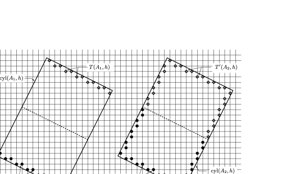
Figure 6: The sets $T(A,h)$, $B(A,h)$, $T^{\prime}(A,h)$ and $B^{\prime}(A,h)$ in $\operatorname{cyl}(A,h)$.

Let $T^{\prime}(A,h)$ [resp., $B^{\prime}(A,h)$] be the upper half part (resp., the lower half part) of the boundary of $\operatorname{cyl}(A,h)$ (see Figure 6); that is, if we denote by $z$ the center of $A$,

$$T^{\prime}(A,h)$$

$$\qquad=\left\{x\in\operatorname{cyl}(A,h)\left|\begin{array}[]{l}\overrightarrow{zx}\cdot\vec{v}>0\mbox{ and}\\ \exists y\notin\operatorname{cyl}(A,h),[x,y]\in\mathbb{E}^{d}_{n}\mbox{ and }[x,y]\cap\partial\operatorname{cyl}(A,h)\neq\varnothing\end{array}\right.\right\}$$

and

$$B^{\prime}(A,h)$$

$$\qquad=\left\{x\in\operatorname{cyl}(A,h)\left|\begin{array}[]{l}\overrightarrow{zx}\cdot\vec{v}<0\mbox{ and}\\ \exists y\notin\operatorname{cyl}(A,h),[x,y]\in\mathbb{E}^{d}_{n}\mbox{ and }[x,y]\cap\partial\operatorname{cyl}(A,h)\neq\varnothing\end{array}\right.\right\}.$$

For a given realization $(t(e),e\in\mathbb{E}_{n}^{d})$, we define the variable $\tau_{n}(A,h)=\break\tau_{n}(\operatorname{cyl}(A,h),\vec{v})$ by

$$\tau_{n}(A,h)=\tau_{n}\bigl{(}\operatorname{cyl}(A,h),\vec{v}\bigr{)}=\phi_{n}\bigl{(}T^{\prime}(A,h),B^{\prime}(A,h),\operatorname{cyl}(A,h)\bigr{)}.$$

The asymptotic behavior for large $n$ of the variable $\tau_{n}(A,h)$ properly rescaled is well known, thanks to the almost subadditivity of this variable. The following law of large numbers is proved in RossignolTheret08b :

Theorem 2.2 ((Rossignol and Théret))

We suppose that

$$\int_{[0,+\infty[}x\,d\Lambda(x)<\infty.$$

Then for each unit vector $\vec{v}$ there exists a constant $\nu(d,\Lambda,\vec{v})=\nu(\vec{v})$ (the dependence on $d$ and $\Lambda$ is implicit) such that for every non degenerate hyperrectangle $A$ orthogonal to $\vec{v}$ and for every strictly positive constant $h$, we have

$$\lim_{n\rightarrow\infty}\frac{\tau_{n}(A,h)}{n^{d-1}\mathcal{H}^{d-1}(A)}=\nu(\vec{v})\qquad\mbox{in }L^{1}.$$

Moreover, if the origin of the graph belongs to $A$, or if

$$\int_{[0,+\infty[}x^{1+{1}/{(d-1)}}\,d\Lambda(x)<\infty,$$

then

$$\lim_{n\rightarrow\infty}\frac{\tau_{n}(A,h)}{n^{d-1}\mathcal{H}^{d-1}(A)}=\nu(\vec{v})\qquad\mbox{a.s.}$$

We emphasize the fact that the limit $\nu(\vec{v})$ depends on the direction of $\vec{v}$, but neither on $h$ nor on the hyperrectangle $A$ itself. When the capacities of the edges are bounded [hypothesis (H2)], both $L^{1}$ and a.s. convergences hold in Theorem 2.2. This theorem gives the proper definition of the function $\nu$ that appeared in equation (5). The function $\nu$ is initially defined on $\SS^{d-1}$, but we consider its homogeneous extension to $\mathbb{R}^{d}$, that we still denote by $\nu$, defined by

$$\nu(\vec{0})=0\quad\mbox{and}\quad\forall\vec{w}\in\mathbb{R}^{d}\setminus\{\vec{0}\}\qquad\nu(\vec{w})=\|w\|_{2}\nu\biggl{(}\frac{\vec{w}}{\|\vec{w}\|_{2}}\biggr{)}.$$

We recall some geometric properties of the map $\nu$ that are valid whenever $\mathbb{E}(t(e))<\infty$. They have been stated in Section 4.4 of RossignolTheret08b . If there exists a unit vector $\vec{v}$ such that $\nu(\vec{v})=0$, then $\nu=0$ everywhere, and this happens if and only if $\Lambda(\{0\})\geq 1-p_{c}(d)$, where $p_{c}(d)$ denotes the critical parameter for bond percolation on $\mathbb{Z}^{d}$. This property has been proved by Zhang in Zhang . Moreover, the function $\nu:\mathbb{R}^{d}\rightarrow\mathbb{R}$ is convex. Since $\nu$ is finite, this implies that $\nu$ is continuous on $\mathbb{R}^{d}$. Moreover, $\nu$ is invariant under any transformation of $\mathbb{R}^{d}$ that preserves the graph $(\mathbb{Z}^{d},\mathbb{E}^{d})$, in particular $\nu(\vec{v})=\nu(-\vec{v})$ for all $\vec{v}\in\mathbb{R}^{d}$.

The asymptotic behavior of the maximal flow $\phi_{n}(\Gamma^{1}_{n},\Gamma^{2}_{n},\Omega_{n})$ was studied in the companion papers CerfTheret09supc , CerfTheret09geoc and CerfTheret09infc , and the following law of large numbers was proved:

Theorem 2.3 ((Cerf and Théret))

We suppose that the hypotheses (H1) and (H2) are fulfilled. Then there exists a finite constant $\phi_{\Omega}\geq 0$ defined in (33) and (37) such that

$$\lim_{n\rightarrow\infty}\frac{\phi_{n}}{n^{d-1}}=\phi_{\Omega}^{(1)}\qquad\mbox{a.s.}$$

Moreover, this equivalence holds:

$$\phi_{\Omega}^{(1)}>0\quad\iff\quad\Lambda\bigl{(}\{0\}\bigr{)}<1-p_{c}(d).$$

In fact the authors prove in CerfTheret09infc that the lower large deviations of $\phi_{n}/n^{d-1}$ below a constant $\phi_{\Omega}^{(1)}$ are of surface order, in CerfTheret09supc that the upper large deviations of $\phi_{n}/n^{d-1}$ above a constant $\phi_{\Omega}^{(2)}$ are of volume order and finally in CerfTheret09geoc that $\phi_{\Omega}^{(1)}=\phi_{\Omega}^{(2)}$. The definitions of $\phi_{\Omega}^{(1)}$ and $\phi_{\Omega}^{(2)}$ are the following:

$$\phi_{\Omega}^{(1)} = \inf\left\{\begin{array}[]{l}\displaystyle\int_{\Omega\cap\partial^{*}F}\nu\bigl{(}\vec{v}_{F}(x)\bigr{)}\,d\mathcal{H}^{d-1}(x)+\int_{\Gamma^{2}\cap\partial^{*}F}\nu\bigl{(}\vec{v}_{F}(x)\bigr{)}\,d\mathcal{H}^{d-1}(x)\\ \displaystyle\qquad{}+\int_{\Gamma^{1}\cap\partial^{*}(\Omega\setminus F)}\nu\bigl{(}\vec{v}_{\Omega}(x)\bigr{)}\,d\mathcal{H}^{d-1}(x)\end{array}\right.\left|\phantom{\begin{array}[]{l}\displaystyle\int_{\Omega\cap\partial^{*}F}\\ \displaystyle\qquad{}+\int_{\Gamma^{1}\cap\partial^{*}(\Omega\setminus F)}\end{array}}\right.$$ (33)

$$\hskip 106.0pt\left.\phantom{\begin{array}[]{l}\displaystyle\int_{\Omega\cap\partial^{*}F}\\ \displaystyle\qquad{}+\int_{\Gamma^{1}\cap\partial^{*}(\Omega\setminus F)}\end{array}}F\subset\Omega,\mathbh{1}_{F}\in\operatorname{BV}(\Omega)\right\},$$

$$\qquad\phi_{\Omega}^{(2)} = \inf\Biggl{\{}\int_{\Omega\cap\partial P}\nu\bigl{(}\vec{v}_{P}(x)\bigr{)}\,d\mathcal{H}^{d-1}(x)\Big{|}$$ (37)

$$\hskip 18.0pt\begin{array}[]{l}P\subset\,\mathbb{R}^{d},\overline{\Gamma}^{1}\subset\,\stackrel{{\scriptstyle\circ}}{{P}},\overline{\Gamma}^{2}\subset\,\stackrel{{\scriptstyle\circ}}{{\wideparen{\mathbb{R}^{d}\setminus P}}}\\ P\mbox{ is polyhedral},\partial P\mbox{ is transversal to }\Gamma\end{array}\Biggr{\}}.$$

The variational problems $\phi_{\Omega}^{(1)}$ and $\phi_{\Omega}^{(2)}$ are continuous min-cut problems very similar to the problem $\phi_{\Omega}^{(m)}$ defined by Nozawa. The variational problem $\phi_{\Omega}^{(1)}$ is in fact exactly the one we were looking for, that is, $\phi_{\Omega}^{a}=\phi_{\Omega}^{(1)}$, where $\phi_{\Omega}^{a}$ is the continuous min-cut problem appearing in Sections 1.2 and 1.3. Notice that a condition of the type “$\partial F$ separates $\Gamma^{1}$ from $\Gamma^{2}$ in $\Omega$” does not appear in $\phi_{\Omega}^{(1)}$, but the definition of the capacity of $F$ is adapted: the surface that is considered as “separating” is in fact the surface $(\partial F\cap\Omega)\cup(\partial F\cap\Gamma^{2})\cup(\partial(\Omega\setminus F)\cap\Gamma^{1})$ (see Figure 7). Thus we define for every $F\subset\Omega$ such that $\mathbh{1}_{F}\in\operatorname{BV}(\Omega)$,

$$\operatorname{capacity}(F) = \int_{\Omega\cap\partial^{*}F}\nu\bigl{(}\vec{v}_{F}(x)\bigr{)}\,d\mathcal{H}^{d-1}(x)+\int_{\Gamma^{2}\cap\partial^{*}F}\nu\bigl{(}\vec{v}_{F}(x)\bigr{)}\,d\mathcal{H}^{d-1}(x)$$

$${}+\int_{\Gamma^{1}\cap\partial^{*}(\Omega\setminus F)}\nu\bigl{(}\vec{v}_{\Omega}(x)\bigr{)}\,d\mathcal{H}^{d-1}(x),$$

and the variational problem $\phi^{(1)}$ can be rewritten as

$$\phi_{\Omega}^{a}=\phi_{\Omega}^{(1)}=\inf\bigl{\{}\operatorname{capacity}(F)|F\subset\Omega,\mathbh{1}_{F}\in\operatorname{BV}(\Omega)\bigr{\}}.$$

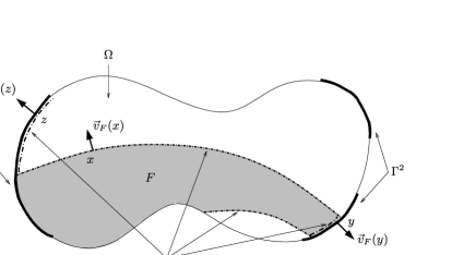
Figure 7: The set $(\partial F\cap\Omega)\cup(\partial F\cap\Gamma^{2})\cup(\partial(\Omega\setminus F)\cap\Gamma^{1})$.

Thus the set $\Sigma^{a}$ appearing in Theorem 1.2 is defined by

$$\Sigma^{a}=\bigl{\{}F\subset\Omega|\mathbh{1}_{F}\in\operatorname{BV}(\Omega),\operatorname{capacity}(F)=\phi_{\Omega}^{a}\bigr{\}}.$$

Let us prove that the min-cut problems $\phi_{\Omega}^{(1)}$, $\phi_{\Omega}^{(2)}$ and $\phi_{\Omega}^{(m)}$ are equivalent. We claim that

$$\phi_{\Omega}^{(1)}\leq\phi_{\Omega}^{(m)}\leq\phi_{\Omega}^{(2)}.$$ (38)

Since $\phi_{\Omega}^{(1)}=\phi_{\Omega}^{(2)}$ by CerfTheret09geoc , Theorem 11, we conclude that

$$\phi_{\Omega}^{(1)}=\phi_{\Omega}^{(2)}=\phi_{\Omega}^{(m)}.$$

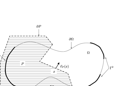
Figure 8: A polyhedral set $P$ as in the definition of $\phi_{\Omega}^{(2)}$.

Thus the three min-cut problems are equivalent. The arguments to justify inequality (38) are the following. On one hand, consider a set $P$ as in the definition (37) of $\phi_{\Omega}^{(2)}$ (see Figure 8), and define $S=P\cap\Omega$. Since $\overline{\Gamma}^{1}\subset\stackrel{{\scriptstyle\circ}}{{P}}$, then $\gamma(\mathbh{1}_{S})=1$ $\mathcal{H}^{d-1}$-a.e. on $\Gamma^{1}$ and since $\overline{\Gamma}^{2}\subset\,\stackrel{{\scriptstyle\circ}}{{\wideparen{\mathbb{R}^{d}\setminus P}}}$, then $\gamma(\mathbh{1}_{S})=0$ $\mathcal{H}^{d-1}$-a.e. on $\Gamma^{2}$, thus $S$ satisfies all the conditions required in the definition (22) of $\phi_{\Omega}^{(m)}$ and

$$\int_{\Omega\cap\partial^{*}S}\nu\bigl{(}\vec{v}_{S}(x)\bigr{)}\,d\mathcal{H}^{d-1}(x)=\int_{\Omega\cap\partial P}\nu\bigl{(}\vec{v}_{P}(x)\bigr{)}\,d\mathcal{H}^{d-1}(x).$$

Thus $\phi_{\Omega}^{(m)}\leq\phi_{\Omega}^{(2)}$. On the other hand consider a set $S$ as in the definition (22) of $\phi_{\Omega}^{(m)}$. Of course $S$ satisfies the conditions required in the definition (33) of $\phi_{\Omega}^{(1)}$. According to the last equality on page 809 in Nozawa , for every set $S\subset\Omega$ of finite perimeter in $\Omega$ we have

$$\gamma(\mathbh{1}_{S})=\mathbh{1}_{\Gamma\cap\partial^{*}S},\qquad\mathcal{H}^{d-1}\mbox{-a.e. on }\Gamma.$$ (39)

Thus $\gamma(\mathbh{1}_{S})=0$ $\mathcal{H}^{d-1}$-a.e. on $\Gamma^{2}$ implies that $\mathcal{H}^{d-1}(\Gamma^{2}\cap\partial^{*}S)=0$. By definition of the trace, $\gamma(\mathbh{1}_{\Omega\setminus S})=1-\gamma(\mathbh{1}_{S})$ everywhere on $\Gamma$, thus $\gamma(\mathbh{1}_{S})=1$ $\mathcal{H}^{d-1}$-a.e. on $\Gamma^{1}$ implies $\gamma(\mathbh{1}_{\Omega\setminus S})=0$ $\mathcal{H}^{d-1}$-a.e. on $\Gamma^{1}$. Since $\Omega\setminus S$ has also finite perimeter in $\Omega$, by equation (39) applied to $\Omega\setminus S$ we have $\gamma(\mathbh{1}_{\Omega\setminus S})=\mathbh{1}_{\Gamma\cap\partial^{*}(\Omega\setminus S)}$ $\mathcal{H}^{d-1}$-a.e. on $\Gamma$, thus $\mathcal{H}^{d-1}(\Gamma^{1}\cap\partial^{*}(\Omega\setminus S))=0$, and the integrals

$$\int_{\Gamma^{2}\cap\partial^{*}F}\nu\bigl{(}\vec{v}_{F}(x)\bigr{)}\,d\mathcal{H}^{d-1}(x)\quad\mbox{and}\quad\int_{\Gamma^{1}\cap\partial^{*}(\Omega\setminus F)}\nu\bigl{(}\vec{v}_{\Omega}(x)\bigr{)}\,d\mathcal{H}^{d-1}(x)$$

vanish. We conclude that $\phi_{\Omega}^{(1)}\leq\phi_{\Omega}^{(m)}$, and this finishes the proof of inequality (38).

Remark 9.

The simplicity of the previous argument should not hide that the real difficulty consists in proving that $\phi_{\Omega}^{(1)}=\phi_{\Omega}^{(2)}$. This is done in CerfTheret09geoc by a quite complicated process of polyhedral approximation.

3 Organization of the proof

In Section 4, we study a sequence of discrete maximal streams $(\vec{\mu}_{n}^{\max})_{n\geq 1}$. We prove that from each subsequence of $(\vec{\mu}_{n}^{\max})_{n\geq 1}$ we can extract a sub-subsequence which is weakly convergent. If we denote by $\vec{\mu}$ its limit, we prove that a.s. $\vec{\mu}=\vec{\sigma}\mathcal{L}^{d}$ with $\vec{\sigma}$ a continuous stream which is admissible for the max-flow problem $\phi_{\Omega}^{b}$. Moreover, we prove that along the converging subsequence,

$$\lim_{n\rightarrow\infty}\operatorname{flow}^{\mathrm{disc}}_{n}\bigl{(}\vec{\mu}_{n}^{\max}\bigr{)}=\operatorname{flow}^{\mathrm{cont}}(\vec{\sigma})\qquad\mbox{a.s.}$$ (40)

Section 5 is devoted to the study of a sequence of minimal cutsets $(\mathcal{E}_{n}^{\min})_{n\geq 1}$. We prove that from each subsequence of $(R(\mathcal{E}_{n}^{\min}))_{n\geq 1}$ we can extract a sub-subsequence which is convergent for the distance $\mathfrak{d}$. If we denote by $F$ its limit, we prove that $F\subset\Omega$ and $\mathbh{1}_{F}\in\operatorname{BV}(\Omega)$; that is, $F$ is admissible for the min-cut problem $\phi_{\Omega}^{a}$. Moreover, we prove that along the converging subsequence,

$$\liminf_{n\rightarrow\infty}\frac{V(\mathcal{E}_{n}^{\min})}{n^{d-1}}\geq\operatorname{capacity}(F)\qquad\mbox{a.s.}$$ (41)

In Section 6 we establish that

$$\operatorname{capacity}(F)\geq\operatorname{flow}^{\mathrm{cont}}(\vec{\sigma}).$$ (42)

Then combining equations (40), (41) and (42) we derive the results presented in Section 1.3.

The most original part of our work is the study of maximal streams presented in Section 4. The study of minimal cutsets relies largely on the techniques used in CerfTheret09infc to prove that the lower large deviations of $\phi_{n}$ are of surface order. To complete the proofs we also use the result of polyhedral approximation proved in CerfTheret09geoc . In the proof of the law of large numbers for $\phi_{n}$ we present here, we have replaced the study of the upper large deviations of $\phi_{n}$ performed in CerfTheret09supc by the study of the maximal streams, which is more natural, and we have adapted the arguments given in the study of the lower large deviations of $\phi_{n}$ in CerfTheret09infc to obtain informations on the behavior of minimal cutsets.

Throughout the paper, we assume that hypotheses (H1) and (H2) are satisfied.

4 Study of maximal streams

4.1 Existence

The existence of at least one maximal stream is not so obvious because of condition (2). We will assume throughout the paper that the capacities of the edges are bounded by a constant $M$. Under this hypothesis, the set $\mathcal{S}_{n}(\Gamma^{1}_{n},\Gamma^{2}_{n},\Omega_{n})$ is compact, and since the function $f_{n}\in\mathcal{S}_{n}(\Gamma^{1}_{n},\Gamma^{2}_{n},\Omega_{n})\mapsto\operatorname{flow}^{\mathrm{disc}}_{n}(\vec{\mu}_{n}(f_{n}))$ is continuous, a stream $\vec{\mu}_{n}=\vec{\mu}_{n}(f_{n})$ satisfying (1) exists. Suppose that $\vec{\mu}_{n}$ does not satisfy (2), and let $e=[a,b]$ with $a\in\Gamma^{1}_{n}$, $b\notin\Gamma^{1}_{n}$, and, for example, $\mathbf{e}=\langle a,b\rangle$ and $f_{n}(e)<0$. Since $f_{n}$ satisfies the node law and since there exists only a finite number of self avoiding paths (i.e., paths that visit each edge at most once) starting at $a$ in $\Omega_{n}$, then there exists a self avoiding path $r=(a,[a,b],b,\ldots,c)$ in $\Omega_{n}$ from $a$ to a point $c$ that belongs to $\Gamma^{1}_{n}$ or $\Gamma^{2}_{n}$ such that for all $e\in r$, if $r(e)=1$ (resp., $-1$) when $e$ is crossed by $r$ from the origin to the endpoint of $\mathbf{e}$ (resp., from the endpoint to the origin of $\mathbf{e}$), then $f_{n}(e)r(e)<0$. Since $r$ is finite,

$$m(f_{n},r)=\inf\bigl{\{}-f_{n}(e)r(e)|e\in r\bigr{\}}>0.$$

Consider the stream function $f_{n}^{\prime}$ defined by

$$f_{n}^{\prime}(e)=\cases{f_{n}(e),&\quad$\mbox{if }e\notin r,$\vspace*{2pt}\cr f_{n}(e)+r(e)m(f_{n},r),&\quad$\mbox{if }e\in r.$}$$

This is the stream function obtained by removing from $f_{n}$ a quantity of flow $m(f_{n},r)$ along $r$ from $c$ to $a$. The stream function $f_{n}^{\prime}$ is still admissible, since $|f_{n}^{\prime}(e)|\leq|f_{n}(e)|$ for all $e$. If $c$ belongs to $\Gamma^{2}_{n}$ (see Figure 9), then $\operatorname{flow}^{\mathrm{disc}}_{n}(\vec{\mu}_{n}(f_{n}^{\prime}))=\operatorname{flow}^{\mathrm{disc}}_{n}(\vec{\mu}_{n}(f_{n}))+m(f_{n},r)$, and this is not possible since $\vec{\mu}_{n}(f_{n})$ satisfies (1). Thus $c$ belongs to $\Gamma^{1}_{n}$ (see Figure 9) and $\operatorname{flow}^{\mathrm{disc}}_{n}(\vec{\mu}_{n}(f_{n}^{\prime}))=\operatorname{flow}^{\mathrm{disc}}_{n}(\vec{\mu}_{n}(f_{n}))$. Moreover, $f_{n}^{\prime}([a,b])=f_{n}([a,b])+m(f_{n},r)>f_{n}([a,b])$, and $m(f_{n}^{\prime},r)=0$. We can iterate this process finitely many times with every possible self avoiding path $r^{\prime}$ starting at $a$ until $m(f_{n},r^{\prime})=0$ for all $r^{\prime}$. Eventually, the stream function $f_{n}^{\prime\prime}$ we obtain satisfies $f_{n}^{\prime\prime}([a,b])=0$. We can do the same procedure with every edge $[a,b]$ with $a\in\Gamma^{1}_{n}$ and $b\notin\Gamma^{1}_{n}$ (there is a finite number of such edges), and the stream function $\widetilde{f}_{n}$ that we obtain at the end satisfies (2) and $\operatorname{flow}^{\mathrm{disc}}_{n}(\vec{\mu}_{n}(\widetilde{f}_{n}))=\operatorname{flow}^{\mathrm{disc}}_{n}(\vec{\mu}_{n}(f_{n}))$. This proves the existence of a maximal stream from $\Gamma^{1}_{n}$ to $\Gamma^{2}_{n}$ in $\Omega_{n}$ if we suppose that the capacities of the edges are bounded by a constant $M$.

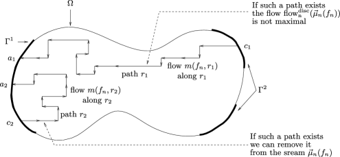
Figure 9: Flow that escapes from $\Omega_{n}$ through $\Gamma^{1}_{n}$.

From now on $(\vec{\mu}_{n})_{n\geq 1}$ denotes a sequence of admissible discrete streams and $(\vec{\mu}_{n}^{\max})_{n\geq 1}$ a sequence of admissible maximal discrete streams.

4.2 Compactness

We prove the following property:

Proposition 4.1

Almost surely, for $n$ large enough, the sequence$(\vec{\mu}_{n})_{n\geq 1}$ takes its values in a deterministic weakly compact set of measures.

Remark 10.

This property implies that any subsequence of $(\vec{\mu}_{n})_{n\geq 1}$ admits a sub-subsequence $(\vec{\mu}_{\varphi(n)})_{n\geq 1}$ that is weakly convergent, that is, such that there exists a random vector measure $\vec{\mu}\dvtx\mathcal{B}(\mathbb{R}^{d})\rightarrow\mathbb{R}^{d}$ satisfying

$$\forall f\in\mathcal{C}_{b}\bigl{(}\mathbb{R}^{d},\mathbb{R}\bigr{)}\qquad\lim_{n\rightarrow\infty}\int_{\mathbb{R}^{d}}f\,d\vec{\mu}_{\varphi(n)}=\int_{\mathbb{R}^{d}}f\,d\vec{\mu}.$$

The choice of the sub-subsequence $(\vec{\mu}_{\varphi(n)})_{n\geq 1}$ is random, that is, the function $\varphi$ may depend on the realization of the capacities.

Proof of Proposition 4.1 For the rest of this section, we consider a fixed realization of the capacities. Let $\vec{\mu}_{n}=(\mu_{n}^{1},\ldots,\mu_{n}^{d})$ be an admissible discrete stream on $(\mathbb{Z}^{d}_{n},\mathbb{E}^{d}_{n})$. For all $n\geq 1$, the support of $\vec{\mu}_{n}$ is included in the compact set $\overline{\mathcal{V}_{\infty}(\Omega,1)}$. Hence the admissible discrete streams are tight. Moreover, for $i=1,\ldots,d$, we have

$$\bigl{|}\mu^{i}_{n}\bigr{|}\bigl{(}\overline{\mathcal{V}_{\infty}(\Omega,1)}\bigr{)}\leq\frac{1}{n^{d}}\sum_{e\in\Pi_{n}}\bigl{|}f_{n}(e)\bigr{|}\leq\frac{M\operatorname{card}(\Pi_{n})}{n^{d}}.$$

Since

$$\operatorname{card}(\Pi_{n}) \leq 2d\operatorname{card}(\Omega_{n})\leq 2dn^{d}\mathcal{L}^{d}\biggl{(}\Omega+\frac{1}{2n}[-1,1]\biggr{)}$$

$$\leq 2dn^{d}\mathcal{L}^{d}\bigl{(}\mathcal{V}_{\infty}\bigl{(}\Omega,n^{-1}\bigr{)}\bigr{)}$$

$$\leq 2dn^{d}\mathcal{L}^{d}\bigl{(}\mathcal{V}_{\infty}(\Omega,1)\bigr{)},$$

we conclude that for all $i=1,\ldots,d$, for all $n\geq 1$,

$$\bigl{|}\mu^{i}_{n}\bigr{|}\bigl{(}\overline{\mathcal{V}_{\infty}(\Omega,1)}\bigr{)}\leq 2dM\mathcal{L}^{d}\bigl{(}\mathcal{V}_{\infty}(\Omega,1)\bigr{)}.$$

Thus the admissible discrete streams are uniformly bounded for the total variation distance. The conclusion follows from Prohorov’s theorem; see, for example, Theorem 8.6.2 in volume II of Bogachev .

Remark 11.

Since all the measures $\vec{\mu}_{n}$ have a support included in the same compact, the weak convergence $(\vec{\mu}_{n})_{n\geq 1}$ is characterized by the convergence of $\vec{\mu}_{n}(f)$ for all $f$ in any of the following classes of functions: the continuous bounded functions, the continuous functions with compact support or the continuous functions that goes to zero at infinity.

From now on, we consider a measure $\vec{\mu}$ which is the weak limit of a subsequence of $(\vec{\mu}_{n})_{n\geq 1}$, and we study its properties. Notice that $\vec{\mu}$ is a priori random, so some of its properties will be proved for all events, and others only a.s.

4.3 Absolute continuity with respect to Lebesgue measure

In this section, we prove that $\vec{\mu}$ is absolutely continuous with respect to $\mathcal{L}^{d}$, the Lebesgue measure on $\mathbb{R}^{d}$.

Proposition 4.2

If $\vec{\mu}$ is the weak limit of a subsequence of $(\vec{\mu}_{n})_{n\geq 1}$, where $\vec{\mu}_{n}$ is an admissible stream for all $n\geq 1$, then there exists a random vector field $\vec{\sigma}\dvtx\mathbb{R}^{d}\rightarrow\mathbb{R}^{d}$ such that $\vec{\mu}=\vec{\sigma}\mathcal{L}^{d}$, $\vec{\sigma}\in L^{\infty}(\mathbb{R}^{d}\rightarrow\mathbb{R}^{d},\mathcal{L}^{d})$ and $\vec{\sigma}=0$ $\mathcal{L}^{d}$-a.e. on $\Omega^{c}$.

For the rest of this section, we consider a fixed realization of the capacities. Let $\mu_{n}^{i}=\mu_{n}^{i,+}-\mu_{n}^{i,-}$ be the Hahn–Jordan decomposition of the signed measure $\mu_{n}^{i}$. Then $\mu_{n}^{i,+}$ and $\mu_{n}^{i,-}$ are positive measures on $(\mathbb{R}^{d},\mathcal{B}(\mathbb{R}^{d}))$, respectively, the positive and negative part of $\mu_{n}^{i}$. By the same arguments as in Proposition 4.1, we see that the sequences $(\mu_{n}^{i,+})_{n\geq 1}$ and $(\mu_{n}^{i,-})_{n\geq 1}$ take their value in a weakly compact set. Thus up to extraction we can suppose that $\vec{\mu}_{n}\rightharpoonup\vec{\mu}$, $\mu_{n}^{i,+}\rightharpoonup\mu^{i,+}$ and $\mu_{n}^{i,-}\rightharpoonup\mu^{i,-}$ for all $i=1,\ldots,d$, where $\mu^{i,+}$ and $\mu^{i,-}$ are positive measures. If we write $\vec{\mu}=(\mu^{1},\ldots,\mu^{d})$, we have $\mu^{i}=\mu^{i,+}-\mu^{i,-}$, but this may not be the Hahn–Jordan decomposition of $\mu^{i}$ since it may not be minimal. Let $B(x,r)$ be the ball centered at $x$ of radius $r>0$. We have

$$\mu_{n}^{i,+}\bigl{(}B(x,r)\bigr{)} \leq \bigl{|}\mu_{n}^{i}\bigr{|}\bigl{(}B(x,r)\bigr{)}\leq\frac{1}{n^{d}}\sum_{e\in\mathbb{E}^{d,i}_{n},c(e)\in B(x,r)}\bigl{|}f_{n}(e)\bigr{|}$$

$$\leq \frac{M\operatorname{card}(\{e\in\mathbb{E}^{d,i}_{n}|c(e)\in B(x,r)\})}{n^{d}},$$

and we remark as in Section 4.2 that

$$\operatorname{card}\bigl{(}\bigl{\{}e\in\mathbb{E}^{d,i}_{n}|c(e)\in B(x,r)\bigr{\}}\bigr{)} \leq \operatorname{card}\bigl{(}\mathbb{Z}^{d}_{n}\cap B\bigl{(}x,r+n^{-1}\bigr{)}\bigr{)}$$

$$\leq n^{d}\mathcal{L}^{d}\biggl{(}\mathbb{Z}^{d}_{n}\cap B\bigl{(}x,r+n^{-1}\bigr{)}+\frac{1}{2n}[-1,1]^{d}\biggr{)}$$

$$\leq n^{d}\mathcal{L}^{d}\bigl{(}B\bigl{(}x,r+2n^{-1}\bigr{)}\bigr{)},$$

whence

$$\mu_{n}^{i,+}\bigl{(}B(x,r)\bigr{)}\leq M\mathcal{L}^{d}\bigl{(}B\bigl{(}x,r+2n^{-1}\bigr{)}\bigr{)}.$$

With the help of Portmanteau’s theorem (see, e.g., Theorem 8.2.3 in Bogachev ) we obtain that

$$\mu^{i,+}\bigl{(}B(x,r)\bigr{)}\leq M\mathcal{L}^{d}\bigl{(}B(x,r)\bigr{)}.$$

Let next $A$ be a Borel subset of $\mathbb{R}^{d}$. Since the Lebesgue measure $\mathcal{L}^{d}$ is outer regular, for $\varepsilon>0$ there exists an open set $O$ such taht $A\subset O$ and $\mathcal{L}^{d}(O\setminus A)<\varepsilon$. By the Vitali covering theorem for Radon measures (see Theorem 2.8 in Mattila ), there exists a countable family $(B_{j},j\in J)$ of disjoint closed balls such that:

• $\forall j\in J\ B_{j}\subset O$;

• $\mu^{i,+}(O\setminus\bigcup_{j\in J}B_{j})=0$.

Thus

$$\mu^{i,+}(O)=\sum_{j\in J}\mu^{i,+}(B_{j})\leq M\sum_{j\in J}\mathcal{L}^{d}(B_{j})=M\mathcal{L}^{d}\biggl{(}\bigcup_{j\in J}B_{j}\biggr{)}\leq M\mathcal{L}^{d}(O),$$

whence

$$\mu^{i,+}(A)\leq\mu^{i,+}(O)\leq M\mathcal{L}^{d}(O)\leq M\bigl{(}\mathcal{L}^{d}(A)+\varepsilon\bigr{)}.$$

Sending $\varepsilon$ to $0$, we obtain that

$$\mu^{i,+}(A)\leq M\mathcal{L}^{d}(A).$$

We conclude that $\mu^{i,+}$ is absolutely continuous with respect to $\mathcal{L}^{d}$. The same holds for $\mu^{i,-}$, for all $i=1,\ldots,d$, thus $\vec{\mu}$ is absolutely continuous with respect to $\mathcal{L}^{d}$; that is, there exists $\vec{\sigma}\in L^{1}(\mathbb{R}^{d}\rightarrow\mathbb{R}^{d},\mathcal{L}^{d})$ such that $\vec{\mu}=\vec{\sigma}\mathcal{L}^{d}$. We use the notation $\vec{\sigma}=(\sigma^{1},\ldots,\sigma^{d})$. Moreover we have proved that for all $i=1,\ldots,d$,

$$\forall A\in\mathcal{B}\bigl{(}\mathbb{R}^{d}\bigr{)}\qquad\int_{A}\bigl{|}\sigma^{i}\bigr{|}\,d\mathcal{L}^{d}\leq\mu^{i,+}(A)+\mu^{i,-}(A)\leq 2M\mathcal{L}^{d}(A),$$

which implies that $|\sigma^{i}|\leq 2M$ $\mathcal{L}^{d}$-a.e. and thus that $\vec{\sigma}$ belongs to $L^{\infty}(\mathbb{R}^{d}\rightarrow\mathbb{R}^{d},\mathcal{L}^{d})$. Finally, we notice that for $n\geq 1$, the support of $\vec{\mu}_{n}$ is included in $\mathcal{V}_{\infty}(\Omega,1/n)$, thus the support of $\vec{\mu}$ is included in $\bigcap_{n\geq 1}\mathcal{V}_{\infty}(\Omega,1/n)=\overline{\Omega}$. This implies that $\vec{\sigma}=0$ $\mathcal{L}^{d}$-a.e. on $\mathbb{R}^{d}\setminus\overline{\Omega}$, thus on $\Omega^{c}$ since $\mathcal{L}^{d}(\partial\Omega)=0$.

4.4 Divergence and boundary conditions

We study the divergence of $\vec{\sigma}$. We recall that divergence must be understood in the distributional sense. By definition, for every function $h\in\mathcal{C}_{c}^{\infty}(\mathbb{R}^{d},\mathbb{R})$, we have

$$\int_{\mathbb{R}^{d}}h\operatorname{div}\vec{\sigma}\,d\mathcal{L}^{d}=-\int_{\mathbb{R}^{d}}\vec{\sigma}\cdot\vec{\nabla}h\,d\mathcal{L}^{d}.$$ (44)

We first prove the following result:

Proposition 4.3

If $\vec{\mu}=\vec{\sigma}\mathcal{L}^{d}$ is the weak limit of a subsequence $(\vec{\mu}_{\varphi(n)})_{n\geq 1}$ of $(\vec{\mu}_{n})_{n\geq 1}$, then for every function $h\in\mathcal{C}_{c}^{\infty}(\mathbb{R}^{d},\mathbb{R})$ we have

$$\int_{\mathbb{R}^{d}}h\operatorname{div}\vec{\sigma}\,d\mathcal{L}^{d} = -\int_{\mathbb{R}^{d}}\vec{\sigma}\cdot\vec{\nabla}h\,d\mathcal{L}^{d}$$

$$= \lim_{n\rightarrow\infty}\frac{1}{\varphi(n)^{d-1}}\sum_{x\in\Gamma^{1}_{\varphi(n)}\cup\Gamma^{2}_{\varphi(n)}}h(x)\widehat{f}_{\varphi(n)}(x),$$

where for all $x\in(\Gamma^{1}_{n}\cup\Gamma^{2}_{n})$, $\widehat{f}_{n}(x)$ is the amount of water that appears at $x$ according to the stream $f_{n}$:

$$\widehat{f}_{n}(x)=\sum_{e=\langle\cdot,x\rangle}f_{n}(e)-\sum_{e=\langle x,\cdot\rangle}f_{n}(e).$$

The idea of the proof is the following: we interpret $\operatorname{div}\vec{\sigma}$ as the limit of a discrete divergence, which we can control thanks to the node law satisfied by the stream function $f_{n}$. We consider again a fixed realization of the capacities. We consider a subsequence of $(\vec{\mu}_{n})_{n\geq 1}$ converging toward $\vec{\mu}$, but we still denote this subsequence by $(\vec{\mu}_{n})_{n\geq 1}$ to simplify the notation. Since $\vec{\nabla}h\in\mathcal{C}_{b}(\mathbb{R}^{d},\mathbb{R}^{d})$, we see that

$$\quad\int_{\mathbb{R}^{d}}\vec{\sigma}\cdot\vec{\nabla}h\,d\mathcal{L}^{d}=\lim_{n\rightarrow\infty}\int_{\mathbb{R}^{d}}\vec{\nabla}h\cdot d\vec{\mu}_{n}=\lim_{n\rightarrow\infty}\frac{1}{n^{d}}\sum_{e\in\mathbb{E}_{n}^{d}}f_{n}(e)\vec{e}\cdot\vec{\nabla}h\bigl{(}c(e)\bigr{)}.$$ (46)

We study the sum appearing in the previous equality. Let $i\in\{1,\ldots,d\}$. By Taylor’s theorem, we know that for all $x=(x_{1},\ldots,x_{d}),y=(y_{1},\ldots,y_{d})\in\mathbb{R}^{d}$ such that $x_{j}=y_{j}$ for all $j\neq i$ we have

$$h(x)-h(y)=\partial_{i}h(y)(x_{i}-y_{i})+g(x,y),$$

and since $h$ is in $\mathcal{C}^{2}_{c}(\mathbb{R}^{d},\mathbb{R})$ we know that $|g(x,y)|\leq K(x_{i}-y_{i})^{2}$, where $K=K(h)=\|h\|_{W^{2,\infty}}/2$. For $e\in\mathbb{E}^{d,i}_{n}$, let us denote by $l_{i}(e)$ [resp., $r_{i}(e)$] the endpoint at the origin (resp., the end) of $\mathbf{e}$ according to the orientation

Figure 10: Correspondence between edges and vertices.

chosen on $\mathbb{E}^{d,i}_{n}$; see Figure 10. Conversely, for $x\in\mathbb{Z}^{d}_{n}$, we denote by $L^{i}(x)$ [resp., $R^{i}(x)$] the edge of $\mathbb{E}^{d,i}_{n}$ which ends at $x$ (resp., starts at $x$).We obtain

$$\sum_{e\in\mathbb{E}^{d}_{n}}f_{n}(e)\vec{e}\cdot\vec{\nabla}h\bigl{(}c(e)\bigr{)}$$

$$\qquad=\sum_{i=1}^{d}\sum_{e\in\mathbb{E}^{d,i}_{n}}f_{n}(e)\partial_{i}h\bigl{(}c(e)\bigr{)}$$

$$\qquad=\sum_{i=1}^{d}\sum_{e\in\mathbb{E}^{d,i}_{n}}f_{n}(e)n\bigl{(}\bigl{[}h\bigl{(}r_{i}(e)\bigr{)}-h\bigl{(}l_{i}(e)\bigr{)}\bigr{]}-\bigl{[}g\bigl{(}r_{i}(e),c(e)\bigr{)}-g\bigl{(}c(e),l_{i}(e)\bigr{)}\bigr{]}\bigr{)}$$

$$\qquad=n\sum_{x\in\mathbb{Z}^{d}_{n}}h(x)\sum_{i=1}^{d}\bigl{[}f_{n}\bigl{(}L_{i}(x)\bigr{)}-f_{n}\bigl{(}R_{i}(x)\bigr{)}\bigr{]}+\alpha_{n}(h,f,\Omega),$$

where by inequality (4.2) we have

$$\bigl{|}\alpha_{n}(h,f,\Omega)\bigr{|}\leq n\frac{2K}{(2n)^{2}}M\operatorname{card}(\Pi_{n})\leq dKM\mathcal{L}^{d}\bigl{(}\mathcal{V}_{\infty}(\Omega,1)\bigr{)}n^{d-1}.$$ (47)

Since the stream satisfies the node law, we have for all $x\notin(\Gamma^{1}_{n}\cup\Gamma^{2}_{n})$ that

$$\sum_{i=1}^{d}\bigl{[}f_{n}\bigl{(}L_{i}(x)\bigr{)}-f_{n}\bigl{(}R_{i}(x)\bigr{)}\bigr{]}=0.$$

For all $x\in(\Gamma^{1}_{n}\cup\Gamma^{2}_{n})$, let us denote by $\widehat{f}_{n}(x)$ the amount of water that appears at $x$ according to the stream $f_{n}$, that is,

$$\widehat{f}_{n}(x)=\sum_{i=1}^{d}\bigl{[}f_{n}\bigl{(}R_{i}(x)\bigr{)}-f_{n}\bigl{(}L_{i}(x)\bigr{)}\bigr{]}=\sum_{e=\langle\cdot,x\rangle}f_{n}(e)-\sum_{e=\langle x,\cdot\rangle}f_{n}(e).$$ (48)

Then we have proved that

$$\int_{\mathbb{R}^{d}}\vec{\nabla}h\cdot d\vec{\mu}_{n}=-\frac{1}{n^{d-1}}\sum_{x\in\Gamma^{1}_{n}\cup\Gamma^{2}_{n}}h(x)\widehat{f}_{n}(x)+\frac{\alpha_{n}(h,f,\Omega)}{n^{d}}.$$

According to equations (46) and (47), this implies equation (4.3), and thus Proposition 4.3 is proved.

We now deduce from Proposition 4.3 that $\operatorname{div}\vec{\sigma}$ and $\vec{\sigma}\cdot\vec{v}_{\Omega}$ satisfy the conditions required in Nozawa . Remember that divergence is understood in the distributional sense. The meaning of $\vec{\sigma}\cdot\vec{v}_{\Omega}$ is the one given by Nozawa in Nozawa that we have recalled in Section 2.2.

Corollary 2

If $\vec{\mu}=\vec{\sigma}\mathcal{L}^{d}$ is the limit of a subsequence of $(\vec{\mu}_{n})_{n\geq 1}$, then it satisfies $\operatorname{div}\vec{\sigma}=0$ $\mathcal{L}^{d}$-a.e. on $\Omega$ and $\vec{\sigma}\cdot\vec{v}_{\Omega}=0$ $\mathcal{H}^{d-1}$-a.e. on $\Gamma\setminus(\Gamma^{1}\cup\Gamma^{2})$. Moreover, if for all $n\geq 1$, $\widehat{f}_{n}(x):=\sum_{e=\langle\cdot,x\rangle}f_{n}(e)-\sum_{e=\langle x,\cdot\rangle}f_{n}(e)\geq 0$ for all $x\in\Gamma^{1}_{n}$ then $\vec{\sigma}\cdot\vec{v}_{\Omega}\leq 0$ $\mathcal{H}^{d-1}$-a.e. on $\Gamma^{1}$.

Remark 12.

By definition, the last condition is satisfied by a sequence of maximal flows $(\vec{\mu}_{n}^{\max})_{n\geq 1}$.

Proof of Corollary 2 We consider a fixed realization of the capacities. We prove first that $\operatorname{div}\vec{\sigma}=0$ on $\Omega$ in terms of distributions. Indeed, for every function $h\in\mathcal{C}_{c}^{\infty}(\Omega,\mathbb{R})$, $h$ is null on $\Gamma^{1}_{n}\cup\Gamma^{2}_{n}$, for all $n$. Thus by Proposition 4.3,

$$\int_{\mathbb{R}^{d}}h\operatorname{div}\vec{\sigma}\,d\mathcal{L}^{d}=-\int_{\mathbb{R}^{d}}\vec{\sigma}\cdot\vec{\nabla}h\,d\mathcal{L}^{d}=0.$$

As explained in Remark 6, we rewrite this equality as $\operatorname{div}\vec{\sigma}=0$ $\mathcal{L}^{d}$-a.e. on $\Omega$. We now study the boundary conditions satisfied by $\vec{\sigma}$. As explained in Section 2.2, $\vec{\sigma}\cdot\vec{v}_{\Omega}$ is an element of $L^{\infty}(\Gamma,\mathcal{H}^{d-1})$ characterized by

$$\forall u\in W^{1,1}(\Omega)\qquad\int_{\Gamma}(\vec{\sigma}\cdot\vec{v}_{\Omega})\gamma(u)\,d\mathcal{H}^{d-1}=\int_{\Omega}\vec{\sigma}\cdot\vec{\nabla}u\,d\mathcal{L}^{d}.$$ (49)

In fact $\vec{\sigma}\cdot\vec{v}_{\Omega}$ is characterized by

$$\forall u\in\mathcal{C}_{c}^{\infty}\bigl{(}\mathbb{R}^{d},\mathbb{R}\bigr{)}\qquad\int_{\Gamma}(\vec{\sigma}\cdot\vec{v}_{\Omega})u\,d\mathcal{H}^{d-1}=\int_{\mathbb{R}^{d}}\vec{\sigma}\cdot\vec{\nabla}u\,d\mathcal{L}^{d}.$$ (50)

Let us prove that the conditions (49) and (50) are equivalent. We recall that $W^{1,1}(\Omega)$ is the set of functions $u\dvtx\Omega\rightarrow\mathbb{R}$ satisfying $u\in L^{1}(\Omega)$, and for all $i\in\{1,\ldots,d\}$, there exists $g_{i}\in L^{1}(\Omega)$ such that

$$\forall h\in\mathcal{C}^{\infty}_{c}(\Omega,\mathbb{R})\qquad\int_{\Omega}u\partial_{i}h\,d\mathcal{L}^{d}=-\int_{\Omega}g_{i}h\,d\mathcal{L}^{d}.$$

By definition $\|\partial_{i}u\|_{L^{1}(\Omega)}=\|g_{i}\|_{L^{1}(\Omega)}$. The norm on the Sobolev space $W^{1,1}(\Omega)$ is given by

$$\forall u\in W^{1,1}(\Omega)\qquad\|u\|_{W^{1,1}(\Omega)}=\|u\|_{L^{1}(\Omega)}+\sum_{i=1}^{d}\|\partial_{i}u\|_{L^{1}(\Omega)}.$$

The set of functions $\{f|_{\Omega},f\in\mathcal{C}_{c}^{\infty}(\mathbb{R}^{d},\mathbb{R})\}$ is dense into $W^{1,1}(\Omega)$ with respect to the norm $\|\cdot\|_{W^{1,1}(\Omega)}$ (see, e.g., Nozawa , page 809). Let $u\in W^{1,1}(\Omega)$ and $(u_{n})_{n\geq 1}$ be a sequence of functions in $\mathcal{C}_{c}^{\infty}(\mathbb{R}^{d},\mathbb{R})$ such that $\tilde{u}_{n}=u_{n}|_{\Omega}$ converges toward $u$ in $W^{1,1}(\Omega)$. Then $u$ and $\tilde{u}_{n}$ belong to $\operatorname{BV}(\Omega)$ for all $n\geq 1$, and $\tilde{u}_{n}$ converges toward $u$ in $\operatorname{BV}(\Omega)$ in the sense given by Nozawa in Nozawa , page 808; that is, $\tilde{u}_{n}$ converges toward $u$ in $L^{1}(\Omega)$ and $|\vec{\nabla}\tilde{u}_{n}|(\Omega)$ converges toward $|\vec{\nabla}u|(\Omega)$. Then by Nozawa , Theorem 2.1 (that comes from GI ), we know that $\gamma(\tilde{u}_{n})=u_{n}|_{\Gamma}$ converges toward $\gamma(u)$ in $L^{1}(\Gamma)$. Since $\vec{\sigma}\cdot\vec{v}_{\Omega}$ is in $L^{\infty}(\Gamma)$, this implies that

$$\lim_{n\rightarrow\infty}\int_{\Gamma}(\vec{\sigma}\cdot\vec{v}_{\Omega})u_{n}\,d\mathcal{H}^{d-1}=\int_{\Gamma}(\vec{\sigma}\cdot\vec{v}_{\Omega})\gamma(u)\,d\mathcal{H}^{d-1}.$$ (51)

Moreover, since $\vec{\sigma}\in L^{\infty}(\Omega,\mathbb{R}^{d})$, the convergence of $\tilde{u}_{n}$ toward $u$ in $W^{1,1}(\Omega)$ implies

$$\lim_{n\rightarrow\infty}\int_{\Omega}\vec{\sigma}\cdot\vec{\nabla}\tilde{u}_{n}\,d\mathcal{L}^{d}=\int_{\Omega}\vec{\sigma}\cdot\vec{\nabla}u\,d\mathcal{L}^{d}.$$ (52)

Finally, $\vec{\sigma}=0$ $\mathcal{L}^{d}$-a.e. on $\Omega^{c}$ implies that

$$\int_{\Omega}\vec{\sigma}\cdot\vec{\nabla}\tilde{u}_{n}\,d\mathcal{L}^{d}=\int_{\Omega}\vec{\sigma}\cdot\vec{\nabla}u_{n}\,d\mathcal{L}^{d}=\int_{\mathbb{R}^{d}}\vec{\sigma}\cdot\vec{\nabla}u_{n}\,d\mathcal{L}^{d}.$$ (53)

Combining equations (51), (52) and (53), we conclude that properties (49) and (50) are equivalent. According to (4.3), we obtain that for all $u\in\mathcal{C}_{c}^{\infty}(\mathbb{R}^{d},\mathbb{R})$,

$$\int_{\Gamma}(\vec{\sigma}\cdot\vec{v}_{\Omega})u\,d\mathcal{H}^{d-1}=\lim_{n\rightarrow\infty}-\frac{1}{n^{d-1}}\sum_{x\in\Gamma_{n}^{1}\cup\Gamma^{2}_{n}}u(x)\widehat{f}_{n}(x).$$

On one hand, let $u$ be a function of $\in\mathcal{C}_{c}^{\infty}((\Gamma^{1}\cup\Gamma^{2})^{c},\mathbb{R})$, that is, $u$ is defined on $\mathbb{R}^{d}$, takes values in $\mathbb{R}$, is of class $\mathcal{C}^{\infty}$ and its domain is contained in a compact subset of $(\Gamma^{1}\cup\Gamma^{2})^{c}$. Then for $n$ large enough, $u$ is null on $\Gamma^{1}_{n}\cup\Gamma^{2}_{n}$, thus

$$\int_{\Gamma}(\vec{\sigma}\cdot\vec{v}_{\Omega})u\,d\mathcal{H}^{d-1}=0,$$

and we conclude that $\vec{\sigma}\cdot\vec{v}_{\Omega}=0$, $\mathcal{H}^{d-1}$-a.e. on $\Gamma\setminus(\Gamma^{1}\cup\Gamma^{2})$. On the other hand, if $u\in\mathcal{C}_{c}^{\infty}((\Gamma\setminus\Gamma^{1})^{c},\mathbb{R})$, then for $n$ large enough,

$$\int_{\Gamma}(\vec{\sigma}\cdot\vec{v}_{\Omega})u\,d\mathcal{H}^{d-1}=\lim_{n\rightarrow\infty}-\frac{1}{n^{d-1}}\sum_{x\in\Gamma_{n}^{1}}u(x)\widehat{f}_{n}(x),$$

and if for all $n\geq 1$ we have $\widehat{f}_{n}(x)\geq 0$ for all $x\in\Gamma^{1}_{n}$, then we conclude that $\vec{\sigma}\cdot\vec{v}_{\Omega}\leq 0$ $\mathcal{H}^{d-1}$-a.e. on $\Gamma^{1}$.

Remark 13.

Notice that combining equations (44) and (50), we obtain that

$$\forall h\in C_{c}^{\infty}\bigl{(}\mathbb{R}^{d},\mathbb{R}\bigr{)}\qquad\int_{\mathbb{R}^{d}}h\operatorname{div}\vec{\sigma}\,d\mathcal{L}^{d}=-\int_{\Gamma}h(\vec{\sigma}\cdot\vec{v}_{\Omega})\,d\mathcal{H}^{d-1}.$$ (54)

This implies that $\operatorname{div}\vec{\sigma}$ is a distribution of order $0$ on $\mathbb{R}^{d}$,

$$\forall K\mbox{ compact of }\mathbb{R}^{d},\exists C_{K},\forall h\in\mathcal{C}^{\infty}_{c}(K,\mathbb{R})\qquad\biggl{|}\int_{\mathbb{R}^{d}}h\operatorname{div}\vec{\sigma}\,d\mathcal{L}^{d}\biggr{|}\leq C_{K}\|h\|_{\infty},$$

since we can choose $C_{K}=C=\|\vec{\sigma}\cdot\vec{v}_{\Omega}\|_{\infty}\mathcal{H}^{d-1}(\Gamma)$ for any compact $K$. Thus by the Riesz representation theorem (see Theorem 6.19 in Rudinrc ) we know that it is a Radon measure that we denote by $\operatorname{div}\vec{\sigma}\mathcal{L}^{d}$, and this measure is completely characterized by equation (54), that is,

$$\operatorname{div}\vec{\sigma}\mathcal{L}^{d}=-(\vec{\sigma}\cdot\vec{v}_{\Omega})\mathcal{H}^{d-1}|_{\Gamma}.$$ (55)

4.5 Capacity constraint

In this section, we prove the following proposition:

Proposition 4.4

If $\vec{\mu}=\vec{\sigma}\mathcal{L}^{d}$ is the limit of a subsequence of $(\vec{\mu}_{n})_{n\geq 1}$, then almost surely we have

$$\mathcal{L}^{d}\mbox{-a.e. on }\mathbb{R}^{d},\forall\vec{v}\in\SS^{d-1}\qquad\vec{\sigma}\cdot\vec{v}\leq\nu(\vec{v}).$$ (56)

We explain first the idea of the proof. The convergence $\vec{\mu}_{n}\rightharpoonup\vec{\sigma}\mathcal{L}^{d}$ implies that

$$\int_{D}\vec{\sigma}\cdot\vec{v}\,d\mathcal{L}^{d}=\lim_{n\rightarrow\infty}\int_{D}\,d\vec{\mu}_{n}\cdot\vec{v}$$

for every Borel set $D$ such that $\mathcal{L}^{d}(\partial D)=0$. On one hand, using Lebesgue differentiation theorem, we know that for $\mathcal{L}^{d}$-a.e. $x$,

$$\frac{1}{\mathcal{L}^{d}(D(x,\varepsilon))}\int_{D(x,\varepsilon)}\vec{\sigma}\cdot\vec{v}\,d\mathcal{L}^{d}$$

converges toward $\vec{\sigma}(x)\cdot\vec{v}$ when $\varepsilon$ goes to zero, where $D(x,\varepsilon)$ is a “nice” sequence of neighborhoods of $x$ of diameter $\varepsilon$. To conclude that $\vec{\sigma}\cdot\vec{v}$ is bounded by $\nu(\vec{v})$, it remains to compare $\int_{D}\,d\vec{\mu}_{n}\cdot\vec{v}$ with $\nu(\vec{v})$. Proposition 4.5 states that when $D$ is a cylinder of height $h$ in the direction $\vec{v}$, $\int_{D}\,d\vec{\mu}_{n}\cdot\vec{v}$ is close to $h\Psi(\vec{\mu}_{n},D,\vec{v})/n^{d-1}$, where $\Psi(\vec{\mu}_{n},D,\vec{v})$ is the amount of fluid that crosses $D$ from the lower half part to the upper half part of its boundary in the direction $\vec{v}$ according to the stream $\vec{\mu}_{n}$. Since $\tau_{n}(D,\vec{v})$ is the maximal value of such a flow, $\Psi(\vec{\mu}_{n},D,\vec{v})\leq\tau_{n}(D,\vec{v})$, and we can conclude the proof by using the convergence of the rescaled flow $\tau_{n}(D,\vec{v})$ toward $\nu(\vec{v})$. The key argument—and the less intuitive—is Proposition 4.5. In fact, if $\vec{l}$ is a $\mathcal{C}^{1}$ vector field on $D$ with null divergence and such that $\vec{l}\cdot\vec{v}_{D}=0$ $\mathcal{H}^{d-1}$-a.e. on the vertical faces of $D$ (the ones who are not normal to $\vec{v}$), if we denote by $B$ the basis of $D$, then by Fubini theorem we have

$$\int_{D}\vec{l}\cdot\vec{v}\,d\mathcal{L}^{d}=\int_{0}^{h}\biggl{(}\int_{B+u\vec{v}}\vec{l}\cdot\vec{v}\,d\mathcal{H}^{d-1}\biggr{)}\,du$$

and we have for all u

$$\int_{B+u\vec{v}}\vec{l}\cdot\vec{v}\,d\mathcal{H}^{d-1}=\int_{B}\vec{l}\cdot\vec{v}\,d\mathcal{H}^{d-1}$$

since by the Gauss–Green theorem we get

$$\int_{\partial D}\vec{l}\cdot\vec{v}_{D}\,d\mathcal{H}^{d-1}=\int_{D}\operatorname{div}\vec{l}\,d\mathcal{L}^{d}=0.$$

We obtain that

$$\int_{D}\vec{l}\cdot\vec{v}\,d\mathcal{L}^{d}=h\int_{B}\vec{l}\cdot\vec{v}\,d\mathcal{H}^{d-1}$$

and $\int_{B}\vec{l}\cdot\vec{v}\,d\mathcal{H}^{d-1}$ is indeed the flow that goes from the bottom to the top of $D$ according to $\vec{l}$. In the proof of Proposition 4.5, we adapt this argument to a discrete stream $\vec{\mu}_{n}$, and we consider a cylinder flat enough (i.e., $h$ small enough) to control the amount of fluid that enters in $D$ or escapes from $D$ through its vertical faces.

Step 1: From $\vec{\sigma}(x)\cdot\vec{v}$ to $\int_{cyl(x_{p}+p^{-1}A,p^{-1}h)}\vec{\sigma}\cdot\vec{v}\,d\mathcal{L}^{d}$. Since the functions $\vec{v}\in\SS^{d-1}\mapsto\vec{\sigma}(x)\cdot\vec{v}$ (for a fixed realization and a fixed $x$) and $\vec{v}\in\SS^{d-1}\mapsto\nu(\vec{v})$ are continuous, property (56) is equivalent to

$$\mathcal{L}^{d}\mbox{-a.e. on }\mathbb{R}^{d},\forall\vec{v}\in\widehat{\SS}^{d-1}\qquad\vec{\sigma}\cdot\vec{v}\leq\nu(\vec{v}),$$ (57)

where $\widehat{\SS}^{d-1}$ denotes the set of all the unit vectors of $\mathbb{R}^{d}$ that define a rational direction. Theorem 2.2 states that for every cylinder $\operatorname{cyl}(A,h)$ with $A$ a non degenerate hyperrectangle normal to $\vec{v}$ and $h>0$, we have

$$\lim_{n\rightarrow\infty}\frac{\tau_{n}(\operatorname{cyl}(A,h),\vec{v})}{n^{d-1}\mathcal{H}^{d-1}(A)}=\nu(\vec{v})\qquad\mbox{a.s.}$$ (58)

Thus these convergences hold a.s. simultaneously for all cylinders $\operatorname{cyl}(A,h)$ whose vertices have rational coordinates. For the rest of this section, we consider a fixed realization of the capacities on which these convergences happen.

According to Definition 7.9 in Rudinrc , we say that a sequence $(V_{p})_{p\geq 1}$ of Borel sets in $\mathbb{R}^{d}$ shrinks to a point $x\in\mathbb{R}^{d}$ nicely if there exists a number $\alpha>0$ and a sequence of positive real numbers $(r_{p})_{p\geq 1}$ satisfying $\lim_{p\rightarrow\infty}r_{p}=0$, and for all $p\geq 1$,

$$V_{p}\subset B(x,r_{p})\quad\mbox{and}\quad\mathcal{L}^{d}(V_{p})\geq\alpha\mathcal{L}^{d}\bigl{(}B(x,r_{p})\bigr{)}.$$

We need the Lebesgue differentiation theorem on $\mathbb{R}^{d}$ (see Theorem 7.10 in Rudinrc ):

Theorem 4.1

Let $g$ be a Borel function in $L^{1}(\mathbb{R}^{d},\mathcal{L}^{d})$. To each $x\in\mathbb{R}^{d}$, associate a sequence $(V_{p}(x))_{p\geq 1}$ of Borel sets in $\mathbb{R}^{d}$ that shrinks to $x$ nicely. Then for $\mathcal{L}^{d}$-a.e. $x\in\mathbb{R}^{d}$,

$$\lim_{p\rightarrow\infty}\frac{1}{\mathcal{L}^{d}(V_{p}(x))}\int_{V_{p}(x)}g\,d\mathcal{L}^{d}=g(x).$$

To each point $x\in\mathbb{R}^{d}$, we associate a deterministic sequence $(x_{p}(x))_{p\geq 1}$ of points of $\mathbb{R}^{d}$ that have rational coordinates and satisfying $\|x_{p}(x)-x\|\leq 1/p$. Then for every nondegenerate cylinder $D$ of center $0$, the sequence of Borel sets $(x_{p}(x)+p^{-1}D)_{p\geq 1}$ shrinks to $x$ nicely. We apply Theorem 4.1 to the function $\vec{\sigma}$ (coordinate by coordinate) to obtain that for $\mathcal{L}^{d}$-a.e. $x$, for every cylinder $D=\operatorname{cyl}(A,h)$ of center $0$ and whose vertices have rational coordinates (we say that $D$ is a rational cylinder), we have

$$\lim_{p\rightarrow\infty}\frac{1}{p^{-d}\mathcal{L}^{d}(D)}\int_{x_{p}(x)+p^{-1}D}\vec{\sigma}\,d\mathcal{L}^{d}=\vec{\sigma}(x).$$

From now on, we consider a fixed $x$ [thus a fixed sequence $(x_{p}(x))_{p\geq 1}$ that we denote by $(x_{p})_{p\geq 1}$] such that the previous convergence holds for every rational cylinder $D$.

Let $\vec{v}$ be a vector in $\widehat{\SS}^{d-1}$ and $\eta$ a positive real number. There exists a positive real number $\lambda$ such that $\lambda\vec{v}$ has integer coordinates. If $(\vec{\mathbf{f}}_{1},\ldots,\vec{\mathbf{f}}_{d})$ is the canonical basis on $\mathbb{R}^{d}$, suppose for instance $\lambda^{\prime}\vec{v}\cdot\vec{\mathbf{f}}_{1}\neq 0$, then $(\lambda^{\prime}\vec{v},\vec{\mathbf{f}}_{2},\ldots,\vec{\mathbf{f}}_{d})$ is a basis of $\mathbb{R}^{d}$. Adapting slightly the Gram–Schmidt process, we can obtain an orthogonal basis $(\vec{v},\vec{u}_{2},\ldots,\vec{u}_{d})$ of $\mathbb{R}^{d}$ such that all the vectors $\vec{u}_{i}$, $i=2,\ldots,d$ have integer coordinates. Thus there exists a non degenerate hyperrectangle $A$ of center $0$, normal to $\vec{v}$ and whose vertices have rational coordinates. Then for every positive rational number $h$ [thus $\operatorname{cyl}(A,h)$ is a rational cylinder], there exists $p_{0}(x,A,h,\eta)<\infty$ such that for all $p\geq p_{0}$ we get

$$\biggl{|}\frac{1}{\mathcal{L}^{d}(\operatorname{cyl}(x_{p}+p^{-1}A,p^{-1}h))}\int_{\operatorname{cyl}(x_{p}+p^{-1}A,p^{-1}h)}\vec{\sigma}\cdot\vec{v}\,d\mathcal{L}^{d}-\vec{\sigma}(x)\cdot\vec{v}\biggr{|}$$

$$\qquad\leq\eta.$$

The value of $h$ will be fixed later; see step $3$ below.

Step 2: From $\int_{\operatorname{cyl}(x_{p}+p^{-1}A,p^{-1}h)}\vec{\sigma}\cdot\vec{v}\,d\mathcal{L}^{d}$ to $\int_{\operatorname{cyl}(x_{p}+p^{-1}A,p^{-1}h)}\,d\mu_{n}\cdot\vec{v}$. Let $h$ be a fixed positive number and $p$ be a fixed integer, $p\geq 1$. Up to extraction of a subsequence $\vec{\mu}_{n}\rightharpoonup\vec{\sigma}\mathcal{L}^{d}$, and since $\mathcal{L}^{d}(\partial\operatorname{cyl}(x+\varepsilon A,\varepsilon h))=0$, by Portmanteau’s theorem we have

$$\int_{\operatorname{cyl}(x_{p}+p^{-1}A,p^{-1}h)}\vec{\sigma}\cdot\vec{v}\,d\mathcal{L}^{d}=\lim_{n\rightarrow\infty}\int_{\operatorname{cyl}(x_{p}+p^{-1}A,p^{-1}h)}\,d\vec{\mu}_{n}\cdot\vec{v}.$$

Thus we obtain that for all $n$ large enough (how large depending on $x,A,\break h,\eta,p$)

$$\biggl{|}\int_{\operatorname{cyl}(x_{p}+p^{-1}A,p^{-1}h)}\vec{\sigma}\cdot\vec{v}\,d\mathcal{L}^{d}-\int_{\operatorname{cyl}(x_{p}+p^{-1}A,p^{-1}h)}\,d\vec{\mu}_{n}\cdot\vec{v}\biggr{|}$$

(60)

$$\qquad\leq\eta\mathcal{L}^{d}\bigl{(}\operatorname{cyl}\bigl{(}x_{p}+p^{-1}A,p^{-1}h\bigr{)}\bigr{)}.$$

Step 3: From $\int_{\operatorname{cyl}(x_{p}+p^{-1}A,p^{-1}h)}\,d\mu_{n}\cdot\vec{v}$ to $\Psi(\vec{\mu}_{n},\operatorname{cyl}(x_{p}+p^{-1}A,p^{-1}h),\vec{v})$. For any $h>0$, any nondegenerate hyperrectangle $A$, we denote by $\Psi(\vec{\mu}_{n},\break\operatorname{cyl}(A,h),\vec{v})$ the flow that crosses $\operatorname{cyl}(A,h)$ from the lower half part of its boundary to the upper half part of its boundary in the direction $\vec{v}$ according to the stream $\vec{\mu}_{n}$ on $(\mathbb{Z}^{d}_{n},\mathbb{E}^{d}_{n})$,

$$\Psi\bigl{(}\vec{\mu}_{n},\operatorname{cyl}(A,h),\vec{v}\bigr{)}$$

$$\qquad=\sum_{e\in\operatorname{cyl}(A,h),e=[a,b],a\in B^{\prime}(A,h),b\notin B^{\prime}(A,h)}f_{n}(e)(\mathbh{1}_{\{\mathbf{e}=\langle a,b\rangle\}}-\mathbh{1}_{\{\mathbf{e}=\langle b,a\rangle\}}),$$

where, if $z$ is the center of $\operatorname{cyl}(A,h)$ and $\vec{v}$ is normal to $A$, the set $B^{\prime}(A,h)$ is defined by

$$B^{\prime}(A,h)=\Biggl{\{}x\in\operatorname{cyl}(A,h)\cap\mathbb{Z}^{d}_{n}\Big{|}$$

$$\hskip 60.0pt\begin{array}[]{l}\overrightarrow{zx}\cdot\vec{v}<0\mbox{ and}\\ \exists y\notin\operatorname{cyl}(A,h),[x,y]\in\mathbb{E}^{d}_{n}\mbox{ and }[x,y]\cap\partial\operatorname{cyl}(A,h)\neq\varnothing\end{array}\Biggr{\}}.$$

We state the following property:

Proposition 4.5

Let $A$ be a nondegenerate hyperrectangle normal to a unit vector $\vec{v}$, and let $\eta>0$. There exists $h_{0}(A,\eta)$ such that for $0<h\leq h_{0}$, for $n$ large enough (how large depending on everything else), we have

$$\biggl{|}\int_{\operatorname{cyl}(A,h)}\,d\vec{\mu}_{n}\cdot\vec{v}-\frac{2h\Psi(\vec{\mu}_{n},\operatorname{cyl}(A,h),\vec{v})}{n^{d-1}}\biggr{|}\leq\eta\mathcal{L}^{d}\bigl{(}\operatorname{cyl}(A,h)\bigr{)},$$

and for all $\varepsilon>0$ and $y\in\mathbb{R}^{d}$, we have

$$h_{0}(y+\varepsilon A,\eta)=\varepsilon h_{0}(A,\eta).$$

Before proving Proposition 4.5, we end the proof of Proposition 4.4. We apply Proposition 4.5 to the hyperrectangle $A$ to obtain an $h_{0}(A,\eta)$ and then we use the rescaling property in Proposition 4.5 to obtain that for all $h\leq h_{0}(A,\eta)$, for all $p\geq 1$, and for all $n$ large enough (how large depending on everything else), we have

$$\biggl{|}\int_{\operatorname{cyl}(x_{p}+p^{-1}A,p^{-1}h)}\,d\vec{\mu}_{n}\cdot\vec{v}-\frac{2p^{-1}h\Psi(\vec{\mu}_{n},\operatorname{cyl}(x_{p}+p^{-1}A,p^{-1}h),\vec{v})}{n^{d-1}}\biggr{|}$$

$$\qquad\leq\eta\mathcal{L}^{d}\bigl{(}\operatorname{cyl}\bigl{(}x_{p}+p^{-1}A,p^{-1}h\bigr{)}\bigr{)}.$$

Step 4: Conclusion. Let us combine the previous steps. Theorem 2.2 states that for every cylinder $\operatorname{cyl}(A,h)$ with $A$ a nondegenerate hyperrectangle normal to $\vec{v}$ and $h>0$, we have

$$\lim_{n\rightarrow\infty}\frac{\tau_{n}(\operatorname{cyl}(A,h),\vec{v})}{n^{d-1}\mathcal{H}^{d-1}(A)}=\nu(\vec{v})\qquad\mbox{a.s.}$$

Thus these convergences hold a.s. simultaneously for all the rational cylinders, that is, cylinders with rational vertices [like the cylinders $(\operatorname{cyl}(a_{i},h),\break i\in\mathcal{I})$]. We consider a fixed realizations of the capacities on which these convergences occur. We consider a point $x\in\Omega$ as explained in step $1$, a vector $\vec{v}\in\hat{\SS}^{d-1}$ and a nondegenerate hyperrectangle $A$ normal to $\vec{v}$, of center $0$ and whose vertices have rational coordinates. We fix $\eta>0$. We choose a positive rational $\widehat{h}_{0}\leq h_{0}(A,\eta)$ as given in Proposition 4.5 in step $3$, then $p_{0}(x,A,\widehat{h}_{0},\eta)$ as defined in step $1$, and combining inequalities (4.5), (4.5) and (4.5) applied with $p=p_{0}$, we get that for $n$ large enough (as large as required in steps $2$ and $3$), we have

$$\biggl{|}\vec{\sigma}(x)\cdot\vec{v}-\frac{2p_{0}^{-1}\widehat{h}_{0}\Psi(\vec{\mu}_{n},\operatorname{cyl}(x_{p_{0}}+p_{0}^{-1}A,p_{0}^{-1}\widehat{h}_{0}),\vec{v})}{n^{d-1}\mathcal{L}^{d}(\operatorname{cyl}(x_{p_{0}}+p_{0}^{-1}A,p_{0}^{-1}\widehat{h}_{0}))}\biggr{|}\leq 3\eta.$$

Since by maximality of $\tau$ we know that $\Psi(\vec{\mu}_{n},\operatorname{cyl}(x_{p_{0}}+p_{0}^{-1}A,p_{0}^{-1}\widehat{h}_{0}),\vec{v})\leq\tau_{n}(x_{p_{0}}+p_{0}^{-1}A,p_{0}^{-1}\widehat{h}_{0})$ we obtain, for all $n$ large enough,

$$\vec{\sigma}(x)\cdot\vec{v} \leq \frac{2p_{0}^{-1}\widehat{h}_{0}\tau_{n}(x_{p_{0}}+p_{0}^{-1}A,p_{0}^{-1}\widehat{h}_{0})}{n^{d-1}\mathcal{L}^{d}(\operatorname{cyl}(x_{p_{0}}+p_{0}^{-1}A,p_{0}^{-1}\widehat{h}_{0}))}+3\eta$$

$$= \frac{\tau_{n}(x_{p_{0}}+p_{0}^{-1}A,p_{0}^{-1}\widehat{h}_{0})}{n^{d-1}\mathcal{H}^{d-1}(p_{0}^{-1}A)}+3\eta.$$

Since the cylinder $\operatorname{cyl}(x_{p_{0}}+p_{0}^{-1}A,p_{0}^{-1}\widehat{h}_{0})$ is rational, we get, when $n$ goes to infinity,

$$\vec{\sigma}(x)\cdot\vec{v}\leq\nu(\vec{v})+3\eta.$$

Thus $\vec{\sigma}(x)\cdot\vec{v}\leq\nu(\vec{v})$, and (57) and Proposition 4.4 are proved.

Proof of Proposition 4.5 We give first the idea of the proof. We recall what it would be if we would consider a continous regular stream $\vec{l}$, that is, a $\mathcal{C}^{1}$ vector field on $D=\operatorname{cyl}(A,h)$, with null divergence and such that $\vec{l}\cdot\vec{v}_{D}=0$ $\mathcal{H}^{d-1}$-a.e. on the vertical faces of $D$ (the ones who are not normal to $\vec{v}$). If we denote by $B$ the basis of $D$, then by Fubini’s theorem we would get

$$\int_{D}\vec{l}\cdot\vec{v}\,d\mathcal{L}^{d} = \int_{0}^{2h}\biggl{(}\int_{B+u\vec{v}}\vec{l}\cdot\vec{v}\,d\mathcal{H}^{d-1}\biggr{)}\,du$$

$$= 2h\times\mbox{``flow from the top to the bottom of }D\mbox{ according to }\vec{l}\mbox{.''}$$

We have to adapt this argument to $\vec{\mu}_{n}$. The set $B+u\vec{v}$ is a continuous cutset that separates the top from the bottom of $D$. The equivalent discrete cutset is, roughly speaking, the set of edges

$$\mathcal{E}_{u}=\{e\subset D|e\cap B+u\vec{v}\neq\varnothing\}.$$

The flow that crosses $B+u\vec{v}$ according to $\vec{\mu}_{n}$ is $\sum_{e\in\mathcal{E}_{u}}f_{n}(e)$, and it is almost equal to $\Psi(\vec{\mu}_{n},D,\vec{v})$ up to an error which is due to the flow that can cross the vertical faces of $D$; thus we can control it if the height of $D$ is small enough. Then we get almost

$$\int_{0}^{2h}\sum_{e\in\mathcal{E}_{u}}f_{n}(e)\,du=2h\Psi(\vec{\mu}_{n},D,\vec{v}).$$

As in the continuous case, the left-hand side of the previous equality is almost the integral of the stream over $D$,

$$\int_{0}^{2h}\sum_{e\in\mathcal{E}_{u}}f_{n}(e)\,du = \sum_{e\subset D}f_{n}(e)\int_{0}^{2h}\mathbh{1}_{e\in\mathcal{E}_{u}}\,du=\sum_{e\subset D}f_{n}(e)\frac{1}{n}\vec{e}\cdot\vec{v}$$

$$= n^{d-1}\int_{D}\,d\vec{\mu}_{n}\cdot\vec{v},$$

up to a small error that appears for edges located near the boundary of $D$.

We begin now the proof. We will use another property, Proposition 4.6, that will be proved after the end of the proof of Proposition 4.5. We give first the expression of $\Psi(\vec{\mu}_{n},\operatorname{cyl}(A,h),\vec{v})$ in terms of $f_{n}$. Let $E$ be a $(B^{\prime}(A,h),\break T^{\prime}(A,h))$-cutset in $\operatorname{cyl}(A,h)$. We define $s(E)\subset\mathbb{Z}^{d}_{n}$ by

$$s(E)=\left\{y\in\mathbb{Z}^{d}_{n}\cap\operatorname{cyl}(A,h)\left|\begin{array}[]{l}\mbox{there exists a path from }y\mbox{ to }B^{\prime}(A,h)\\ \mbox{made of edges in }\bigl{(}\mathbb{E}^{d}_{n}\cap\operatorname{cyl}(A,h)\bigr{)}\setminus E\end{array}\right.\right\}.$$

The set $s(E)$ is the connected component of $B^{\prime}(A,h)$ in $(\mathbb{Z}^{d}_{n},\mathbb{E}^{d}_{n}\setminus E)\cap\operatorname{cyl}(A,h)$. We consider a “non discrete version” $S(E)$ of $s(E)$, defined by

$$S(E)=\biggl{(}s(E)+\frac{1}{2n}[-1,1]^{d}\biggr{)}\cap\operatorname{cyl}(A,h)$$

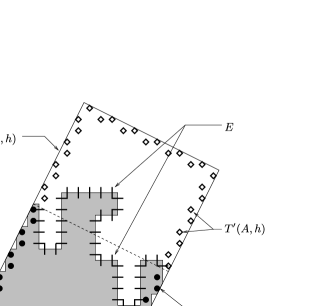
Figure 11: A $(B^{\prime}(A,h),T^{\prime}(A,h))$-cutset $E$ in $\operatorname{cyl}(A,h)$ and the corresponding set $S(E)$.

[this is a subset of $\mathbb{R}^{d}$ included in $\operatorname{cyl}(A,h)$; see Figure 11]. For each edge $e\in E$, $c(e)$ belongs to $\partial S(E)$ and the exterior unit vector normal to $S(E)$ at $c(e)$, which we denote by $\vec{v}_{S(E)}(c(e))$, is equal to $\vec{e}$ or $-\vec{e}$, thus $\vec{e}\cdot\vec{v}_{S(E)}(c(e))$ equals $+1$ or $-1$. If $\vec{e}\cdot\vec{v}_{S(E)}(c(e))=+1$ (resp., $-1$), then $\mathbf{e}=\langle a,b\rangle$ with $a\in s(E)$ [resp., $b\in s(E)$] and $b$ in the connected component of $T^{\prime}(A,h)$ in $(\mathbb{Z}^{d}_{n},\mathbb{E}^{d}_{n}\setminus E)\cap\operatorname{cyl}(A,h)$ (resp., $a$ in this component). Indeed, $E$ is minimal thus if we remove $e$ from $E$ we create a path from $B^{\prime}(A,h)$ to $T^{\prime}(A,h)$ that contains $e$. By the node law, we know that $\Psi(\vec{\mu}_{n},\operatorname{cyl}(A,h),\vec{v})$ is equal to the flow that crosses $E$ according to $\vec{\mu}_{n}$, that is,

$$\Psi\bigl{(}\vec{\mu}_{n},\operatorname{cyl}(A,h),\vec{v}\bigr{)}=\sum_{e\in E}f_{n}(e)\vec{e}\cdot\vec{v}_{S(E)}\bigl{(}c(e)\bigr{)}.$$ (63)

We construct now several such cutsets inside $\operatorname{cyl}(A,h)$. By symmetry, we can suppose that all the coordinates of $\vec{v}$ are nonnegative. Let $x$ be the center of $A$. Let $u\in\mathbb{R}$. We define the hypersurface $\mathcal{P}(u)$ by

$$\mathcal{P}(u)=\bigl{\{}y\in\mathbb{R}^{d}|\overrightarrow{xy}\cdot\vec{v}=u-h\bigr{\}}.$$

For each edge $e$ such that $\mathbf{e}=\langle a,b\rangle$, we define $\tilde{e}=[a,b[$, the segment that includes $b$, the endpoint of $\mathbf{e}$, but excludes $a$, its origin. We define the set of edges $E_{n}(u)$ by

$$E_{n}(u)=\bigl{\{}e\in\mathbb{E}^{d}_{n}|e\subset\operatorname{cyl}(A,h)\mbox{ and }\tilde{e}\cap\mathcal{P}(u)\neq\varnothing\bigr{\}};$$

see Figure 12. We define also the set of edges $F_{n}$ by

$$F_{n}=\bigl{\{}e\in\mathbb{E}^{d}_{n}|e\subset\operatorname{cyl}(A,h)\cap\mathcal{V}_{2}\bigl{(}\operatorname{cyl}(\partial A,h),2d/n\bigr{)}\bigr{\}},$$

which is the set of the edges in $\operatorname{cyl}(A,h)$ that are near the faces of the cylinder that are normal to $A$, and the set $\widetilde{E}_{n}(u)$ by

$$\widetilde{E}_{n}(u)=\bigl{\{}e\in E_{n}(u)|e\not\subset\mathcal{V}_{2}\bigl{(}\operatorname{cyl}(\partial A,h),4d/n\bigr{)}\bigr{\}},$$

which is the set of the edges of $E_{n}(u)$ that are not too close from the faces of the cylinder that are normal to $A$.

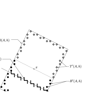
Figure 12: The set $E_{n}(u)$.

We need the following property:

Proposition 4.6

For all $u\in[1/n,2h-1/n]$, $E_{n}(u)\cup F_{n}$ contains a $(B^{\prime}(A,h),T^{\prime}(A,h))$-cutset in $\operatorname{cyl}(A,h)$. We denote such a cutset by $\widehat{E}_{n}(u)$. Necessarily $\widetilde{E}_{n}(u)$ is included in $\widehat{E}_{n}(u)$ (whichever way we construct it), and

$$\forall e\in\widetilde{E}_{n}(u)\qquad\vec{e}\cdot\vec{v}_{S(\widehat{E}_{n}(u))}\bigl{(}c(e)\bigr{)}=+1.$$

We consider such a cutset $\widehat{E}_{n}(u)$ for a given $u$ in $[1/n,2h-1/n]$. Using equation (63) we obtain as in Section 4.2 that

$$\biggl{|}\Psi\bigl{(}\vec{\mu}_{n},\operatorname{cyl}(A,h),\vec{v}\bigr{)}-\sum_{e\in E_{n}(u)}f_{n}(e)\biggr{|}$$

$$\qquad=\biggl{|}\sum_{e\in\widehat{E}_{n}(u)}f_{n}(e)\vec{e}\cdot\vec{v}_{S(\widehat{E}_{n}(u))}\bigl{(}c(e)\bigr{)}-\sum_{e\in E_{n}(u)}f_{n}(e)\biggr{|}$$

$$\qquad=\biggl{|}\sum_{e\in\widehat{E}_{n}(u)\setminus\widetilde{E}_{n}(u)}f_{n}(e)\vec{e}\cdot\vec{v}_{S(\widehat{E}_{n}(u))}\bigl{(}c(e)\bigr{)}-\sum_{e\in E_{n}(u)\setminus\widetilde{E}_{n}(u)}f_{n}(e)\biggr{|}$$

(64)

$$\qquad\leq M\bigl{[}\operatorname{card}\bigl{(}\widehat{E}_{n}(u)\setminus\widetilde{E}_{n}(u)\bigr{)}+\operatorname{card}\bigl{(}E_{n}(u)\setminus\widetilde{E}_{n}(u)\bigr{)}\bigr{]}$$

$$\qquad\leq 4dM\operatorname{card}\bigl{(}\mathbb{Z}^{d}_{n}\cap\mathcal{V}_{2}\bigl{(}\operatorname{cyl}(\partial A,h),4dn^{-1}\bigr{)}\bigr{)}$$

$$\qquad\leq 4dMn^{d}\mathcal{L}^{d}\bigl{(}\mathcal{V}_{2}\bigl{(}\operatorname{cyl}(\partial A,h),5dn^{-1}\bigr{)}\bigr{)}\leq CM\mathcal{H}^{d-2}(\partial A)\bigl{(}h+5dn^{-1}\bigr{)}n^{d-1}$$

for a constant $C$. Let us consider the quantity

$$\gamma=\int_{0}^{2h}\biggl{(}\sum_{e\in E_{n}(u)}f_{n}(e)\biggr{)}\,du.$$

On one hand, inequality (4.5) states that

$$\bigl{|}2h\Psi\bigl{(}\vec{\mu}_{n},\operatorname{cyl}(A,h),\vec{v}\bigr{)}-\gamma\bigr{|}$$

$$\qquad\leq 2hCM\mathcal{H}^{d-2}(\partial A)\bigl{(}h+5dn^{-1}\bigr{)}n^{d-1}$$

$$\qquad\quad{}+\int_{[0,1/n]\cup[2h-1/n,2h]}\biggl{|}\sum_{e\in E_{n}(u)}f_{n}(e)-\Psi\bigl{(}\vec{\mu}_{n},\operatorname{cyl}(A,h),\vec{v}\bigr{)}\biggr{|}\,du.$$

Moreover, there exists a constant $C^{\prime}(d,A)$ such that

$$\forall u\in\mathbb{R}\qquad\operatorname{card}\bigl{(}E_{n}(u)\bigr{)} \leq C^{\prime}(d,A)n^{d-1}\quad\mbox{and}$$

$$\bigl{|}\psi\bigl{(}\vec{\mu}_{n},\operatorname{cyl}(A,h),\vec{v}\bigr{)}\bigr{|} \leq C^{\prime}(d,A)Mn^{d-1}.$$

We obtain the second inequality by noticing that the set of edges $E_{n}(h)$ separates $B^{\prime}(A,h)$ from $T^{\prime}(A,h)$ in $\operatorname{cyl}(A,h)$, and the first inequality bounds its cardinal. We conclude that

$$\bigl{|}2h\Psi\bigl{(}\vec{\mu}_{n},\operatorname{cyl}(A,h),\vec{v}\bigr{)}-\gamma\bigr{|}$$

$$\qquad\leq 2CMh\bigl{(}h+5dn^{-1}\bigr{)}\mathcal{H}^{d-2}(\partial A)n^{d-1}+4C^{\prime}(d,A)Mn^{d-2}$$ (65)

$$\qquad\leq 2CMh^{2}\mathcal{H}^{d-2}(\partial A)n^{d-1}+K_{1}(d,A,h,M)n^{d-2}.$$

On the other hand, we have

$$\gamma=\sum_{e\in\operatorname{cyl}(A,h)}f_{n}(e)\int_{0}^{2h}\mathbh{1}_{\{e\in E_{n}(u)\}}\,du.$$

For all $e\in\operatorname{cyl}(A,h)$, $e\notin E_{n}(u)$ if $u\notin[0,2h]$, and we have

$$\int_{0}^{2h}\mathbh{1}_{\{e\in E_{n}(u)\}}\,du=\int_{\mathbb{R}}\mathbh{1}_{\{e\in E_{n}(u)\}}\,du=\frac{1}{n}\vec{e}\cdot\vec{v}.$$

Indeed for all $e\in\operatorname{cyl}(A,h)$, if $\mathbf{e}=\langle a,b\rangle$, then $\overrightarrow{xa}\cdot\vec{v}\leq\overrightarrow{xb}\cdot\vec{v}$ (remember that we supposed that the coordinates of $\vec{v}$ are non negative) and

$$e\in E_{n}(u)\quad\iff\quad\overrightarrow{xa}\cdot\vec{v}<u-h\leq\overrightarrow{xb}\cdot\vec{v}\quad\iff\quad u\in\,]h+\overrightarrow{xa}\cdot\vec{v},h+\overrightarrow{xb}\cdot\vec{v}],$$

and the measure of the above interval is

$$\overrightarrow{xb}\cdot\vec{v}-\overrightarrow{xa}\cdot\vec{v}=\frac{1}{n}\vec{e}\cdot\vec{v}.$$

Thus

$$\biggl{|}\gamma-n^{d-1}\int_{\operatorname{cyl}(A,h)}\,d\vec{\mu}_{n}\cdot\vec{v}\biggr{|}$$

$$\qquad=\biggl{|}\frac{1}{n}\sum_{e\in\operatorname{cyl}(A,h)}f_{n}(e)\vec{e}\cdot\vec{v}-\frac{1}{n}\mathop{\sum_{e\in\mathbb{E}^{d}_{n},}}_{c(e)\in\operatorname{cyl}(A,h)}f_{n}(e)\vec{e}\cdot\vec{v}\biggr{|}$$

(66)

$$\qquad\leq\frac{M}{n}\operatorname{card}\bigl{(}\bigl{\{}e\in\mathbb{E}^{d}_{n}|e\cap\partial\operatorname{cyl}(A,h)\neq\varnothing\bigr{\}}\bigr{)}$$

$$\qquad\leq K_{2}(d,A,h,M)n^{d-2}.$$

Combining inequalities (4.5) and (4.5) we obtain

$$\biggl{|}\int_{\operatorname{cyl}(A,h)}\,d\vec{\mu}_{n}\cdot\vec{v}-\frac{2h\Psi(\vec{\mu}_{n},\operatorname{cyl}(A,h),\vec{v})}{n^{d-1}}\biggr{|}$$

$$\qquad\leq 2CMh^{2}\mathcal{H}^{d-2}(\partial A)+\bigl{(}K_{1}(d,A,h,M)+K_{2}(d,A,h,M)\bigr{)}n^{-1}.$$

We define

$$h_{0}(A,\eta)=\frac{\eta\mathcal{H}^{d-1}(A)}{4CM\mathcal{H}^{d-2}(\partial A)}.$$

We deduce from inequality (4.5) that all $h\leq h_{0}$, for all $n$ we have

$$\biggl{|}\int_{\operatorname{cyl}(A,h)}\,d\vec{\mu}_{n}\cdot\vec{v}-\frac{2h\Psi(\vec{\mu}_{n},\operatorname{cyl}(A,h),\vec{v})}{n^{d-1}}\biggr{|}$$

$$\qquad\leq\frac{\eta\mathcal{L}^{d}(\operatorname{cyl}(A,h))}{2}+\bigl{(}K_{1}(A,h,M)+K_{2}(A,h,M)\bigr{)}n^{-1},$$

and thus for $n$ large enough (how large depending on $A,h,M$) we obtain the desired inequality. Moreover for all $\varepsilon>0$, $y\in\mathbb{R}^{d}$, we immediatly obtain that

$$h_{0}(y+\varepsilon A,\eta)=\frac{\eta\mathcal{H}^{d-1}(y+\varepsilon A)}{4CM\mathcal{H}^{d-2}(\partial(y+\varepsilon A))}=\frac{\eta\varepsilon^{d-1}\mathcal{H}^{d-1}(A)}{4CM\varepsilon^{d-2}\mathcal{H}^{d-2}(\partial A)}=\varepsilon h_{0}(A,\eta).$$

This ends the proof of Proposition 4.5.

Proof of Proposition 4.6 First of all, we prove that for all $u\in[1/n,2h-1/n]$, $E_{n}(u)$ separates the bottom from the top of $\operatorname{cyl}(A,h)$. Let us consider a self-avoiding path $r$ from $B(A,h)$ to $T(A,h)$ in $\operatorname{cyl}(A,h)$. The path $r$ admits a continuous parametrization $r=(r_{t})_{t\in[0,1]}$. Let $x$ be the center of $A$. The two sets

$$V_{1}(u) = \bigl{\{}y\in\mathbb{R}^{d}|\overrightarrow{xy}\cdot\vec{v}<u-h\bigr{\}}\cap\operatorname{cyl}(A,h),$$

$$V_{2}(u) = \bigl{\{}y\in\mathbb{R}^{d}|\overrightarrow{xy}\cdot\vec{v}\geq u-h\bigr{\}}\cap\operatorname{cyl}(A,h)$$

form a partition of $\operatorname{cyl}(A,h)$. The path $r$ starts in $V_{1}(u)$ and ends in $V_{2}(u)$. Indeed, $B(A,h)\subset\mathcal{V}_{2}(A-h\vec{v},n^{-1})\subset V_{1}(u)$ because $u\geq n^{-1}$ and $T(A,h)\subset\mathcal{V}_{2}(A+h\vec{v},n^{-1})\subset V_{2}(u)$ because $u\leq 2h-n^{-1}$. Since $r$ is continuous, there exists $t_{0}\in[0,1]$ such that

$$t_{0}=\sup\bigl{\{}t\in[0,1]|r_{t}\in V_{1}(u)\bigr{\}}.$$

We define the point $z=r_{t_{0}}$. It is obvious that $z\in\mathcal{P}(u)$; see Figure 13. If $z\notin\mathbb{Z}^{d}_{n}$, then $z$ belongs only to one edge $e\subset r\subset\operatorname{cyl}(A,h)$, and $z$ is not an extreme point of $e$ so $z\in\mathcal{P}(u)$ implies that $e\in E_{n}(u)$. If $z\in\mathbb{Z}^{d}_{n}$, then $z$ belongs to exactly two edges $e_{1}$ and $e_{2}$ that are included in $r$. By the definition of $t_{0}$, we know that one of these edges, say $e_{1}$ for example, is included in the adherence of $V_{1}(u)$, and the other one, $e_{2}$, is included in $V_{2}(u)$. Since all the coordinates of $\vec{v}$ are nonnegative, we conclude that $e_{2}\in E_{n}(u)$. This proves that $E_{n}(u)$ separates $T(A,h)$ from $B(A,h)$ in $\operatorname{cyl}(A,h)$.

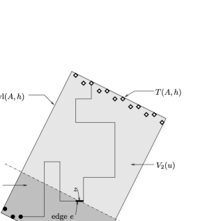
Figure 13: The set $E_{n}(u)$ separates $B(A,h)$ from $T(A,h)$ in $\operatorname{cyl}(A,h)$.

We deduce easily that $E_{n}(u)\cup F_{n}$ separates $T^{\prime}(A,h)$ from $B^{\prime}(A,h)$ in $\operatorname{cyl}(A,h)$. Indeed, consider a path $\hat{r}$ from $T^{\prime}(A,h)$ to $B^{\prime}(A,h)$ in $\operatorname{cyl}(A,h)$. If the starting point (resp., the endpoint) of $\hat{r}$ belongs to $T^{\prime}(A,h)\setminus T(A,h)$ [resp., $B^{\prime}(A,h)\setminus B(A,h)$], then the first (resp., last) edge of $r$ belongs to $F_{n}$. Otherwise, $\hat{r}$ is a path from $T(A,h)$ to $B(A,h)$ in $\operatorname{cyl}(A,h)$, and we have proved that it must contain at least one edge of $E_{n}(u)$.

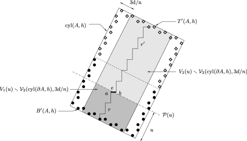
Figure 14: Construction of a path from $B(A,h)$ to $T(A,h)$.

We consider an edge $e$ of $\widetilde{E}_{n}(u)$, $\mathbf{e}=\langle a,b\rangle$. Then $a\in V_{1}(u)$ and $b\in V_{2}(u)$. Moreover $e\not\subset\mathcal{V}_{2}(\operatorname{cyl}(\partial A,h),4d/n)$ implies that $d_{2}(a,\operatorname{cyl}(\partial A,h))>3d/n$. The set

$$\mathcal{D}=V_{1}(u)\setminus\mathcal{V}_{2}\bigl{(}\operatorname{cyl}(\partial A,h),3d/n\bigr{)}$$

is a parallelepiped; thus the graph $\mathcal{D}\cap(\mathbb{Z}^{d}_{n},\mathbb{E}^{d}_{n})$ is connected. Let $r$ be a path from $a$ to $B(A,h)$ included in $\mathcal{D}$; see Figure 14. In the same way, there exists a path $r^{\prime}$ from $b$ to $T(A,h)$ that is included in $V_{2}(u)\setminus\mathcal{V}_{2}(\operatorname{cyl}(\partial A,h),3d/n)$. Thus $r\cup e\cup r^{\prime}$ is a path from $B(A,h)$ to $T(A,h)$ that does not contain edges of $F_{n}\cup(E_{n}(u)\setminus\{e\})$, and we conclude that $F_{n}\cup(E_{n}(u)\setminus\{e\})$ does not separate $B(A,h)$ from $T(A,h)$ in $\operatorname{cyl}(A,h)$. This implies that $e$ must belong to any cutset $\widehat{E}_{n}(u)$ with the properties given in Proposition 4.6. Moreover, we have proved that $a\in S(\widehat{E}_{n}(u))$ and $b\notin S(\widehat{E}_{n}(u))$, and this implies that $\vec{v}_{S(\widehat{E}_{n}(u))}(c(e))=\vec{e}$, so Proposition 4.6 is proved.

4.6 Maximality

We recall that

$$\operatorname{flow}^{\mathrm{cont}}(\vec{\sigma})=\int_{\Gamma^{1}}-\vec{\sigma}\cdot\vec{v}_{\Omega}\,d\mathcal{H}^{d-1}$$

and

$$\operatorname{flow}^{\mathrm{disc}}_{n}(\vec{\mu}_{n})=\frac{1}{n^{d-1}}\sum_{e\in\Pi_{n}:e=[ab],a\in\Gamma^{1}_{n},b\notin\Gamma^{1}_{n}}f_{n}(e)(\mathbh{1}_{\{\mathbf{e}=\langle a,b\rangle\}}-\mathbh{1}_{\{\mathbf{e}=\langle b,a\rangle\}}).$$

To complete the proof of Theorem 1.1, we must prove that the limit $\vec{\mu}=\vec{\sigma}\mathcal{L}^{d}$ of a subsequence of the sequence of maximal discrete flows $(\vec{\mu}_{n}^{\max})_{n\geq 1}$ satisfies

$$\operatorname{flow}^{\mathrm{cont}}(\vec{\sigma})=\phi_{\Omega}^{b}\qquad\mbox{a.s.}$$ (68)

In this section, we prove the following result:

Proposition 4.7

Let $(\vec{\mu}_{n})_{n\geq 1}$ be a sequence of admissible discrete streams. If a subsequence $(\vec{\mu}_{\varphi(n)})_{n\geq 1}$ converges weakly toward a measure $\vec{\mu}=\vec{\sigma}\mathcal{L}^{d}$ with $\vec{\sigma}\in L^{\infty}(\mathbb{R}^{d}\rightarrow\mathbb{R}^{d},\mathcal{L}^{d})$, then

$$\lim_{n\rightarrow\infty}\operatorname{flow}^{\mathrm{disc}}_{\varphi(n)}(\vec{\mu}_{\varphi(n)})=\operatorname{flow}^{\mathrm{cont}}(\vec{\sigma}).$$

Remark 14.

We will deduce equation (68) from Proposition 4.7 in Section 6, using our study of minimal cutsets and Lemma 1.

Proof of Proposition 4.7 The idea of the proof is very similar to the one of Proposition 4.4. Suppose $\vec{\sigma}$ is very regular—$\mathcal{C}^{1}$ for example. By the Gauss–Green theorem, we know that for all sets $E$ with finite perimeter,

$$\int_{\partial E}\vec{\sigma}\cdot\vec{v}_{E}\,d\mathcal{H}^{d-1}=\int_{E}\operatorname{div}\vec{\sigma}\,d\mathcal{L}^{d}=0.$$

If $\partial E=\Gamma^{1}\cup\mathcal{S}\cup\widehat{\mathcal{S}}$, where $\widehat{\mathcal{S}}\subset\Gamma\setminus(\Gamma^{1}\cup\Gamma^{2})$ and $\mathcal{S}=\partial E\cap\Omega$, then we obtain

$$\int_{\mathcal{S}}\vec{\sigma}\cdot\vec{v}_{E}\,d\mathcal{H}^{d-1}=-\int_{\Gamma^{1}}\vec{\sigma}\cdot\vec{v}_{\Omega}\,d\mathcal{H}^{d-1}+0=\operatorname{flow}^{\mathrm{cont}}(\vec{\sigma}).$$

We can choose $E$ such that $\mathcal{S}$ is polyhedral: it allows us to cover (up to a small volume) a neighborhood of $\mathcal{S}$ by a union of cylinders $D_{i}$ of height $h$ and oriented in the direction $\vec{v}_{i}$, where $\vec{v}_{i}=\vec{v}_{E}$ on the face of $\mathcal{S}$ that $D_{i}$ crosses. As explained in the sketch of the proof of Proposition 4.4, $\int_{D_{i}}\vec{\sigma}\cdot\vec{v}_{i}\,d\mathcal{H}^{d-1}$ is very close to $h\int_{\mathcal{S}\cap D_{i}}\vec{\sigma}\cdot\vec{v}_{i}\,d\mathcal{H}^{d-1}$. Since $\vec{\mu}_{n}\rightharpoonup\vec{\sigma}\mathcal{L}^{d}$, $\int_{D_{i}}\vec{\sigma}\cdot\vec{v}_{i}\,d\mathcal{L}^{d}$ is the limit of $\int_{D_{i}}\,d\vec{\mu}_{n}\cdot\vec{v}_{i}$. By Proposition 4.5, we know that $\int_{D_{i}}\,d\vec{\mu}_{n}\cdot\vec{v}_{i}$ is very close to $\Psi(\vec{\mu}_{n},D_{i},\vec{v}_{i})$. Finally, we notice that the flow that crosses $\Omega_{n}$ from $\Gamma^{1}_{n}$ to $\Gamma^{2}_{n}$ is the flow that crosses the $D_{i}$ up to a small error, and thus $\operatorname{flow}^{\mathrm{disc}}_{n}(\vec{\mu}_{n})$ is close to $\sum_{i}\Psi(\vec{\mu}_{n},D_{i},\vec{v}_{i})$ properly rescaled. This is exactly the idea we follow to compare $\operatorname{flow}^{\mathrm{disc}}_{n}(\vec{\mu}_{n})$ to $\operatorname{flow}^{\mathrm{cont}}(\vec{\sigma})$. However, $\vec{\sigma}$ is not regular enough to allow a direct application of the Gauss–Green theorem. The easiest way to get round this problem is to come back to the definition of the divergence $\operatorname{div}\vec{\sigma}$ to compare $\operatorname{flow}^{\mathrm{cont}}(\vec{\sigma})$ to a sum of the type $\sum_{i}\int_{D_{i}}\vec{\sigma}\cdot\vec{v}_{i}\,d\mathcal{L}^{d}$.

From now on we consider a fixed realization of the capacities. We consider a subsequence of $(\vec{\mu}_{n})_{n\geq 1}$ converging toward $\vec{\mu}$, but we still denote this subsequence by $(\vec{\mu}_{n})_{n\geq 1}$ to simplify the notation.

Step 1: From $\operatorname{flow}^{\mathrm{cont}}(\vec{\sigma})$ to $\sum_{i=1}^{\mathcal{N}}\int_{\operatorname{cyl}(A_{i},h)}\vec{\sigma}\cdot\vec{v}_{i}\,d\mathcal{L}^{d}$. For $\mathcal{A}$ a subset of $\mathbb{R}^{d}$, we denote by $\overline{\mathcal{A}}$ its closure and by $\stackrel{{\scriptstyle\circ}}{{\mathcal{A}}}$ its interior. Let $P$ be a closed polyhedral set of $\mathbb{R}^{d}$ such that

$$\overline{\Gamma}^{1}\subset\stackrel{{\scriptstyle\circ}}{{P}},\qquad\overline{\Gamma}^{2}\subset\,\stackrel{{\scriptstyle\circ}}{{\wideparen{\mathbb{R}^{d}\setminus P}}}\quad\mbox{and}\quad\partial P\mbox{ is transversal to }\Gamma.$$

The construction of such a set $P$ is made in Section 5 of CerfTheret09supc . The idea of the construction is the following. For each $x\in\overline{\Gamma}^{1}$, let $C_{x}$ be a closed cube of center $x$ and of positive size but small enough so that $d_{2}(C_{x},\Gamma^{2})\geq d_{2}(\Gamma^{1},\Gamma^{2})/2$. The cubes $(C_{x})_{x\in\overline{\Gamma}^{1}}$ can be chosen carefully so that their boundaries are transversal to $\Gamma$. Of course,

$$\overline{\Gamma}^{1}\subset\bigcup_{x\in\overline{\Gamma}^{1}}\stackrel{{\scriptstyle\circ}}{{C}}_{x},$$

and by compactness of $\overline{\Gamma}^{1}$ we know that there exists a finite subcovering of $\overline{\Gamma}^{1}$, say

$$\overline{\Gamma}^{1}\subset\bigcup_{i=1}^{p}\stackrel{{\scriptstyle\circ}}{{C}}_{x_{i}}.$$

We can take $P=\bigcup_{i=1}^{p}C_{x_{i}}$. By construction $\partial P$ is a polyhedral hypersurface that is transversal to $\Gamma$ and that does not intersect $\overline{\Gamma}^{1}$ nor $\overline{\Gamma}^{2}$, thus $d_{2}(\partial P,\Gamma^{1}\cup\Gamma^{2})>0$. In the same way, for any $\zeta>0$, we can construct a set $\Omega^{\prime}$ satisfying $\Omega\subset\Omega^{\prime}\subset\mathcal{V}_{2}(\Omega,\zeta)$ and such that $\partial\Omega^{\prime}$ is polyhedral and transversal to $\partial P$. We fix a positive real number $\widehat{\eta}>0$. Since $\partial P$ is transversal to $\Gamma$, there exists $\varepsilon(\widehat{\eta})>0$ such that $\mathcal{H}^{d-1}(\partial P\cap(\mathcal{V}_{2}(\Omega,\varepsilon)\setminus\Omega))\leq\widehat{\eta}$. We consider a set $\Omega^{\prime}$ corresponding to $\varepsilon(\widehat{\eta})$ as described previously. Thus $\Omega^{\prime}$ depends on $\Omega$, $P$ and $\widehat{\eta}$, and we have

$$\mathcal{H}^{d-1}\bigl{(}\partial P\cap\bigl{(}\Omega^{\prime}\setminus\Omega\bigr{)}\bigr{)}\leq\widehat{\eta}.$$ (69)

We need the following property (see Figure 15):

Figure 15: The cylinders $(\operatorname{cyl}(A_{i},h),i=1,\ldots,\mathcal{N})$.

Proposition 4.8

Let $\eta>0$. There exists a finite family of hyperrectangles $A_{1},\ldots,A_{\mathcal{N}}$ (depending on $\Omega,P,\widehat{\eta},\eta$) of disjoint interiors included in $\partial P\cap\Omega^{\prime}$, a positive real number $h_{1}(\Omega,P,\eta,\widehat{\eta})$ and a constant $C(\Omega,P,\widehat{\eta})$ such that for all $h\leq h_{1}$, we have:

• $\mathcal{H}^{d-1}((\partial P\cap\Omega^{\prime})\setminus(\bigcup_{i=1}^{\mathcal{N}}A_{i}))\leq\eta$;

• $\mathcal{L}^{d}((\mathcal{V}_{2}(\partial P,h)\cap\Omega^{\prime})\setminus\bigcup_{i=1}^{\mathcal{N}}\operatorname{cyl}(A_{i},h))\leq 2C\eta h$;

• $\forall i\in\{1,\ldots,\mathcal{N}\},\operatorname{cyl}(A_{i},h)\subset\Omega^{\prime}$;

• $\forall i\in\{1,\ldots,\mathcal{N}\},\forall x\in\operatorname{cyl}(A_{i},h),d_{2}(x,\partial P\setminus A_{i})>d_{2}(x,A_{i})$.

We admit this proposition for the time being. We fix a positive $\eta$. For each $i\in\{1,\ldots,\mathcal{N}\}$, let $\vec{v}_{i}$ be the exterior normal unit vector to $P$ along the face of $\partial P$ on which $A_{i}$ is, thus $\vec{v}_{i}$ is normal to $A_{i}$. We have explained in Remark 13 that $\operatorname{div}\vec{\sigma}\mathcal{L}^{d}=-(\vec{\sigma}\cdot\vec{v}_{\Omega})\mathcal{H}^{d-1}|_{\Gamma}$. Thus for any function $\varphi\in W^{1,1}(\mathbb{R}^{d})$, we have

$$\int_{\Omega}\vec{\sigma}\cdot\vec{\nabla}\varphi\,d\mathcal{L}^{d} = \int_{\mathbb{R}^{d}}\vec{\sigma}\cdot\vec{\nabla}\varphi\,d\mathcal{L}^{d}=-\int_{\mathbb{R}^{d}}\varphi\operatorname{div}\vec{\sigma}\,d\mathcal{L}^{d}$$

$$= +\int_{\Gamma}(\vec{\sigma}\cdot\vec{v}_{\Omega})\gamma(\varphi|_{\Omega})\,d\mathcal{H}^{d-1}$$

(this corresponds exactly to the definition of $\vec{\sigma}\cdot\vec{v}_{\Omega}$ given in Nozawa ; cf. equation (49)). For a positive $h\leq h_{1}$, we define the function $\varphi_{h}$ by

$$\varphi_{h}(x)=\zeta\biggl{(}\frac{d_{2}(x,P^{c})}{h}\biggr{)}+\zeta\biggl{(}\frac{h-d_{2}(x,P)}{h}\biggr{)},$$

where $\zeta(r)=r\mathbh{1}_{[0,1[}+\mathbh{1}_{[1,+\infty[}$. Then $\varphi_{h}=2$ on $P\cap\mathcal{V}_{2}(\partial P,h)^{c}$ and $\varphi_{h}=0$ on $P^{c}\cap\mathcal{V}_{2}(\partial P,h)^{c}$, $\varphi_{h}$ is Lipschitz and has compact support included in $P\cup\mathcal{V}_{2}(\partial P,h)$, in particular $\varphi_{h}\in W^{1,1}(\mathbb{R}^{d})$. On one hand, we know that $\vec{\sigma}\cdot\vec{v}_{\Omega}=0$ $\mathcal{H}^{d-1}$-a.e. on $\Gamma\setminus(\Gamma^{1}\cup\Gamma^{2})$, and there exists $h_{2}(\Omega,P)=d_{2}(\partial P,\Gamma^{1}\cup\Gamma^{2})/2>0$ such that for $h\leq h_{2}$ we have $\gamma(\varphi_{h}|_{\Omega})=\varphi_{h}=2$ $\mathcal{H}^{d-1}$-a.e. on $\Gamma^{1}$ and $\gamma(\varphi_{h}|_{\Omega})=\varphi_{h}=0$ $\mathcal{H}^{d-1}$-a.e. on $\Gamma^{2}$, thus

$$\int_{\Gamma}(\vec{\sigma}\cdot\vec{v}_{\Omega})\gamma(\varphi_{h}|_{\Omega})\,d\mathcal{H}^{d-1}=2\int_{\Gamma^{1}}(\vec{\sigma}\cdot\vec{v}_{\Omega})\,d\mathcal{H}^{d-1}=-2\operatorname{flow}^{\mathrm{cont}}(\vec{\sigma}).$$

On the other hand, we know that

$$\vec{\nabla}\varphi_{h}(\cdot)=\mathbh{1}_{[0,1[}\biggl{(}\frac{d_{2}(\cdot,P^{c})}{h}\biggr{)}h^{-1}\vec{\nabla}d_{2}\bigl{(}\cdot,P^{c}\bigr{)}-\mathbh{1}_{[0,1[}\biggl{(}\frac{h-d_{2}(\cdot,P)}{h}\biggr{)}h^{-1}\vec{\nabla}d_{2}(\cdot,P),$$

thus $\vec{\nabla}\varphi_{h}=0$ $\mathcal{L}^{d}$-a.e. on $\mathcal{V}_{2}(\partial P,h)^{c}$, $\|\vec{\nabla}\varphi_{h}\|_{\infty}\leq h^{-1}$, and for all $i\in\{1,\ldots,\mathcal{N}\}$ we have on $\operatorname{cyl}(A_{i},h)$

$$\vec{\nabla}\varphi_{h}=-h^{-1}\vec{v}_{i}.$$

For all $h\leq\min(h_{1},h_{2})$, equation (4.6) applied to $\varphi_{h}$ gives

$$\operatorname{flow}^{\mathrm{cont}}(\vec{\sigma})$$

$$\qquad=-\frac{1}{2}\int_{\Gamma}(\vec{\sigma}\cdot\vec{v}_{\Omega})\gamma(\varphi_{h}|_{\Omega})\,d\mathcal{H}^{d-1}$$

$$\qquad=-\frac{1}{2}\int_{\Omega}\vec{\sigma}\cdot\vec{\nabla}\varphi_{h}\,d\mathcal{L}^{d}$$

$$\qquad=-\frac{1}{2}\int_{\mathcal{V}_{2}(\partial P,h)\cap\Omega}\vec{\sigma}\cdot\vec{\nabla}\varphi_{h}\,d\mathcal{L}^{d}$$

$$\qquad=-\frac{1}{2}\sum_{i=1}^{\mathcal{N}}\int_{\operatorname{cyl}(A_{i},h)}\vec{\sigma}\cdot\biggl{(}-\frac{1}{h}\vec{v}_{i}\biggr{)}\,d\mathcal{L}^{d}$$

$$\qquad\quad{}-\frac{1}{2}\int_{(\mathcal{V}_{2}(\partial P,h)\cap\Omega)\setminus\bigcup_{i=1}^{\mathcal{N}}\operatorname{cyl}(A_{i},h)}\vec{\sigma}\cdot\vec{\nabla}\varphi_{h}\,d\mathcal{L}^{d}.$$

Thus

$$\Biggl{|}\operatorname{flow}^{\mathrm{cont}}(\vec{\sigma})-\frac{1}{2h}\sum_{i=1}^{\mathcal{N}}\int_{\operatorname{cyl}(A_{i},h)}\vec{\sigma}\cdot\vec{v}_{i}\,d\mathcal{L}^{d}\Biggr{|}$$

$$\qquad\leq\frac{1}{2}\|\vec{\sigma}\|_{\infty}\|\vec{\nabla}\varphi_{h}\|_{\infty}\mathcal{L}^{d}\Biggl{(}\bigl{(}\mathcal{V}_{2}(\partial P,h)\cap\Omega\bigr{)}\setminus\bigcup_{i=1}^{\mathcal{N}}\operatorname{cyl}(A_{i},h)\Biggr{)}$$

(71)

$$\qquad\leq\frac{1}{2}\|\vec{\sigma}\|_{\infty}\|\vec{\nabla}\varphi_{h}\|_{\infty}\mathcal{L}^{d}\Biggl{(}\bigl{(}\mathcal{V}_{2}(\partial P,h)\cap\Omega^{\prime}\bigr{)}\setminus\bigcup_{i=1}^{\mathcal{N}}\operatorname{cyl}(A_{i},h)\Biggr{)}$$

$$\qquad\leq C\eta\|\vec{\sigma}\|_{\infty}.$$

Step 2: From $\int_{\operatorname{cyl}(A_{i},h)}\vec{\sigma}\cdot\vec{v}_{i}\,d\mathcal{L}^{d}$ to $\int_{\operatorname{cyl}(A_{i},h)}\,d\vec{\mu}_{n}\cdot\vec{v}_{i}$. As in Section 4.5 if $\vec{\mu}_{n}\rightharpoonup\vec{\sigma}\mathcal{L}^{d}$ (up to extraction), since $\mathcal{L}^{d}(\partial\operatorname{cyl}(A_{i},h))=0$, we know by Portmanteau theorem that for all $i\in\{1,\ldots,\mathcal{N}\}$, for all $n$ large enough (how large depending on $P,A_{i},h,\eta$) we have

$$\biggl{|}\int_{\operatorname{cyl}(A_{i},h)}\vec{\sigma}\cdot\vec{v}_{i}\,d\mathcal{L}^{d}-\int_{\operatorname{cyl}(A_{i},h)}\,d\vec{\mu}_{n}\cdot\vec{v}_{i}\biggr{|}\leq\frac{\eta h}{\mathcal{N}},$$

and we conclude that for all $n$ large enough (how large depending on $P,h,\eta$), we have

$$\Biggl{|}\sum_{i=1}^{\mathcal{N}}\int_{\operatorname{cyl}(A_{i},h)}\vec{\sigma}\cdot\vec{v}_{i}\,d\mathcal{L}^{d}-\sum_{i=1}^{\mathcal{N}}\int_{\operatorname{cyl}(A_{i},h)}\,d\vec{\mu}_{n}\cdot\vec{v}_{i}\Biggr{|}\leq\eta h.$$ (72)

Step 3: From $\int_{\operatorname{cyl}(A_{i},h)}\,d\vec{\mu}_{n}\cdot\vec{v}_{i}$ to $\Psi(\vec{\mu}_{n},\operatorname{cyl}(A_{i},h),\vec{v}_{i})$. As in Section 4.5 we use Proposition 4.5 to obtain that for all $i\in\{1,\ldots,\mathcal{N}\}$, there exists $\widetilde{h}_{i}(P,\eta)>0$ such that for all $h\leq\widetilde{h}_{i}$, for all $n$ large enough (how large depending on $P,h,\eta$), we have

$$\biggl{|}\int_{\operatorname{cyl}(A_{i},h)}\,d\vec{\mu}_{n}\cdot\vec{v}_{i}-\frac{2h\Psi(\vec{\mu}_{n},\operatorname{cyl}(A_{i},h),\vec{v}_{i})}{n^{d-1}}\biggr{|}\leq\frac{\eta}{\sum_{i=1}^{\mathcal{N}}\mathcal{H}^{d-1}(A_{i})}\mathcal{L}^{d}\bigl{(}\operatorname{cyl}(A_{i},h)\bigr{)}.$$

Thus there exists $h_{3}(P,\eta)=\min_{1\leq i\leq\mathcal{N}}(\widetilde{h}_{i})>0$ such that for all $h\leq h_{3}$, for all $n$ large enough (how large depending on $P,\eta$), we have

$$\Biggl{|}\sum_{i=1}^{\mathcal{N}}\int_{\operatorname{cyl}(A_{i},h)}\,d\vec{\mu}_{n}\cdot\vec{v}_{i}-\frac{2h}{n^{d-1}}\sum_{i=1}^{\mathcal{N}}\Psi\bigl{(}\vec{\mu}_{n},\operatorname{cyl}(A_{i},h),\vec{v}_{i}\bigr{)}\Biggr{|}\leq\eta h.$$ (73)

Step 4: From $\sum_{i=1}^{\mathcal{N}}\Psi(\vec{\mu}_{n},\operatorname{cyl}(A_{i},h),\vec{v}_{i})$ to $\operatorname{flow}^{\mathrm{disc}}_{n}(\vec{\mu}_{n})$. By construction of $P$ we know that $\Gamma^{1}_{n}\subset P$ and $\Gamma_{n}^{2}\subset(\mathbb{R}^{d}\setminus P)$ at least for $n$ large enough. Since the stream $f_{n}$ satisfies the node law, we know that $\operatorname{flow}^{\mathrm{disc}}_{n}(\vec{\mu}_{n})$ is equal to the flow that goes out of $P$, that is,

$$\operatorname{flow}^{\mathrm{disc}}_{n}(\vec{\mu}_{n})=\frac{1}{n^{d-1}}\sum_{e=[a,b],a\in P,b\notin P}f_{n}(e)\vec{e}\cdot(n\overrightarrow{ab}).$$

Notice that $\vec{e}\cdot(n\overrightarrow{ab})$ equals $+1$ or $-1$, and $f_{n}(e)=0$ if $e\notin\Pi_{n}$. We define

$$E(P)=\bigl{\{}e=[a,b]|e\in\Pi_{n},a\in P,b\notin P\bigr{\}}.$$

Thus

$$\operatorname{flow}^{\mathrm{disc}}_{n}(\vec{\mu}_{n})=\frac{1}{n^{d-1}}\sum_{e\in E(P)}f_{n}(e)\vec{e}\cdot(n\overrightarrow{ab}).$$

For all $i\in\{1,\ldots,\mathcal{N}\}$, for all $h>0$, the set of edges

$$E_{i}=\bigl{\{}e\subset\operatorname{cyl}(A_{i},h)|e\in E(P)\bigr{\}}$$

is a cutset in $\operatorname{cyl}(A_{i},h)$ from the lower half part of its boundary to the upper half part of its boundary in the direction $\vec{v}_{i}$; this can be proved exactly as in Proposition 4.6. Thus

$$\Psi\bigl{(}\vec{\mu}_{n},\operatorname{cyl}(A_{i},h),\vec{v}_{i}\bigr{)}=\sum_{e=[a,b]\in E_{i},a\in P,b\notin P}f_{n}(e)\vec{e}\cdot(n\overrightarrow{ab}).$$

Since the sets $E_{i}$ are disjoint, this implies that

$$\Biggl{|}\operatorname{flow}^{\mathrm{disc}}_{n}(\vec{\mu}_{n})-\frac{1}{n^{d-1}}\sum_{i=1}^{\mathcal{N}}\Psi\bigl{(}\vec{\mu}_{n},\operatorname{cyl}(A_{i},h),\vec{v}_{i}\bigr{)}\Biggr{|}\leq\frac{M}{n^{d-1}}\operatorname{card}\Biggl{(}E(P)\setminus\bigcup_{i=1}^{\mathcal{N}}E_{i}\Biggr{)}.$$

It remains to control $\operatorname{card}(E(P)\setminus\bigcup_{i=1}^{\mathcal{N}}E_{i})$. The edges that belong to this set are included in $\mathcal{V}_{\infty}((\partial P\cap\Omega^{\prime})\setminus\bigcup_{i=1}^{\mathcal{N}}A_{i},2/n)$, thus

$$\operatorname{card}\Biggl{(}E(P)\setminus\bigcup_{i=1}^{\mathcal{N}}E_{i}\Biggr{)} \leq 2d\operatorname{card}\Biggl{(}\mathcal{V}_{\infty}\Biggl{(}\bigl{(}\partial P\cap\Omega^{\prime}\bigr{)}\setminus\bigcup_{i=1}^{\mathcal{N}}A_{i},2/n\Biggr{)}\cap\mathbb{Z}^{d}_{n}\Biggr{)}$$

$$\leq 2dn^{d}\mathcal{L}^{d}\Biggl{(}\mathcal{V}_{\infty}\Biggl{(}\overline{\bigl{(}\partial P\cap\Omega^{\prime}\bigr{)}\setminus\bigcup_{i=1}^{\mathcal{N}}A_{i}},3/n\Biggr{)}\Biggr{)}.$$

The set $\overline{(\partial P\cap\Omega^{\prime})\setminus\bigcup_{i=1}^{\mathcal{N}}A_{i}}$ is a closed $(d-1)$-rectifiable set. Thus its $(d-1)$ dimensional Minkowski content defined by

$$\lim_{r\rightarrow 0}\frac{1}{2r}\mathcal{L}^{d}\Biggl{(}\mathcal{V}_{2}\Biggl{(}\overline{\bigl{(}\partial P\cap\Omega^{\prime}\bigr{)}\setminus\bigcup_{i=1}^{\mathcal{N}}A_{i}},r\Biggr{)}\Biggr{)}$$

exists and is equal to $\mathcal{H}^{d-1}(\overline{(\partial P\cap\Omega^{\prime})\setminus\bigcup_{i=1}^{\mathcal{N}}A_{i}})$ that is smaller than $\eta$ by construction. Thus there exists a constant $\kappa(d)$ such that, for $n$ large enough,

$$\operatorname{card}\Biggl{(}E(P)\setminus\bigcup_{i=1}^{\mathcal{N}}E_{i}\Biggr{)}\leq\kappa\eta n^{d-1}.$$

For all $n$ large enough we get

$$\Biggl{|}\operatorname{flow}^{\mathrm{disc}}_{n}(\vec{\mu}_{n})-\frac{1}{n^{d-1}}\sum_{i=1}^{\mathcal{N}}\Psi\bigl{(}\vec{\mu}_{n},\operatorname{cyl}(A_{i},h),\vec{v}_{i}\bigr{)}\Biggr{|}\leq\kappa\eta M.$$ (74)

Step 5: Conclusion. Combining inequalities (4.6), (72), (73) and (74) for a $h\leq\min(h_{1},h_{2},h_{3})$, we obtain that for all $n$ large enough (how large depending on everything else)

$$\bigl{|}\operatorname{flow}^{\mathrm{cont}}(\vec{\sigma})-\operatorname{flow}^{\mathrm{disc}}_{n}(\vec{\mu}_{n})\bigr{|}\leq\eta\bigl{(}C\|\vec{\sigma}\|_{\infty}+1+\kappa M\bigr{)},$$

and this completes the proof of Proposition 4.7.

Proof of Proposition 4.8 Let $\eta>0$. The sets $P$ and $\Omega^{\prime}$ are polyhedral; that is, their boundaries are included in a finite number of hyperplanes. For any $x\in\partial P\cap\partial\Omega^{\prime}$, let us denote by $\theta(x)\in[0,\pi]$ the angle between the exterior unit normal to $\partial P$ at $x$ and the exterior unit normal to $\partial\Omega^{\prime}$ at $x$. Thus

$$\theta_{1}=\inf\bigl{\{}\theta(x)|x\in\partial P\cap\partial\Omega^{\prime}\bigr{\}}>0,$$

since there are only finitely many different values of $\theta(x)$ which are all positive because $\partial P$ is transversal to $\partial\Omega^{\prime}$. We denote by $(F_{l},l=1,\ldots,\mathcal{M})$ the faces of $\partial P$ that intersects $\Omega^{\prime}$, thus $\partial P\cap\Omega^{\prime}=\bigcup_{l=1}^{\mathcal{M}}F_{l}$, and by $\vec{v}_{l}$ the exterior unit vector normal to $P$ along $F_{l}$. We define

$$\theta_{2}=\min\bigl{\{}\arccos(\vec{v}_{l}\cdot\vec{v}_{m})|l,m=1,\ldots,\mathcal{M},l\neq m,F_{l}\cap F_{m}\neq\varnothing\bigr{\}},$$

the minimum of the angles between two adjacent faces of $\partial P\cap\Omega^{\prime}$, that is, between faces that intersect. Thus $\theta_{2}>0$ since again there are finitely many such angles. Let $\theta_{0}=\min(\theta_{1},\theta_{2})>0$; see Figure 16. Let $E$ be the set of the edges of $\partial P\cap\Omega^{\prime}$, that is,

$$E=\bigcup_{l\neq m\leq\mathcal{M}}F_{l}\cap F_{m}.$$

Figure 16: Construction of the cylinders $(\operatorname{cyl}(A_{i},h),i=1,\ldots,\mathcal{N})$.

There exists $\kappa>0$ small enough (how small depending on $\eta,\Omega^{\prime},P$) so that we have

$$\mathcal{H}^{d-1}\bigl{(}\partial P\cap\Omega^{\prime}\cap\mathcal{V}_{2}(E,\kappa)\bigr{)}\leq\frac{\eta}{2}.$$

Let $F_{l}^{\prime}=F_{l}\setminus\mathcal{V}_{2}(E,\kappa)$ for $l\in\{1,\ldots,\mathcal{M}\}$. We define $L_{1}=2^{-1}\kappa\tan(\theta_{0}/2)$. By definition of $\theta_{0}$ and $F_{l}^{\prime}$, for all $l\in\{1,\ldots,\mathcal{M}\}$, for all $x$ in $F_{l}^{\prime}$, the set

$$S_{l}^{L_{1}}(x)=\{x+b\vec{v}_{l}|-L_{1}\leq b\leq L_{1}\}$$

is included in $\Omega^{\prime}$ and does not intersect $S^{L_{1}}_{m}(y)$ for any $y\in F^{\prime}_{m}$ and any $m$ such that $F_{l}$ and $F_{m}$ are adjacent; see Figure 16. Let $L_{2}$ be the infimum of the distances between two nonadjacent faces of $\partial P$ (thus $L_{2}>0$). Let $L_{0}=\min(L_{1},L_{2}/2)>0$. Then for any $l\in\{1,\ldots,\mathcal{M}\}$, for any $x\in F^{\prime}_{l}$, for any $z$ in $S_{l}^{L_{0}}(x)=\{x+b\vec{v}_{l}|-L_{0}\leq b\leq L_{0}\}$, we have $z\in\Omega^{\prime}$, $d_{2}(z,\partial P\setminus F_{l})>L_{0}\geq d_{2}(z,F_{l})$ and $z\notin S_{m}^{L_{0}}(y)$ for any $y\in F_{m}^{\prime}$ distinct from $x$ and any $m\in\{1,\ldots,\mathcal{M}\}$. We can now cover $\bigcup_{l=1}^{\mathcal{M}}F_{l}^{\prime}$ by a finite set of hyperrectangles $(A_{i},i=1,\ldots,\mathcal{N})$ depending on $\Omega^{\prime},P,\eta$ of disjoint interiors up to a surface of $\mathcal{H}^{d-1}$-measure less than $\eta/2$, that is,

$$\mathcal{H}^{d-1}\Biggl{(}\bigcup_{l=1}^{\mathcal{M}}F_{l}^{\prime}\setminus\bigcup_{i=1}^{\mathcal{N}}A_{i}\Biggr{)}\leq\frac{\eta}{2}.$$

This implies that

$$\mathcal{H}^{d-1}\Biggl{(}\bigl{(}\partial P\cap\Omega^{\prime}\bigr{)}\setminus\bigcup_{i=1}^{\mathcal{N}}A_{i}\Biggr{)}\leq\eta.$$

Let us consider the cylinders $\operatorname{cyl}(A_{i},h)$ for $h\leq L_{0}(\Omega^{\prime},P,\eta)$, $i=1,\ldots,\mathcal{N}$. By construction, for all $i\in\{1,\ldots,\mathcal{N}\}$, $\operatorname{cyl}(A_{i},h)\subset\Omega^{\prime}$ and for all $x\in\operatorname{cyl}(A_{i},h)$, $d_{2}(x,\partial P\setminus A_{i})>d_{2}(x,A_{i})$. To complete the proof, it remains to control $\mathcal{L}^{d}((\mathcal{V}_{2}(\partial P,h)\cap\Omega^{\prime})\setminus\bigcup_{i=1}^{\mathcal{N}}\operatorname{cyl}(A_{i},h))$. We remark that

$$\bigl{(}\mathcal{V}_{2}(\partial P,h)\cap\Omega^{\prime}\bigr{)}\setminus\bigcup_{i=1}^{\mathcal{N}}\operatorname{cyl}(A_{i},h) \subset \Biggl{(}\bigl{(}\mathcal{V}_{2}(\partial P,h)\cap\Omega^{\prime}\bigr{)}\setminus\bigcup_{l=1}^{\mathcal{M}}\operatorname{cyl}\bigl{(}F^{\prime}_{l},h\bigr{)}\Biggr{)}$$

$${}\cup\Biggl{(}\bigcup_{l=1}^{\mathcal{M}}\operatorname{cyl}\bigl{(}F^{\prime}_{l},h\bigr{)}\setminus\bigcup_{i=1}^{\mathcal{N}}\operatorname{cyl}(A_{i},h)\Biggr{)}.$$

On one hand,

$$\mathcal{L}^{d}\Biggl{(}\bigcup_{l=1}^{\mathcal{M}}\operatorname{cyl}\bigl{(}F^{\prime}_{l},h\bigr{)}\setminus\bigcup_{i=1}^{\mathcal{N}}\operatorname{cyl}(A_{i},h)\Biggr{)}\leq 2\frac{\eta}{2}h.$$ (76)

On the other hand,

$$\Biggl{(}\bigl{(}\mathcal{V}_{2}(\partial P,h)\cap\Omega^{\prime}\bigr{)}\setminus\bigcup_{l=1}^{\mathcal{M}}\operatorname{cyl}\bigl{(}F^{\prime}_{l},h\bigr{)}\Biggr{)} \subset \Biggl{(}\bigcup_{l=1}^{\mathcal{M}}\operatorname{cyl}\bigl{(}F_{l}\setminus F^{\prime}_{l},h\bigr{)}\Biggr{)}$$

$${}\cup\mathcal{V}_{2}(E,h)\cup\mathcal{V}_{2}\bigl{(}\partial P\cap\partial\Omega^{\prime},h/\sin(\theta_{0}/2)\bigr{)};$$

see Figure 17. Thus

$$\mathcal{L}^{d}\Biggl{(}\bigl{(}\mathcal{V}_{2}(\partial P,h)\cap\Omega^{\prime}\bigr{)}\setminus\bigcup_{l=1}^{\mathcal{M}}\operatorname{cyl}\bigl{(}F^{\prime}_{l},h\bigr{)}\Biggr{)}$$

(77)

$$\qquad\leq 2\frac{\eta}{2}h+\mathcal{L}^{d}\bigl{(}\mathcal{V}_{2}(E,h)\bigr{)}+\mathcal{L}^{d}\bigl{(}\mathcal{V}_{2}\bigl{(}\partial P\cap\partial\Omega^{\prime},h/\sin(\theta_{0}/2)\bigr{)}\bigr{)}.$$

Figure 17: Near $\partial P\cap\partial\Omega^{\prime}$.

The sets $E$ and $\partial P\cap\partial\Omega^{\prime}$ are finite unions of $(d-2)$-closed rectifiable subsets, whose $(d-2)$ dimensional Minkowski contents are equal to their $\mathcal{H}^{d-2}$-measure, thus

$$\limsup_{h\rightarrow 0}\frac{\mathcal{L}^{d}(\mathcal{V}_{2}(E,h))}{\alpha_{2}h^{2}}\leq\mathcal{H}^{d-2}(E),$$

and we conclude that there exists $L_{0}^{\prime}(\Omega^{\prime},P)$ such that if $h\leq L_{0}^{\prime}$, we have

$$\mathcal{L}^{d}\bigl{(}\mathcal{V}_{2}(E,h)\bigr{)}\leq 2\alpha_{2}h^{2}\mathcal{H}^{d-2}(E).$$ (78)

In the same way, we obtain that there exists $L_{0}^{\prime\prime}(\Omega^{\prime},P)$ such that for all $h\leq L_{0}^{\prime\prime}$,

$$\mathcal{L}^{d}\bigl{(}\mathcal{V}_{2}\bigl{(}\partial P\cap\partial\Omega^{\prime},h/\sin(\theta_{0}/2)\bigr{)}\bigr{)}$$

(79)

$$\qquad\leq 2\alpha_{2}h^{2}\sin^{-2}(\theta_{0}/2)\mathcal{H}^{d-2}\bigl{(}\partial P\cap\partial\Omega^{\prime}\bigr{)}.$$

Combining inequalities (4.6), (78) and (4.6), we obtain that for $h\leq\min(L_{0}^{\prime},L_{0}^{\prime\prime})$,

$$\mathcal{L}^{d}\Biggl{(}\bigl{(}\mathcal{V}_{2}(\partial P,h)\cap\Omega^{\prime}\bigr{)}\setminus\bigcup_{l=1}^{\mathcal{M}}\operatorname{cyl}\bigl{(}F^{\prime}_{l},h\bigr{)}\Biggr{)}$$

$$\qquad\leq 2\biggl{[}\frac{1}{2}+\frac{h}{\eta}\alpha_{2}\bigl{(}\mathcal{H}^{d-2}(E)+\sin^{-2}(\theta_{0}/2)\mathcal{H}^{d-2}\bigl{(}\partial P\cap\partial\Omega^{\prime}\bigr{)}\bigr{)}\biggr{]}\eta h.$$

If $h\leq\eta$, we obtain

$$\mathcal{L}^{d}\Biggl{(}\bigl{(}\mathcal{V}_{2}(\partial P,h)\cap\Omega^{\prime}\bigr{)}\setminus\bigcup_{l=1}^{\mathcal{M}}\operatorname{cyl}\bigl{(}F^{\prime}_{l},h\bigr{)}\Biggr{)}\leq 2C\eta h,$$ (80)

where $C=C(\Omega^{\prime},P)$ is a constant depending on $\Omega^{\prime},P$. Combining inequalities (4.6), (76) and (80), we obtain that for $h\leq(L_{0}^{\prime},L_{0}^{\prime\prime},\eta)$,

$$\mathcal{L}^{d}\Biggl{(}\bigl{(}\mathcal{V}_{2}(\partial P,h)\cap\Omega^{\prime}\bigr{)}\setminus\bigcup_{i=1}^{\mathcal{N}}\operatorname{cyl}(A_{i},h)\Biggr{)}\leq 2\bigl{(}1+C\bigl{(}\Omega^{\prime},P\bigr{)}\bigr{)}\eta h.$$

Finally, we fix $h_{1}(\Omega^{\prime},P,\eta)=h_{1}(\Omega,P,\eta^{\prime},\eta)=\min(L_{0},L_{0}^{\prime},L_{0}^{\prime\prime},\eta)$, and Proposition 4.8 is proved.

Remark 15.

In the proof of Proposition 4.7, we could use a weaker version of Proposition 4.8 without defining the set $\Omega^{\prime}$, and with cylinders $\operatorname{cyl}(A_{i},h)$ that almost cover $\mathcal{V}_{2}(\partial P,h)$ even outside $\Omega$. This weaker version of Proposition 4.8 would be easier to prove, as we would not need to construct a set $P$ whose boundary is transversal to $\Gamma$, and then a set $\Omega^{\prime}$. However, we will use again Proposition 4.8 and its consequences in Section 6.1, and at that point we will need Proposition 4.8 as it is stated.

5 Study of minimal cutsets

The study of the asymptotic behavior of minimal cutsets was almost done in CerfTheret09infc . However, it was not the goal of that article to get information on minimal cutsets; thus the pieces of the puzzle were not put together. This is what we do in this section. We will not rewrite all the proofs, but we explain how to adapt them.

From now on, $(\mathcal{E}_{n})_{n\geq 1}$ denotes a sequence of $(\Gamma^{1}_{n},\Gamma^{2}_{n})$-cutsets in $\Omega_{n}$, and $(\mathcal{E}_{n}^{\min})_{n\geq 1}$ a sequence of minimal $(\Gamma^{1}_{n},\Gamma^{2}_{n})$-cutsets in $\Omega_{n}$. We define as in Section 1.1 the sets

$$r(\mathcal{E}_{n})=\bigl{\{}x\in\Omega_{n}|\mbox{there exists a path from }x\mbox{ to }\Gamma^{1}_{n}\mbox{ in }\bigl{(}\mathbb{Z}^{d}_{n},\Pi_{N}\setminus\mathcal{E}_{n}\bigr{)}\bigr{\}}$$

and

$$R(\mathcal{E}_{n})=r(\mathcal{E}_{n})+\frac{1}{2n}[-1,1]^{d},$$

and we introduce the notation

$$E_{n}=R(\mathcal{E}_{n})\cap\Omega$$

[the same definitions hold for $R(\mathcal{E}_{n}^{\min})$, $E_{n}^{\min}$]. We recall that throughout the proofs, we suppose that the hypotheses (H1) and (H2) are fulfilled.

5.1 Restriction to $\Omega$

We prove that it is completely equivalent to study the convergence of $(R(\mathcal{E}_{n}))_{n\geq 1}$ or the convergence of $(E_{n})_{n\geq 1}$:

Proposition 5.1

Let $(\mathcal{E}_{n})_{n\geq 1}$ be a sequence of admissible discrete$(\Gamma^{1}_{n},\Gamma^{2}_{n})$-cutsets in $\Omega_{n}$. We have

$$\lim_{n\rightarrow\infty}\mathfrak{d}\bigl{(}E_{n},R(\mathcal{E}_{n})\bigr{)}=0.$$

Remark 16.

This proposition implies that a subsequence of $(R(\mathcal{E}_{n}))_{n\geq 1}$ is convergent if and only if the corresponding subsequence of $(E_{n})_{n\geq 1}$ is convergent, in which case they have the same limit. Thus we can study the sequence $(E_{n})_{n\geq 1}$ instead of $(R(\mathcal{E}_{n}))_{n\geq 1}$.

Proof of Proposition 5.1 For every $n\geq 1$,

$$\mathfrak{d}\bigl{(}R(\mathcal{E}_{n}),E_{n}\bigr{)}\leq\mathcal{L}^{d}\bigl{(}\mathcal{V}_{\infty}(\Omega,1/n)\setminus\Omega\bigr{)}\leq\mathcal{L}^{d}\bigl{(}\mathcal{V}_{\infty}(\Gamma,1/n)\bigr{)}.$$

Since $\Gamma$ is piecewise of class $\mathcal{C}^{1}$, $\Gamma$ is a closed $(d-1)$-rectifiable subset of $\mathbb{R}^{d}$. Thus its $(d-1)$ dimensional Minkowski content defined by

$$\lim_{r\rightarrow 0}\frac{1}{2r}\mathcal{L}^{d}\bigl{(}\mathcal{V}_{2}(\Gamma,r)\bigr{)}$$

exists and is equal to $\mathcal{H}^{d-1}(\Gamma)$; see, for example, Appendix A in Cerf-Pisztora . This implies that

$$\lim_{n\rightarrow\infty}\mathfrak{d}\bigl{(}R(\mathcal{E}_{n}),E_{n}\bigr{)}\leq\lim_{n\rightarrow\infty}\mathcal{L}^{d}\bigl{(}\mathcal{V}_{\infty}(\Gamma,1/n)\bigr{)}=0.$$

5.2 Compactness

We prove the following result:

Proposition 5.2

We suppose that hypothesis (H3) is also fulfilled. Let $(\mathcal{E}_{n}^{\min})_{n\geq 1}$ be a sequence of minimal discrete $(\Gamma^{1}_{n},\Gamma^{2}_{n})$-cutsets in $\Omega_{n}$. Almost surely, for $n$ large enough, the sequence $(E_{n}^{\min})_{n\geq 1}$ takes its values in a deterministic $\mathfrak{d}$ compact set that is included in $\{F\subset\Omega|\mathbh{1}_{F}\in\operatorname{BV}(\Omega)\}$.

Remark 17.

The previous proposition implies that a.s., any subsequence of $(E_{n}^{\min})_{n\geq 1}$ [thus of $(R(\mathcal{E}_{n}^{\min}))_{n\geq 1}$] admits a sub-subsequence which is convergent for the distance $\mathfrak{d}$, and its limit $F$ is a subset of $\Omega$ that satisfies $\mathbh{1}_{F}\in\operatorname{BV}(\Omega)$.

Remark 18.

In the previous proposition, hypothesis (H2) could be replaced by the hypothesis that $\Lambda$ admits an exponential moment

$$\exists\theta>0\qquad\int_{\mathbb{R}^{+}}e^{\theta x}\,d\Lambda(x)<+\infty.$$

Proof of Proposition 5.2 We study the sequence $(E_{n}^{\min})_{n\geq 1}$ exactly as in CerfTheret09infc , Section 4. According to Theorem $1$ in Zhang07 , adapted to our case as said in Remark $2$ in Zhang07 , we know that:

Theorem 5.1 ((Zhang))

If the law of the capacity of the edges admits an exponential moment, and if hypothesis (H3) is fulfilled, then there exist constants $\beta_{0}=\beta_{0}(\Lambda,d)$, $C_{i}=C_{i}(\Lambda,d)$ for $i=1,2$ and $N=N(\Lambda,d,\Omega,\Gamma,\Gamma^{1},\Gamma^{2})$ such that for all $\beta\geq\beta_{0}$, for all $n\geq N$, we have

$$\mathbb{P}\bigl{[}\operatorname{card}\bigl{(}\mathcal{E}_{n}^{\min}\bigr{)}\geq\beta n^{d-1}\bigr{]}\leq C_{1}\exp\bigl{(}-C_{2}\beta n^{d-1}\bigr{)}.$$

Remark 19.

The adaptation of Zhang’s result in our setting involves one difficulty: the cutsets we have to consider may not be connected. However, we can get around this problem by considering the union of a set $\mathcal{E}_{n}^{\min}$ with the edges that lie along $\Gamma$: it is always connected, and the number of edges we have added is bounded by $cn^{d-1}$ for a constant $c$ depending only on the domain $\Omega$, since $\Gamma$ is piecewise of class $\mathcal{C}^{1}$. Then the adaptation of Zhang’s proof is straightforward.

If the capacities are bounded, their law admits an exponential moment. Thus we can use Theorem 5.1. We obtain

$$\sum_{n\geq 1}\mathbb{P}\bigl{(}\operatorname{card}\bigl{(}\mathcal{E}_{n}^{\min}\bigr{)}\geq\beta_{0}n^{d-1}\bigr{)}\leq N+C_{1}\exp\bigl{(}-C_{2}\beta_{0}n^{d-1}\bigr{)}<+\infty,$$

and thus by the Borel–Cantelli lemma,

$$\mathbb{P}\Bigl{(}\limsup_{n\rightarrow\infty}\bigl{\{}\operatorname{card}\bigl{(}\mathcal{E}_{n}^{\min}\bigr{)}\geq\beta_{0}n^{d-1}\bigr{\}}\Bigr{)}=0;$$

that is, a.s. there exists $n_{0}$ such that for all $n\geq n_{0}$, $\operatorname{card}(\mathcal{E}_{n}^{\min})<\beta_{0}n^{d-1}$. For $F\subset\mathbb{R}^{d}$, we recall that the perimeter of $F$ in $\Omega$ is defined by

$$\mathcal{P}(F,\Omega)$$

$$\qquad=\sup\biggl{\{}\int_{F}\operatorname{div}\vec{f}(x)\,d\mathcal{L}^{d}(x)|\vec{f}\in\mathcal{C}_{c}^{\infty}\bigl{(}\Omega,\mathbb{R}^{d}\bigr{)},\vec{f}(x)\in B(0,1)\mbox{ for all }x\in\Omega\biggr{\}}.$$

If $\operatorname{card}(\mathcal{E}_{n}^{\min})\leq\beta_{0}n^{d-1}$, then $\mathcal{P}(E_{n}^{\min},\Omega)\leq\beta_{0}$. We define

$$\mathcal{C}_{\beta_{0}}=\bigl{\{}F\subset\Omega|\mathcal{P}(F,\Omega)\leq\beta_{0}\bigr{\}}.$$

Thus we have proved that

$$a.s.\ \exists n_{0}\ \forall n\geq n_{0}\qquad E_{n}^{\min}\in\mathcal{C}_{\beta_{0}}.$$

We endow $\mathcal{C}_{\beta_{0}}$ with the pseudo-metric associated to the distance $\mathfrak{d}$. Remember that $\mathfrak{d}(F,F^{\prime})=\mathcal{L}^{d}(F\,\triangle\,F^{\prime})$, where $\triangle$ is the symmetric difference. For this metric the set $\mathcal{C}_{\beta_{0}}$ is compact. Moreover $\mathcal{C}_{\beta_{0}}\subset\{F\subset\Omega|\mathbh{1}_{F}\in\operatorname{BV}(\Omega)\}$. This ends the proof of Proposition 5.2.

5.3 Minimality

We recall that for a set of edges $\mathcal{E}_{n}\subset\mathbb{E}^{d}_{n}$,

$$V(\mathcal{E}_{n})=\sum_{e\in\mathcal{E}_{n}}t(e),$$

and that for $F\subset\Omega$ of finite perimeter,

$$\operatorname{capacity}(F) = \int_{\Omega\cap\partial^{*}F}\nu\bigl{(}\vec{v}_{F}(x)\bigr{)}\,d\mathcal{H}^{d-1}(x)+\int_{\Gamma^{2}\cap\partial^{*}F}\nu\bigl{(}\vec{v}_{F}(x)\bigr{)}\,d\mathcal{H}^{d-1}(x)$$

$${}+\int_{\Gamma^{1}\cap\partial^{*}(\Omega\setminus F)}\nu\bigl{(}\vec{v}_{\Omega}(x)\bigr{)}\,d\mathcal{H}^{d-1}(x).$$

To complete the proof of Theorem 1.2, we must prove that the random limit $F$ of a subsequence of minimal discrete cutsets $(\mathcal{E}_{n}^{\min})_{n\geq 1}$ satisfies

$$\operatorname{capacity}(F)=\phi_{\Omega}^{a}\qquad\mbox{a.s.}$$ (81)

In this section, we prove the following result:

Proposition 5.3

Let $(\mathcal{E}_{n})_{n\geq 1}$ be a sequence of admissible discrete$(\Gamma^{1}_{n},\Gamma^{2}_{n})$-cutsets in $\Omega_{n}$. If a subsequence $(R(\mathcal{E}_{\varphi(n)}))_{n\geq 1}$ converges for the distance $\mathfrak{d}$ toward a set $F\subset\Omega$ of finite perimeter in $\Omega$, then almost surely

$$\liminf_{n\rightarrow\infty}\frac{V(\mathcal{E}_{\varphi(n)})}{\varphi(n)^{d-1}}\geq\operatorname{capacity}(F).$$

Remark 20.

As for the maximal streams, we will deduce equation (81) from Proposition 5.3 in Section 6, using our study of maximal streams and Lemma 1.

Proof of Proposition 5.3 The idea of the proof is the following. We almost cover $\partial F$ by a finite set of disjoint balls $(B_{i}=B(x_{i},r_{i}))$, small enough so that $\partial F$ is almost flat in each ball. “Almost flat” means that: [(a)]

the surface $\partial F\cap B_{i}$ is very close to the flat disc $\operatorname{disc}(x_{i},r_{i},\vec{v}_{i})$ where $\vec{v}_{i}=\vec{v}_{F}(x_{i})$;

$F\cap B_{i}$ is very close for the distance $\mathfrak{d}$ to $B^{-}(x_{i},r_{i},\vec{v}_{i})$. From (a) we deduce that $\operatorname{capacity}(F)$ is very close to $\sum_{i}\alpha_{d-1}r_{i}^{d-1}\nu(\vec{v}_{i})$, the sum of the capacities of the discs $\operatorname{disc}(x_{i},r_{i},\vec{v}_{i})$. Since the balls are disjoint we get $V(\mathcal{E}_{n})\geq\sum_{i}V(\mathcal{E}_{n}\cap B_{i})$, where $\mathcal{E}_{n}\cap B_{i}=\{e\in\mathcal{E}_{n}|e\subset B_{i}\}$. It remains to compare in any ball $B=B(x,r\vec{v})\in(B_{i})$ the quantities $V(\mathcal{E}_{n}\cap B)$ and $\alpha_{d-1}r^{d-1}\nu(\vec{v})$. Since $\mathfrak{d}(E_{n},F)$ goes to zero, by (b) we can suppose that for large $n$, $E_{n}\cap B$ is very close to $B^{-}(x,r,\vec{v})$. We can construct a cutset in $B$ from the upper half part of its boundary to its lower half part by adding not too much edges to $\mathcal{E}_{n}\cap B$—this is the difficult part. Thus $V(\mathcal{E}_{n}\cap B)\geq\tau_{B}$ up to an error term, where $\tau_{B}$ is, roughly speaking, the maximal flow in $B$ from the upper half part of its boundary to its lower half part. Using the known law of large numbers for the maximal flows $\tau$, we can prove that $\tau_{B}$ is equivalent to $\alpha_{d-1}r^{d-1}\nu(\vec{v})n^{d-1}$ for large $n$, and this completes the proof.

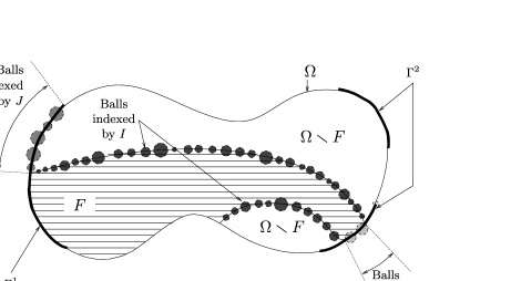
Figure 18: Covering of $(\partial F\cap\Omega)\cup(\partial F\cap\Gamma^{2})\cup(\partial(\Omega\setminus F)\cap\Gamma^{1})$ by balls.

We consider a subsequence of $(R(\mathcal{E}_{n}))_{n\geq}$ that converges toward $F$, but we still denote it by $(R(\mathcal{E}_{n}))_{n\geq 1})$ for simplicity. If $\operatorname{capacity}(F)=0$, there is nothing to prove. Thus we can suppose that $\operatorname{capacity}(F)>0$. In fact it has been proved in CerfTheret09geoc that under hypotheses (H1) and (H2), $\phi_{\Omega}^{b}>0$ if and only if hypothesis (H3) is fulfilled. Thus it is indeed the case that $\operatorname{capacity}(F)>0$.

Step 1: From $V(\mathcal{E}_{n})$ to $\sum_{i}V(\mathcal{E}_{n}\cap B_{i})$ and from $\operatorname{capacity}(F)$ to$\sum_{i}\alpha_{d-1}r_{i}^{d-1}\times\nu(\vec{v}_{i})$. We consider a fixed realization of the capacities. We use Lemma 1 in CerfTheret09infc to cover $\partial F$ by a set of balls well chosen; see Figure 18:

Lemma 2 ((Lemma 1 in CerfTheret09infc ))

Let $F$ be a subset of $\Omega$ of finite perimeter. For every positive constant $\delta$ and $\eta$, there exists a finite family of closed disjoint balls $(B_{i})_{i\in I\cup J\cup K}$ where $B_{i}=(B(x_{i},r_{i}),\vec{v}_{i})$ such that (the vector $\vec{v}_{i}$ defines $B_{i}^{-}$)

$$\forall i\in I,x_{i}\in\partial^{*}F\cap\Omega,\vec{v}_{i}=\vec{v}_{F}(x_{i}),r_{i}\in\,]0,1\bigl{[},B_{i}\subset\Omega,\mathfrak{d}\bigl{(}F\cap B_{i},B_{i}^{-}\bigr{)}\leq\delta\alpha_{d}r_{i}^{d},$$

$$\forall i\in J,x_{i}\in\Gamma^{1}\cap\partial^{*}(\Omega\setminus F),\vec{v}_{i}=\vec{v}_{\Omega}(x_{i}),r_{i}\in\,\bigr{]}0,1\bigl{[},\partial\Omega\cap B_{i}\subset\Gamma^{1},$$

$$\qquad\mathfrak{d}\bigl{(}(\Omega\setminus F)\cap B_{i},B_{i}^{-}\bigr{)}\leq\delta\alpha_{d}r_{i}^{d},$$

$$\forall i\in K,x_{i}\in\Gamma^{2}\cap\partial^{*}F,\vec{v}_{i}=\vec{v}_{F}(x_{i}),r_{i}\in\,\bigr{]}0,1[,\partial\Omega\cap B_{i}\subset\Gamma^{2},$$

$$\qquad\mathfrak{d}\bigl{(}F\cap B_{i},B_{i}^{-}\bigr{)}\leq\delta\alpha_{d}r_{i}^{d},$$

and finally

$$\biggl{|}\operatorname{capacity}(F)-\sum_{i\in I\cup J\cup K}\alpha_{d-1}r_{i}^{d-1}\nu(\vec{v}_{i})\biggr{|}\leq\eta.$$

We do not give the proof of Lemma 2 here. It relies on the Vitali covering theorem for $\mathcal{H}^{d-1}$ and the Besicovitch differentiation theorem in $\mathbb{R}^{d}$.

Remark 21.

In fact, Lemma 1 in CerfTheret09infc states the condition $\mathfrak{d}(B_{i}\cap\Omega,B_{i}^{-})\leq\delta$ instead of $\mathfrak{d}(B_{i}\cap(\Omega\setminus F),B_{i}^{-})\leq\delta$ for $i\in J$. Both statements are true, since we can apply the same techniques to $\Omega$ or $\Omega\setminus F$. However, Lemma 1 in CerfTheret09infc should have been written as Lemma 2 here since the property actually used in Section 5.2 of CerfTheret09infc is in fact $\mathfrak{d}(B_{i}\cap(\Omega\setminus F),B_{i}^{-})\leq\delta$; there is a small mistake in this section on page 653.

We need to move these balls a little bit to obtain balls whose centers have rational coordinates and with $\vec{v}_{i}$ a rational direction. Let $0<\eta,\delta<1$, and let $(B_{i})_{i\in I\cup J\cup K}$ be the family of balls associated to $(\eta/2,\delta/2)$. The function $\nu$ is continuous on $\SS^{d-1}$. Thus there exists $\theta_{0}>0$ such that for all vectors $\vec{v},\vec{w}\in\SS^{d-1}$,

$$\vec{v}\cdot\vec{w}\geq\cos\theta_{0}\quad\Longrightarrow\quad\bigl{|}\nu(\vec{v})-\nu(\vec{w})\bigr{|}\leq\frac{\eta\nu_{\min}}{4\operatorname{capacity}(F)},$$

where $\nu_{\min}=\inf_{\SS^{d-1}}\nu>0$. If for all $i\in I\cup J\cup K$, $\vec{v}_{i}\cdot\vec{v}_{i}^{\prime}\geq\cos\theta_{0}$, we get

$$\biggl{|}\sum_{i\in I\cup J\cup K}\alpha_{d-1}r_{i}^{d-1}\nu(\vec{v}_{i})-\sum_{i\in I\cup J\cup K}\alpha_{d-1}r_{i}^{d-1}\nu\bigl{(}\vec{v}_{i}^{\prime}\bigr{)}\biggr{|}$$

$$\qquad\leq\frac{\eta\nu_{\min}}{4\operatorname{capacity}(F)}\sum_{i\in I\cup J\cup K}\alpha_{d-1}r_{i}^{d-1}$$

$$\qquad\leq\frac{\eta\nu_{\min}}{4\operatorname{capacity}(F)}\frac{2\operatorname{capacity}(F)}{\nu_{\min}}$$

$$\qquad\leq\frac{\eta}{2}.$$

Moreover, for all $x,x^{\prime},r,\vec{v},\vec{v}^{\prime}$ with $\vec{v}\cdot\vec{v}^{\prime}=\cos\theta$ (see Figure 19), we have

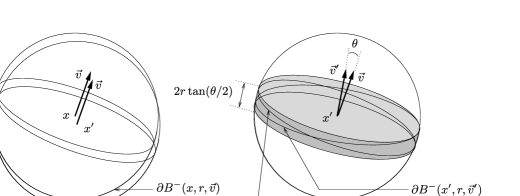
Figure 19: Comparison between $B^{-}(x,r,\vec{v})$ and $B^{-}(x^{\prime},r,\vec{v}^{\prime})$.

$$\mathcal{L}^{d}\bigl{(}B^{-}(x,r,\vec{v})\triangle B^{-}\bigl{(}x^{\prime},r,\vec{v}^{\prime}\bigr{)}\bigr{)}$$

$$\qquad\leq\mathcal{L}^{d}\bigl{(}B^{-}(x,r,\vec{v})\triangle B^{-}\bigl{(}x^{\prime},r,\vec{v}\bigr{)}\bigr{)}+\mathcal{L}^{d}\bigl{(}B^{-}\bigl{(}x^{\prime},r,\vec{v}\bigr{)}\triangle B^{-}\bigl{(}x^{\prime},r,\vec{v}^{\prime}\bigr{)}\bigr{)}$$

$$\qquad\leq\mathcal{L}^{d}\bigl{(}\mathcal{V}_{2}\bigl{(}\partial B^{-}(x,r,\vec{v}),\bigl{\|}x-x^{\prime}\bigr{\|}\bigr{)}\bigr{)}$$

$$\qquad\quad{}+\mathcal{L}^{d}\bigl{(}\operatorname{cyl}\bigl{(}\operatorname{disc}\bigl{(}x^{\prime},r,\bigl{(}\vec{v}+\vec{v}^{\prime}\bigr{)}/2\bigr{)},r\tan(\theta/2)\bigr{)}\bigr{)}$$

$$\qquad\leq\mathcal{L}^{d}\bigl{(}\mathcal{V}_{2}\bigl{(}\partial B^{-}(0,r,\vec{v}),\bigl{\|}x-x^{\prime}\bigr{\|}\bigr{)}\bigr{)}+\alpha_{d-1}r^{d-1}\times 2r\tan(\theta/2)$$

$$\qquad\leq\frac{\delta}{2}\alpha_{d}r^{d},$$

where the last inequality is valid as soon as

$$\tan(\theta/2)\leq\frac{\delta\alpha_{d}}{8\alpha_{d-1}}$$

and

$$\mathcal{L}^{d}\bigl{(}\mathcal{V}_{2}\bigl{(}\partial B^{-}(0,r,\vec{v}),\bigl{\|}x-x^{\prime}\bigr{\|}\bigr{)}\bigr{)}\leq\frac{\delta}{4}\alpha_{d}r^{d}.$$ (82)

We know that $\partial B^{-}(0,r,\vec{v})$ is $(d-1)$-rectifiable. Thus its $(d-1)$ dimensional Minkowski content exists and

$$\lim_{R\rightarrow 0}\frac{\mathcal{L}^{d}(\mathcal{V}_{2}(\partial B^{-}(0,r,\vec{v}),R))}{2R}=\mathcal{H}^{d-1}\bigl{(}\partial B^{-}(0,r,\vec{v})\bigr{)}=Kr^{d-1}$$

for a constant $K$ depending only on the dimension. Thus for $x^{\prime}$ close enough to $x$,

$$\mathcal{L}^{d}\bigl{(}\mathcal{V}_{2}\bigl{(}\partial B^{-}(0,r,\vec{v}),\bigl{\|}x-x^{\prime}\bigr{\|}\bigr{)}\bigr{)}\leq 4\bigl{\|}x-x^{\prime}\bigr{\|}Kr^{d-1},$$

and we obtain (82) for $\|x^{\prime}-x\|$ small enough (how small depending on $d$, $r$ and $\delta$). Thus there exists $\theta_{1}>0$ such that if $\vec{v}_{i}\cdot\vec{v}_{i}^{\prime}\geq\cos\theta_{1}$ for all $i\in I\cup J\cup K$, and if $x_{i}^{\prime}$ is close enough to $x_{i}$, we have

$$\mathcal{L}^{d}\bigl{(}B^{-}(x_{i},r_{i},\vec{v}_{i})\triangle B^{-}\bigl{(}x^{\prime}_{i},r_{i},\vec{v}_{i}^{\prime}\bigr{)}\bigr{)}\leq\frac{\delta}{2}\alpha_{d}r_{i}^{d}.$$

Since $\Omega$ is open and $\Gamma^{1}$ and $\Gamma^{2}$ are open in $\Gamma$, we can choose for all $i\in I\cup J\cup K$ a unit vector $\vec{v}_{i}^{\prime}$ that defines a rational direction, that is, such that $\lambda_{i}\vec{v}_{i}^{\prime}$ has rational coordinates for a positive real number $\lambda_{i}$, and a point $x_{i}^{\prime}$ that has rational coordinates, such that

$$\forall i\in I,r_{i}\in\,]0,1[,B\bigl{(}x^{\prime}_{i},r_{i}\bigr{)}\subset\Omega,\mathfrak{d}\bigl{(}F\cap B\bigl{(}x_{i}^{\prime},r_{i}\bigr{)},B^{-}\bigl{(}x_{i}^{\prime},r_{i},\vec{v}_{i}^{\prime}\bigr{)}\bigr{)}\leq\delta\alpha_{d}r_{i}^{d},$$

$$\forall i\in J,r_{i}\in\,]0,1[,\partial\Omega\cap B\bigl{(}x_{i}^{\prime},r_{i}\bigr{)}\subset\Gamma^{1},\mathfrak{d}\bigl{(}(\Omega\setminus F)\cap B\bigl{(}x_{i}^{\prime},r_{i}\bigr{)},$$

$$\hskip 193.0pt\qquad B^{-}\bigl{(}x_{i}^{\prime},r_{i},\vec{v}_{i}^{\prime}\bigr{)}\bigr{)}\leq\delta\alpha_{d}r_{i}^{d},$$

$$\forall i\in K,r_{i}\in\,]0,1[,\partial\Omega\cap B\bigl{(}x_{i}^{\prime},r_{i}\bigr{)}\subset\Gamma^{2},\mathfrak{d}\bigl{(}F\cap B\bigl{(}x_{i}^{\prime},r_{i}\bigr{)},B^{-}\bigl{(}x_{i}^{\prime},r_{i},\vec{v}_{i}^{\prime}\bigr{)}\bigr{)}\leq\delta\alpha_{d}r_{i}^{d}.$$

For simplicity of notation, we skip the prime and still denote this new family of balls associated to $(\eta,\delta)$ by $(B_{i},i\in I\cup J\cup K)=(B(x_{i},r_{i}),\vec{v}_{i},i\in I\cup J\cup K)$.

Remark 22.

If $\mathfrak{d}(F\cap B(x,r),B^{-}(x,r,\vec{v}))$ is small, $F$ “looks like”$B^{-}(x,r,\vec{v})$ inside the ball $B(x,r)$. This means that the volume of $(F\cap B(x,r))\times\triangle B^{-}(x,r,\vec{v})$ is small; however $F$ (resp., $F^{c}$) might have some thin strands (of small volume, but that can be long) that go deeply into $B^{+}(x,r,\vec{v})$ [resp., $B^{-}(x,r,\vec{v})$]; see Figure 20. If $d\geq 3$, this is not in contradiction with the hypothesis that the capacity of $\partial F$ inside $B(x,r,\vec{v})$ is close to $\alpha_{d-1}r^{d-1}\nu(\vec{v})$.

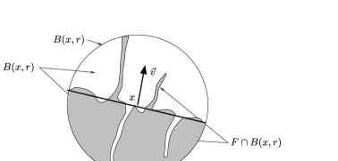
Figure 20: The sets $F\cap B(x,r)$ and $B^{-}(x,r,\vec{v})$.

Let $0<s<1$. We will prove that

$$\liminf_{n\rightarrow\infty}\frac{V(\mathcal{E}_{n})}{n^{d-1}}\geq\operatorname{capacity}(F)(1-2s).$$

We choose

$$\eta=s\operatorname{capacity}(F).$$

We do not fix $\delta$ for the moment, and we consider the family of balls $(B_{i})_{i\in I\cup J\cup K}$ associated to $F$ by Lemma 2 (it depends on $\delta$) via the transformation we did (thus $x_{i}$ and $\vec{v}_{i}$ are rational for all $i$). By construction, we get

$$\biggl{|}\operatorname{capacity}(F)-\sum_{i\in I\cup J\cup K}\alpha_{d-1}r_{i}^{d-1}\nu(\vec{v}_{i})\biggr{|}\leq s\operatorname{capacity}(F).$$ (83)

Since the capacities are nonnegative we have

$$V(\mathcal{E}_{n})=\sum_{e\in\mathcal{E}_{n}}t(e)\geq\sum_{i\in I\cup J\cup K}V(\mathcal{E}_{n}\cap B_{i}),$$ (84)

where $\mathcal{E}_{n}\cap B_{i}=\{e\in\mathcal{E}_{n}|e\subset B_{i}\}$.

Step 2: From $V(\mathcal{E}_{n}\cap B_{i})$ to $\alpha_{d-1}r_{i}^{d-1}\nu(\vec{v}_{i})$.

We define

$$\varepsilon=\varepsilon(\delta)=\delta\min_{i\in I\cup J\cup K}\alpha_{d}r_{i}^{d}.$$

Since $(R(\mathcal{E}_{n}))_{n\geq 1}$ converges toward $F$, this implies that

$$\exists n_{0}\ \forall n\geq n_{0}\qquad\mathfrak{d}\bigl{(}R(\mathcal{E}_{n}),F\bigr{)}\leq\varepsilon.$$ (85)

Let $(B(x,r),\vec{v})=(B_{i}(x_{i},r_{i}),\vec{v}_{i})$ for any $i\in I\cup J\cup K$. Roughly speaking, we control the distance between $R(\mathcal{E}_{n})$ and $F$ by (85), and the distance between $F\cap B$ and $B^{-}$ by construction of the balls. Thus we obtain a control on $\mathfrak{d}(R(\mathcal{E}_{n})\cap B,B^{-})$, and since $R(\mathcal{E}_{n})=r(\mathcal{E}_{n})+[-1,1]^{d}/(2n)$ [thus $r(\mathcal{E}_{n})=R(\mathcal{E}_{n})\cap\mathbb{Z}^{d}_{n}$], this gives us a control on the $\operatorname{card}(r(\mathcal{E}_{n}\cap B)\triangle(B^{-}\cap\mathbb{Z}^{d}_{n}))$.

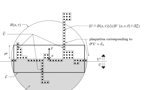
Figure 21: The sets $U$ and $\widetilde{U}$.

More precisely, it is proved in Section 5 of CerfTheret09infc that there exists a set of vertices $U\subset\mathbb{Z}^{d}_{n}$ that satisfies

$$\operatorname{card}\bigl{(}\bigl{(}U\cap B(x,r)\bigr{)}\triangle\bigl{(}B^{-}(x,r,\vec{v})\cap\mathbb{Z}^{d}_{n}\bigr{)}\bigr{)}\leq 4\delta\alpha_{d}r_{i}^{d}n^{d}$$ (86)

and

$$\bigl{(}\partial^{e}U\bigr{)}\cap B=\mathcal{E}_{n}\cap B,$$ (87)

where we generalize the notation we have adopted for $\mathcal{E}_{n}\cap B_{i}$; see Figure 21. This statement is a bit more elaborated than expected because of the slight difference between balls indexed in $I,J$ and $K$: we can choose $U=r(\mathcal{E}_{n})$ if $B=B_{i}$ for $i\in I\cup K$ and $U=\Omega_{n}\setminus r(\mathcal{E}_{n})$ if $B=B_{i}$ for $i\in J$. We define the cylinder $\mathcal{C}\subset B(x,r)$ by

$$\mathcal{C}=\operatorname{cyl}\bigl{(}\operatorname{disc}\bigl{(}x,r^{\prime},\vec{v}\bigr{)},\rho r\bigr{)},$$

where $\rho$ is a positive constant we have to choose and $r^{\prime}=r\cos(\arcsin\rho)$. It is proved in Section 6 of CerfTheret09infc that there exists a set of edges $\widetilde{U}$ (denoted by $X^{+}\cup X^{-}$ in that paper) included in $B$ such that $(B\cap\partial^{e}U)\cup\widetilde{U}$ contains a cutset from the top to the bottom of $\mathcal{C}$ in the direction $\vec{v}$ (see Figure 21) and

$$\operatorname{card}(\widetilde{U})\leq Cr^{d-1}\delta\rho^{-1}n^{d-1},$$

where $C=10d\alpha_{d}$ is a constant that depends only on the dimension. We denote by $\phi_{\mathcal{C}}$ the maximal flow from the top to the bottom of $\mathcal{C}$, that is, $\phi_{\mathcal{C}}=\phi(T(\operatorname{disc}(x,r^{\prime},\vec{v}),\rho r),B(\operatorname{disc}(x,r^{\prime},\vec{v}),\rho r),\mathcal{C})$. Thus, by the maximality of $\phi_{\mathcal{C}}$ and thanks to equation (87),

$$\phi_{\mathcal{C}} \leq V\bigl{(}\partial^{e}U\cap B\bigr{)}+MCr^{d-1}\delta\rho^{-1}n^{d-1}$$

$$= V(\mathcal{E}_{n}\cap B)+MCr^{d-1}\delta\rho^{-1}n^{d-1}.$$

To complete the proof, it remains to compare $\phi_{\mathcal{C}}$ with $\alpha_{d-1}r^{d-1}\nu(\vec{v})n^{d-1}$. This is done in Section 6 of CerfTheret09infc by almost covering $\operatorname{disc}(x,r^{\prime},\vec{v})$ with a finite family of disjoint closed hyperrectangles $(a_{i})_{i\in\mathcal{I}}$ satisfying, for a constant $c=c(d)$ and chosen $\kappa>0$ as small as we want,

$$\sum_{i\in\mathcal{I}}\mathcal{H}^{d-1}(a_{i})>\alpha_{d-1}r^{\prime d-1}-\kappa\quad\mbox{and}\quad\sum_{i\in\mathcal{I}}\mathcal{H}^{d-2}(\partial a_{i})<cr^{\prime d-2}.$$

Thus the cylinders $(\operatorname{cyl}(a_{i},\rho r))_{i\in\mathcal{I}}$ almost fill $\mathcal{C}$. Since $x$ has rational coordinates and $\vec{v}$ is a rational unit vector (i.e., $\lambda\vec{v}$ has rational coordinates for a positive real number $\lambda$), we can choose the hyperrectangles $(a_{i},i\in\mathcal{I})$ with rational vertices. Indeed, we explained in Section 4.5 that there exist vectors $\vec{u}_{i}$, $i=2,\ldots,d$ that have integer coordinates and such that $(\vec{v},\vec{u}_{2},\ldots,\vec{u}_{d})$ is an orthogonal basis of $\mathbb{R}^{d}$. Then any hyperrectangle of the form $x+\sum_{i=2}^{d}\lambda_{i}\vec{u}_{i}+\prod_{i=2}^{d}[0,\mu_{i}\vec{u}_{i}]$ with rational $\lambda_{i},\mu_{i}$ has rational vertices. We can choose the hyperrectangles $(a_{i},i\in\mathcal{I})$ of this type; see Figure 22.

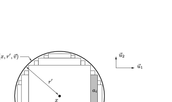
Figure 22: The sets $\operatorname{disc}(x,r^{\prime},\vec{v})$ and $(a_{i},i\in\mathcal{I})$.

Let $h\in[\rho r,2\rho r]\cap\mathbb{Q}$. The cylinders $\operatorname{cyl}(a_{i},h)$, $i\in\mathcal{I}$, have rational vertices. If $\mathcal{F}_{n}$ is a cutset from the top to the bottom of $\mathcal{C}$, then $\mathcal{F}_{n}\cap\operatorname{cyl}(a_{i},\rho r)$ is a cutset from the top to the bottom of $\operatorname{cyl}(a_{i},h)$, and if we add to $\mathcal{F}_{n}\cap\operatorname{cyl}(a_{i},\rho r)$ some edges along the vertical sides of $\operatorname{cyl}(a_{i},h)$, we obtain a cutset in $\operatorname{cyl}(a_{i},h)$ between the lower half part and the upper half part of its boundary. More formally, if we define

$$\mathcal{P}_{i}(n)=\operatorname{cyl}\bigl{(}\mathcal{V}_{2}(\partial a_{i},2d/n)\cap\operatorname{hyp}(a_{i}),h\bigr{)},$$

and if we denote by $P_{i}(n)$ the set of the edges included in $\mathcal{P}_{i}(n)$, we get

$$\sum_{i\in\mathcal{I}}\tau\bigl{(}\operatorname{cyl}(a_{i},\rho r),\vec{v}\bigr{)}\leq\phi_{\mathcal{C}}+V\biggl{(}\bigcup_{i\in\mathcal{I}}P_{i}(n)\biggr{)}$$

for a complete proof, we refer to Section 6 of CerfTheret09infc . Moreover,

$$\operatorname{card}\biggl{(}\bigcup_{i\in\mathcal{I}}P_{i}(n)\biggr{)}\leq c^{\prime}\rho r^{d-1}n^{d-1},$$

where $c^{\prime}$ is a constant depending on the dimension, thus

$$\phi_{\mathcal{C}}\geq\sum_{i\in\mathcal{I}}\tau\bigl{(}\operatorname{cyl}(a_{i},\rho r),\vec{v}\bigr{)}-Mc^{\prime}\rho r^{d-1}n^{d-1}.$$ (89)

Combining inequalities (5.3) and (89), we get

$$V(\mathcal{E}_{n}\cap B)\geq\sum_{i\in\mathcal{I}}\tau\bigl{(}\operatorname{cyl}(a_{i},h),\vec{v}\bigr{)}-Mr^{d-1}c^{\prime\prime}\bigl{(}\rho+\delta\rho^{-1}\bigr{)}n^{d-1}$$ (90)

for a constant $c^{\prime\prime}$ depending on the dimension. Theorem 2.2 states that for every cylinder $\operatorname{cyl}(A,h)$ with $A$ a nondegenerate hyperrectangle normal to $\vec{v}$ and $h>0$, we have

$$\lim_{n\rightarrow\infty}\frac{\tau_{n}(\operatorname{cyl}(A,h),\vec{v})}{n^{d-1}\mathcal{H}^{d-1}(A)}=\nu(\vec{v})\qquad\mbox{a.s.}$$

Thus these convergences hold a.s. simultaneously for all the rational cylinders, that is, cylinders with rational vertices [like the cylinders $(\operatorname{cyl}(a_{i},h),\break i\in\mathcal{I})$]. We consider only realizations of the capacities on which these convergences occur. Combined with inequality (90), this implies that

$$\liminf_{n\rightarrow\infty}\frac{V(\mathcal{E}_{n}\cap B)}{n^{d-1}}$$

$$\qquad\geq\biggl{(}\sum_{i\in\mathcal{I}}\mathcal{H}^{d-1}(a_{i})\biggr{)}\nu(\vec{v})-Mr^{d-1}c^{\prime\prime}\bigl{(}\rho+\delta\rho^{-1}\bigr{)}$$

$$\qquad\geq\bigl{(}\alpha_{d-1}r^{\prime d-1}-\kappa\bigr{)}\nu(\vec{v})-Mr^{d-1}c^{\prime\prime}\bigl{(}\rho+\delta\rho^{-1}\bigr{)}$$

$$\qquad\geq\alpha_{d-1}r^{d-1}\nu(\vec{v})-\alpha_{d-1}\bigl{(}r^{d-1}-r^{\prime d-1}\bigr{)}\nu(\vec{v})-\kappa\nu(\vec{v})$$

$$\qquad\quad{}-Mr^{d-1}c^{\prime\prime}\bigl{(}\rho+\delta\rho^{-1}\bigr{)}.$$

We choose $\rho=\sqrt{\delta}$ and $\kappa=\alpha_{d-1}(r^{d-1}-r^{\prime d-1})$. We define

$$\nu_{\min}=\min_{\vec{v}\in\SS^{d-1}}\nu(\vec{v})\quad\mbox{and}\quad\nu_{\max}=\max_{\vec{v}\in\SS^{d-1}}\nu(\vec{v}).$$

Under hypothesis (H3), we have $0<\nu_{\min}\leq\nu_{\max}<+\infty$. Since $r^{\prime}=\break r\cos(\arcsin\rho)$, we get

$$\liminf_{n\rightarrow\infty}\frac{V(\mathcal{E}_{n}\cap B)}{n^{d-1}}$$

$$\qquad\geq\alpha_{d-1}r^{d-1}\nu(\vec{v})$$ (91)

$$\qquad\quad{}-2\alpha_{d-1}r^{d-1}\nu_{\max}\bigl{[}1-\bigl{(}\cos(\arcsin\sqrt{\delta})\bigr{)}^{d-1}\bigr{]}-2Mc^{\prime\prime}\sqrt{\delta}r^{d-1}.$$

Equations (83), (84) and (5.3), and the fact that $\sum_{i}\alpha_{d-1}r_{i}^{d-1}\leq\break\operatorname{capacity}(F)(1+s)\nu_{\min}^{-1}$, give

$$\liminf_{n\rightarrow\infty}\frac{V(\mathcal{E}_{n})}{n^{d-1}}\geq\operatorname{capacity}(F)(1-s-w),$$ (92)

where

$$w=4\frac{\nu_{\max}}{\nu_{\min}}\bigl{[}1-\bigl{(}\cos(\arcsin\sqrt{\delta})\bigr{)}^{d-1}\bigr{]}+\frac{4Mc^{\prime\prime}}{\alpha_{d-1}}\sqrt{\delta}.$$ (93)

For $\delta$ small enough, $w\leq s$, and we get

$$\liminf_{n\rightarrow\infty}\frac{V(\mathcal{E}_{n})}{n^{d-1}}\geq\operatorname{capacity}(F)(1-2s).$$

This completes the proof of Proposition 5.3.

6 Continuous max-flow min-cut theorem

6.1 Comparison between continuous streams and cutsets

Proof of Lemma 1 Let $\vec{\sigma}$ be an admissible continuous stream, that is:

• $\vec{\sigma}\in L^{\infty}\bigl{(}\mathbb{R}^{d}\rightarrow\mathbb{R}^{d},\mathcal{L}^{d}\bigr{)}\mbox{ and }\vec{\sigma}=0\ \mathcal{L}^{d}\mbox{-a.e. on }\Omega^{c},$

• $\operatorname{div}\vec{\sigma}=0\ \mathcal{L}^{d}\mbox{-a.e. on }\Omega,$

• $\vec{\sigma}\cdot\vec{v}\leq\nu(\vec{v})\mbox{ for all }\vec{v}\in\SS^{d-1}\ \mathcal{L}^{d}\mbox{-a.e. on }\Omega,$

• $\vec{\sigma}\cdot\vec{v}_{\Omega}\leq 0\ \mathcal{H}^{d-1}\mbox{-a.e. on }\Gamma^{1}\mbox{ and }\vec{\sigma}\cdot\vec{v}_{\Omega}=0\ \mathcal{H}^{d-1}\mbox{-a.e. on }\Gamma\setminus\bigl{(}\Gamma^{1}\cup\Gamma^{2}\bigr{)}.$

As in Remark 13 in Section 4.4, we obtain

$$\forall u\in\mathcal{C}_{c}^{\infty}\bigl{(}\mathbb{R}^{d},\mathbb{R}\bigr{)}$$

$$\qquad\int_{\mathbb{R}^{d}}u\operatorname{div}\vec{\sigma}\,d\mathcal{L}^{d}=-\int_{\mathbb{R}^{d}}\vec{\sigma}\cdot\vec{\nabla}u\,d\mathcal{L}^{d}\qquad\mbox{by definition of }\operatorname{div}\vec{\sigma}$$

$$\hskip 70.0pt\qquad=-\int_{\Gamma}(\vec{\sigma}\cdot\vec{v}_{\Omega})u\,d\mathcal{H}^{d-1}\qquad\mbox{ by definition of }\vec{\sigma}\cdot\vec{v}_{\Omega},$$

where for the last equality we have used the characterization of $\vec{\sigma}\cdot\vec{v}_{\Omega}$ given in equation (50). Thus $\operatorname{div}\vec{\sigma}\,d\mathcal{L}^{d}$ is not only a distribution but also a measure, and this measure is equal to $(\vec{\sigma}\cdot\vec{v}_{\Omega})\,d\mathcal{H}^{d-1}|_{\Gamma}$. Therefore we can apply to $\vec{\sigma}$ the techniques used in Section 4.6. We consider a polyhedral set $P\subset\mathbb{R}^{d}$ such that

$$\overline{\Gamma}^{1}\subset\stackrel{{\scriptstyle\circ}}{{P}},\qquad\overline{\Gamma}^{2}\subset\,\stackrel{{\scriptstyle\circ}}{{\wideparen{\mathbb{R}^{d}\setminus P}}}\quad\mbox{and}\quad\partial P\mbox{ is transversal to }\Gamma.$$

For any positive $\eta$, there exists $h_{0}>0$ such that for all $0<h<h_{0}$ we obtain inequality (4.6),

$$\Biggl{|}\operatorname{flow}^{\mathrm{cont}}(\vec{\sigma})-\frac{1}{2h}\sum_{i=1}^{\mathcal{N}}\int_{\operatorname{cyl}(A_{i},h)}\vec{\sigma}\cdot\vec{v}_{i}\,d\mathcal{L}^{d}\Biggr{|}\leq C\eta\|\vec{\sigma}\|_{\infty}.$$

We have $\vec{\sigma}\cdot\vec{v}\leq\nu(\vec{v})$ and $-\vec{\sigma}\cdot\vec{v}\leq\nu(-\vec{v})=\nu(\vec{v})$ $\mathcal{L}^{d}$-a.e., thus $|\vec{\sigma}\cdot\vec{v}|\leq\nu(\vec{v})$ $\mathcal{L}^{d}$-a.e. We obtain

$$\operatorname{flow}^{\mathrm{cont}}(\vec{\sigma}) \leq \frac{1}{2h}\sum_{i=1}^{\mathcal{N}}\int_{\operatorname{cyl}(A_{i},h)}\vec{\sigma}\cdot\vec{v}_{i}\,d\mathcal{L}^{d}+C\eta\|\vec{\sigma}\|_{\infty}$$

$$\leq \frac{1}{2h}\sum_{i=1}^{\mathcal{N}}\nu(\vec{v}_{i})\mathcal{L}^{d}\bigl{(}\operatorname{cyl}(A_{i},h)\bigr{)}+C\eta\|\vec{\sigma}\|_{\infty}$$

$$\leq \frac{1}{2h}\sum_{i=1}^{\mathcal{N}}\nu(\vec{v}_{i})2h\mathcal{H}^{d-1}(A_{i})+C\eta\|\vec{\sigma}\|_{\infty}$$

$$\leq \sum_{i=1}^{\mathcal{N}}\nu(\vec{v}_{i})\mathcal{H}^{d-1}(A_{i})+C\eta\|\vec{\sigma}\|_{\infty}$$

$$\leq \int_{\partial P\cap\Omega^{\prime}}\nu(\vec{v}_{P})\,d\mathcal{H}^{d-1}+C\eta\|\vec{\sigma}\|_{\infty}$$

$$\leq \operatorname{capacity}(P\cap\Omega)+\nu_{\max}\mathcal{H}^{d-1}\bigl{(}\partial P\cap\bigl{(}\Omega^{\prime}\setminus\Omega\bigr{)}\bigr{)}+C\eta\|\vec{\sigma}\|_{\infty}$$

$$\leq \operatorname{capacity}(P\cap\Omega)+\nu_{\max}\widehat{\eta}+C\eta\|\vec{\sigma}\|_{\infty},$$

where we have used inequality (69) to control $\mathcal{H}^{d-1}(\partial P\cap(\Omega^{\prime}\setminus\Omega))$, and where $\nu_{\max}=\max_{\SS^{d-1}}\nu$. Since $\eta$ and $\widehat{\eta}$ are arbitrarily small, for all $P\subset\mathbb{R}^{d}$ such that $\overline{\Gamma}^{1}\subset\stackrel{{\scriptstyle\circ}}{{P}}$, $\overline{\Gamma}^{2}\subset\stackrel{{\scriptstyle\circ}}{{\wideparen{\mathbb{R}^{d}\setminus P}}}$ and $\partial P$ is transversal to $\Gamma$, we obtain

$$\operatorname{flow}^{\mathrm{cont}}(\vec{\sigma})\leq\operatorname{capacity}(P\cap\Omega).$$ (94)

The following result has been proved in CerfTheret09geoc :

Theorem 6.1 ((Theorem 11 in CerfTheret09geoc ))

We suppose that hypotheses (H1) are fulfilled, and that the law of the capacities is integrable,

$$\int_{\mathbb{R}^{+}}x\,d\Lambda(x)<+\infty.$$

Let $F$ be a subset of $\Omega$ having finite perimeter in $\Omega$. For any $\varepsilon>0$, there exists a polyhedral set $P$ whose boundary $\partial P$ is transversal to $\Gamma$ and such that

$$\displaystyle\overline{\Gamma}^{1}\subset\stackrel{{\scriptstyle\circ}}{{P}},\qquad\overline{\Gamma}^{2}\subset\stackrel{{\scriptstyle\circ}}{{\wideparen{\mathbb{R}^{d}\setminus P}}},\qquad\mathcal{L}^{d}\bigl{(}F\triangle(P\cap\Omega)\bigr{)}<\varepsilon,$$

$$\displaystyle\int_{\partial^{*}P\cap\Omega}\nu\bigl{(}\vec{v}_{P}(x)\bigr{)}\,d\mathcal{H}^{d-1}(x)=\operatorname{capacity}(P\cap\Omega)\leq\operatorname{capacity}(F)+\varepsilon.$$

Combining inequality (94) and Theorem 6.1, we obtain that for all $F\subset\Omega$ such that $\mathbh{1}_{F}\in\operatorname{BV}(\Omega)$,

$$\operatorname{flow}^{\mathrm{cont}}(\vec{\sigma})\leq\operatorname{capacity}(F),$$

and thus Lemma 1 is proved.

6.2 End of the proofs of Theorems 1.1, 1.2, 1.3 and 1.4

We suppose first that hypothesis (H3) is fulfilled. Let $(\vec{\mu}_{n}^{\max})_{n\geq 1}$ be a sequence of discrete maximal streams and $(\mathcal{E}_{n}^{\min})_{n\geq 1}$ be a sequence of discrete minimal cutsets. From a subsequence of $(\vec{\mu}_{n}^{\max})_{n\geq 1}$ that converges weakly toward a measure $\vec{\mu}=\vec{\sigma}\mathcal{L}^{d}$, we can a.s. extract a sub-subsequence $(\vec{\mu}_{\varphi(n)}^{\max})_{n\geq 1}$ such that $(R(\mathcal{E}_{\varphi(n)}^{\min}))_{n\geq 1}$ converges also for the distance $\mathfrak{d}$ toward a set $F\subset\Omega$ of finite perimeter. Conversely, from a subsequence of $(R(\mathcal{E}_{n}^{\min}))_{n\geq 1}$ that converges for the distance $\mathfrak{d}$ to a set $F\subset\Omega$ of finite perimeter, we can extract a sub-subsequence $(R(\mathcal{E}_{\varphi(n)}^{\min}))_{n\geq 1}$ such that $(\vec{\mu}_{\varphi(n)}^{\max})_{n\geq 1}$ converges weakly toward a measure $\vec{\mu}=\vec{\sigma}\mathcal{L}^{d}$. Combining Propositions 4.7 and 5.3, we obtain that a.s.

$$\operatorname{capacity}(F) \leq \liminf_{n\rightarrow\infty}\frac{V(\mathcal{E}^{\min}_{\varphi(n)})}{\varphi(n)^{d-1}}=\lim_{n\rightarrow\infty}\frac{\phi_{\varphi(n)}}{\varphi(n)^{d-1}}$$

$$= \lim_{n\rightarrow\infty}\operatorname{flow}^{\mathrm{disc}}_{\varphi(n)}\bigl{(}\vec{\mu}_{\varphi(n)}^{\max}\bigr{)}=\operatorname{flow}^{\mathrm{cont}}(\vec{\sigma}).$$

Since Lemma 1 implies that

$$\operatorname{capacity}(F)\geq\phi_{\Omega}^{a}\geq\phi_{\Omega}^{b}\geq\operatorname{flow}^{\mathrm{cont}}(\vec{\sigma}),$$

combining inequality (6.2) and Lemma 1, we obtain that a.s.

$$\operatorname{capacity}(F)=\phi_{\Omega}^{a}=\phi_{\Omega}^{b}=\operatorname{flow}^{\mathrm{cont}}(\vec{\sigma}).$$

If hypothesis (H3) is not fulfilled, then $\nu=0$, $\phi_{\Omega}^{a}=0$, and Lemma 1 implies that $\phi_{\Omega}^{b}=\phi_{\Omega}^{a}=0$, thus all the admissible continuous streams in $\Sigma^{b}$ are null and all the admissible continuous cutsets have null capacity and are in $\Sigma^{a}$. This completes the proofs of Theorems 1.1, 1.2 and 1.3.

Let us prove Theorem 1.4. We notice that if a subsequence of $(\phi_{n}/n^{d-1})_{n\geq 1}$ converges toward a real variable $\phi$, then we can extract a sub-subsequence $(\phi_{\varphi(n)}/\varphi(n)^{d-1})_{n\geq 1}$ along which the maximal flows converge toward $\phi$ and the maximal streams $(\vec{\mu}_{\varphi(n)}^{\max})_{n\geq 1}$ converge toward a continuous stream $\vec{\sigma}$. Then by Proposition 4.7 and Theorem 1.1 we know that a.s.

$$\phi=\lim_{n\rightarrow\infty}\frac{\phi_{\varphi(n)}}{\varphi(n)^{d-1}}=\operatorname{flow}^{\mathrm{cont}}(\vec{\sigma})=\phi_{\Omega}^{b}.$$ (96)

We claim that $(\phi_{n}/n^{d-1})_{n\geq 1}$ takes its values in a deterministic compact of $\mathbb{R}^{d}$—this, together with equation (96), completes the proof of Theorem 1.4. Indeed, let $P$ be a polyhedral set of $\mathbb{R}^{d}$ such that

$$\overline{\Gamma}^{1}\subset\stackrel{{\scriptstyle\circ}}{{P}}\quad\mbox{and}\quad\overline{\Gamma}^{2}\subset\stackrel{{\scriptstyle\circ}}{{\wideparen{\mathbb{R}^{d}\setminus P}}}.$$

We define

$$\mathcal{F}_{n}=\{e\in\Pi_{n}|e\cap\partial P\neq\varnothing\}.$$

At least for $n$ large enough, $\mathcal{F}_{n}$ separates $\Gamma^{1}_{n}$ from $\Gamma^{2}_{n}$ in $\Omega_{n}$, thus

$$\frac{\phi_{n}}{n^{d-1}}\leq V(\mathcal{F}_{n})\leq M\frac{\operatorname{card}(\mathcal{F}_{n})}{n^{d-1}},$$

and since the $(d-1)$ dimensional Minkowski content of $\partial P\cap\Omega$ exists and is equal to $\mathcal{H}^{d-1}(\partial P\cap\Omega)$, for $n$ large enough we get

$$\operatorname{card}(\mathcal{F}_{n}) \leq 2d\operatorname{card}\bigl{(}\mathcal{V}_{\infty}(\partial P\cap\Omega,2/n)\cap\mathbb{Z}^{d}_{n}\bigr{)}\leq 2dn^{d}\mathcal{L}^{d}\bigl{(}\mathcal{V}_{\infty}(\partial P\cap\Omega,3/n)\bigr{)}$$

$$\leq n^{d-1}K\mathcal{H}^{d-1}(\partial P\cap\Omega)$$

for a constant $K$ that depends on $d$.

References

- (1) {barticle}[mr] \bauthor\bsnmBlum, \bfnmWolfgang\binitsW. (\byear1990). \btitleA measure-theoretical max-flow-min-cut problem. \bjournalMath. Z. \bvolume205 \bpages451–470. \biddoi=10.1007/BF02571255, issn=0025-5874, mr=1082867 \bptokimsref \endbibitem
- (2) {bbook}[mr] \bauthor\bsnmBogachev, \bfnmV. I.\binitsV. I. (\byear2007). \btitleMeasure Theory. Vol. I, II. \bpublisherSpringer, \blocationBerlin. \biddoi=10.1007/978-3-540-34514-5, mr=2267655 \bptokimsref \endbibitem
- (3) {bbook}[mr] \bauthor\bsnmBollobás, \bfnmBéla\binitsB. (\byear1979). \btitleGraph Theory: An Introductory Course. \bseriesGraduate Texts in Mathematics \bvolume63. \bpublisherSpringer, \blocationNew York. \bidmr=0536131 \bptokimsref \endbibitem
- (4) {bbook}[mr] \bauthor\bsnmCerf, \bfnmR.\binitsR. (\byear2006). \btitleThe Wulff Crystal in Ising and Percolation Models. \bseriesLecture Notes in Math. \bvolume1878. \bpublisherSpringer, \blocationBerlin. \bidmr=2241754 \bptokimsref \endbibitem
- (5) {barticle}[mr] \bauthor\bsnmCerf, \bfnmRaphaël\binitsR. and \bauthor\bsnmPisztora, \bfnmÁgoston\binitsÁ. (\byear2001). \btitlePhase coexistence in Ising, Potts and percolation models. \bjournalAnn. Inst. Henri Poincaré Probab. Stat. \bvolume37 \bpages643–724. \biddoi=10.1016/S0246-0203(01)01083-4, issn=0246-0203, mr=1863274 \bptokimsref \endbibitem
- (6) {barticle}[mr] \bauthor\bsnmCerf, \bfnmRaphaël\binitsR. and \bauthor\bsnmThéret, \bfnmMarie\binitsM. (\byear2011). \btitleLaw of large numbers for the maximal flow through a domain of in first passage percolation. \bjournalTrans. Amer. Math. Soc. \bvolume363 \bpages3665–3702. \biddoi=10.1090/S0002-9947-2011-05341-9, issn=0002-9947, mr=2775823 \bptokimsref \endbibitem
- (7) {barticle}[mr] \bauthor\bsnmCerf, \bfnmRaphaël\binitsR. and \bauthor\bsnmThéret, \bfnmMarie\binitsM. (\byear2011). \btitleLower large deviations for the maximal flow through a domain of in first passage percolation. \bjournalProbab. Theory Related Fields \bvolume150 \bpages635–661. \biddoi=10.1007/s00440-010-0287-6, issn=0178-8051, mr=2824869 \bptokimsref \endbibitem
- (8) {barticle}[mr] \bauthor\bsnmCerf, \bfnmRaphaël\binitsR. and \bauthor\bsnmThéret, \bfnmMarie\binitsM. (\byear2011). \btitleUpper large deviations for the maximal flow through a domain of in first passage percolation. \bjournalAnn. Appl. Probab. \bvolume21 \bpages2075–2108. \biddoi=10.1214/10-AAP732, issn=1050-5164, mr=2895410 \bptokimsref \endbibitem
- (9) {bbook}[mr] \bauthor\bsnmFederer, \bfnmHerbert\binitsH. (\byear1969). \btitleGeometric Measure Theory. \bpublisherSpringer, \blocationNew York. \bidmr=0257325 \bptokimsref \endbibitem
- (10) {bbook}[mr] \bauthor\bsnmGiusti, \bfnmEnrico\binitsE. (\byear1984). \btitleMinimal Surfaces and Functions of Bounded Variation. \bseriesMonographs in Mathematics \bvolume80. \bpublisherBirkhäuser, \blocationBasel. \bidmr=0775682 \bptokimsref \endbibitem
- (11) {bbook}[mr] \bauthor\bsnmGuillemin, \bfnmVictor\binitsV. and \bauthor\bsnmPollack, \bfnmAlan\binitsA. (\byear1974). \btitleDifferential Topology. \bpublisherPrentice-Hall, \blocationEnglewood Cliffs, NJ. \bidmr=0348781 \bptokimsref \endbibitem
- (12) {bincollection}[mr] \bauthor\bsnmKesten, \bfnmHarry\binitsH. (\byear1986). \btitleAspects of first passage percolation. In \bbooktitleÉcole D’été de Probabilités de Saint-Flour, XIV—1984. \bseriesLecture Notes in Math. \bvolume1180 \bpages125–264. \bpublisherSpringer, \blocationBerlin. \biddoi=10.1007/BFb0074919, mr=0876084 \bptokimsref \endbibitem
- (13) {barticle}[mr] \bauthor\bsnmKesten, \bfnmHarry\binitsH. (\byear1987). \btitleSurfaces with minimal random weights and maximal flows: A higher-dimensional version of first-passage percolation. \bjournalIllinois J. Math. \bvolume31 \bpages99–166. \bidissn=0019-2082, mr=0869483 \bptokimsref \endbibitem
- (14) {bbook}[mr] \bauthor\bsnmMattila, \bfnmPertti\binitsP. (\byear1995). \btitleGeometry of Sets and Measures in Euclidean Spaces: Fractals and Rectifiability. \bseriesCambridge Studies in Advanced Mathematics \bvolume44. \bpublisherCambridge Univ. Press, \blocationCambridge. \bidmr=1333890 \bptokimsref \endbibitem
- (15) {barticle}[mr] \bauthor\bsnmNozawa, \bfnmRyōhei\binitsR. (\byear1990). \btitleMax-flow min-cut theorem in an anisotropic network. \bjournalOsaka J. Math. \bvolume27 \bpages805–842. \bidissn=0030-6126, mr=1088184 \bptokimsref \endbibitem
- (16) {barticle}[mr] \bauthor\bsnmRossignol, \bfnmRaphaël\binitsR. and \bauthor\bsnmThéret, \bfnmMarie\binitsM. (\byear2010). \btitleLower large deviations and laws of large numbers for maximal flows through a box in first passage percolation. \bjournalAnn. Inst. Henri Poincaré Probab. Stat. \bvolume46 \bpages1093–1131. \biddoi=10.1214/09-AIHP346, issn=0246-0203, mr=2744888 \bptokimsref \endbibitem
- (17) {bbook}[mr] \bauthor\bsnmRudin, \bfnmWalter\binitsW. (\byear1987). \btitleReal and Complex Analysis, \bedition3rd ed. \bpublisherMcGraw-Hill, \blocationNew York. \bidmr=0924157 \bptokimsref \endbibitem
- (18) {bbook}[mr] \bauthor\bsnmSchwartz, \bfnmL.\binitsL. (\byear1950). \btitleThéorie des Distributions. Tome I. \bpublisherHermann, \blocationParis. \bidmr=0035918 \bptokimsref \endbibitem
- (19) {bbook}[mr] \bauthor\bsnmSchwartz, \bfnmLaurent\binitsL. (\byear1951). \btitleThéorie des Distributions. Tome II. \bpublisherHermann, \blocationParis. \bidmr=0041345 \bptokimsref \endbibitem
- (20) {barticle}[mr] \bauthor\bsnmStrang, \bfnmGilbert\binitsG. (\byear1983). \btitleMaximal flow through a domain. \bjournalMath. Program. \bvolume26 \bpages123–143. \biddoi=10.1007/BF02592050, issn=0025-5610, mr=0700642 \bptokimsref \endbibitem
- (21) {barticle}[mr] \bauthor\bsnmZhang, \bfnmYu\binitsY. (\byear2000). \btitleCritical behavior for maximal flows on the cubic lattice. \bjournalJ. Stat. Phys. \bvolume98 \bpages799–811. \biddoi=10.1023/A:1018631726709, issn=0022-4715, mr=1749233 \bptokimsref \endbibitem
- (22) {bmisc}[auto:STB—2013/10/03—07:39:35] \bauthor\bsnmZhang, \bfnmYu\binitsY. (\byear2007). \bhowpublishedLimit theorems for maximum flows on a lattice. Available at arxiv.org/abs/0710.4589. \bptokimsref \endbibitem