Cyclic homology of Fukaya categories and
the linearized contact homology

Abstract.

Let $M$ be an exact symplectic manifold with contact type boundary such that $c_{1}(M)=0$. In this paper we show that the cyclic cohomology of the Fukaya category of $M$ has the structure of an involutive Lie bialgebra. Inspired by a work of Cieliebak-Latschev we show that there is a Lie bialgebra homomorphism from the linearized contact homology of $M$ to the cyclic cohomology of the Fukaya category. Our study is also motivated by string topology and 2-dimensional topological conformal field theory.

1. Introduction

During the past two decades, great achievements have been obtained in the understanding of the geometry and topology of symplectic manifolds. Among them are the Fukaya category of symplectic manifolds, originated by Fukaya ([16]), and the symplectic field theory (SFT), introduced by Eliashberg-Givental-Hofer ([14]). In this paper, we study the cyclic homology of the Fukaya category of an exact symplectic manifold with contact type boundary and its relations to the linearized contact homology defined in SFT.

The main motivation of our study is Kontsevich and Costello’s work on topological conformal field theories ([29, 30] and [13]), and the work of Cieliebak-Latschev ([12]), which studies the algebraic structures on the linearized contact homology and their relations with string topology. Let us explain in more detail.

1.1.

In [30] Kontsevich associates to an A_∞ algebra with a cyclically invariant inner product a cohomology class on the compactified moduli spaces of marked Riemann surfaces, and from this as well as some analogous examples he first raised his theory of noncommutative symplectic geometries. Such an A_∞ algebra was later called by him a Calabi-Yau A_∞ algebra, and was systematically studied in his work with Soibelman ([31]). In his talk at the Hodge Centennial Conference ([30]) he showed that a Calabi-Yau A_∞ algebra, or more generally, a Calabi-Yau A_∞ algebra “with several objects”, i.e. a Calabi-Yau A_∞ category, is an open topological conformal field theory (TCFT), and its Hochschild cohomology is in fact a closed topological conformal field theory. As a particular example, he conjectured that the Fukaya category of a symplectic manifold is a Calabi-Yau category. Similar restults have been obtained by Costello in [13]. We refer the reader to Getzler [22, 23] and Costello [13] for more details and interesting results about TCFT’s. Inspired by [30] and string topology ([9]), the first author showed that the cyclic cohomology of a Calabi-Yau A_∞ category endows the structure of an involutive Lie bialgebra ([11]).

While the existence of the cyclically invariant inner product on the Fukaya category is still under verification (for some partial results see [18]), the work of Kontsevich and Costello remains a guiding philosophy for our study. Our first theorem in the following says that the Lie bialgebra exists on the cyclic cohomology of the Fukaya category (no non-degenerate pairing is assumed):

Theorem A (Theorem 18).

Let $M$ be an exact symplectic manifold with contact type boundary such that $c_{1}(M)=0$. Then the cyclic cohomology of Fukaya category $\mathcal{F}uk(M)$ of $M$ has the structure of an involutive Lie bialgebra.

The key point in the above theorem is that, in the construction of the Fukaya category, counting the pseudo-holomorphic disks is a priori cyclically invariant.

Let $M$ be as in Theorem A. Denote its boundary by $W$. The symplectic field theory of Eliashberg-Givental-Hofer relates the geometry of closed Reeb orbits on $W$ with the geometry of pseudo-holomorphic curves on the symplectic completion $\widehat{M}$ of $M$. In fact, pseudo-holomorphic curves in $\widehat{M}$ asymptotic to closed Reeb orbits share a lot of properties of a closed TCFT; for more details, see [14]. Among all the interesting properties of SFT, Cieliebak-Latschev ([12, Theorem A]) proved that the linearized contact homology of $M$, denoted by $\mathrm{CH}^{\mathrm{lin}}_{*}(M)$, which basically arises from counting the pseudo-holomorphic cyclinders in $\widehat{M}$, is in fact a Lie bialgebra. With the guiding philosophy of Kontsevich and Costello that the cyclic cohomology of the Fukaya category of $M$ is a closed TCFT (and in fact, this closed TCFT is universal in the sense that any other closed TCFT will factor through it), one might wonder whether there is a direct relationship between them. The following theorem gives an affirmative answer to this question, which is also inspired by a theorem of Cieliebak-Latschev in the same article ([12, Theorem B]) and by Seidel [37], and may be viewed as a realization of the Holographic Principle (or in some other words, the Bulk-Boundary Correspondence) in physics:

Theorem B (Theorem 39).

Let $M$ be an exact symplectic manifold with contact type boundary such that $c_{1}(M)=0$. There is a chain map from the linearized contact complex $\mathrm{Cont}_{*}^{\mathrm{lin}}(M)$ to the cyclic cochain complex $\mathrm{Cycl}^{*}(\mathcal{F}uk(M))$ of $\mathcal{F}uk(M)$:

$$f:\mathrm{Cont}^{\mathrm{lin}}_{*}(M)\longrightarrow\mathrm{Cycl}^{*}(\mathcal{F}uk(M)),$$ (1)

which induces a Lie bialgebra homomorphism on their homology.

The homomorphism in the above theorem is similar to the one given in [12, 37], which is given by counting the pseudo-holomorphic cylinders with one end approaching a closed Reeb orbit and the other end lying in several Lagrangian submanifolds. We remark that the study of pseudo-holomorphic curves with some boundary components approaching the closed Reeb orbits and some other lying in Lagrangian submanifolds (each boundary component lying exactly in one Lagrangian submanifold) has already been discussed in [14]. In the case of pseudo-holomorphic cylinders, Cieliebak-Latschev first showed that they in fact induce a homomorphism of Lie bialgebras from the linearized contact homology to the $S^{1}$-equivariant homology of the free loop space of the Lagrangian submanifold being considered. However, it is hard to see that the homomorphism they discovered is on the chain level.

We remark that, in fact, on the chain level the homomorphism in Theorem B is a Lie_∞ homomorphism (or more generally, a BV_∞ homomorphism in the sense of Cieliebak-Latschev). More details can be found in §5. The key point of Theorem B is that, when considering several Lagrangian submanifolds together, i.e. the Fukaya category, we do get a homomorphism on the chain level from the linearized contact chain complex to the cyclic cochain complex of the Fukaya category. This idea seems to have first appeared in Seidel [37], where he considered a version of pseudo-holomorphic cylinders, with one boundary component being a Hamiltonian closed orbit and the other lying on several Lagrangian submanifolds.

Seidel’s homomorphism is from the symplectic homology to the Hochschild cohomology of the Fukaya category. Our construction may be viewed as a cyclic version of his. On the other hand, from the work of Bourgeois-Oancea ([7]) there is a deep relationship between the symplectic homology and the linearized contact homology; in fact, there is a long exact sequence which relates them. As is probably well-known from cyclic homology theory and non-commutative geometry, there is also a long exact sequence, called the Connes exact sequence, connecting the Hochschild homology and cyclic homology, too. In fact, Jones showed in [28] that for a simply connected manifold, the Hochschild homology (resp. the cyclic homology) of its de Rham complex is isomorphic to the cohomology (resp. the $S^{1}$-equivariant cohomology) of its free loop space. Such a theorem is also implicit (or almost explicit, as we would say) in the work of K.-T. Chen [10], and a good reference for it is Getzler-Jones-Petrack [24].

All these results in fact fit into a package, called string topology, initiated by Chas-Sullivan ([8]). Roughly speaking, string topology is a study of the topological structures on the free loop space of compact manifolds. Chas-Sullivan proved in [9] that the $S^{1}$-equivariant homology of the free loop space of a compact manifold relative to the constant loops has the structure of a Lie bialgebra. Such a Lie bialgebra, as shown by Cieliebak-Latschev ([12, Theorem C]), is isomorphic to the linearized contact homology of the cotangent bundle of the manifold.

1.2. Some related works

Besides the articles that we have cited above, there are several other works that are related to the interest of this paper. First, we have benefited a lot from the paper of Abbondandolo-Schwarz [1], which gives a complete treatment of the isomorphism between the Floer/symplectic homology of cotangent bundles and the loop product defined in string topology by Chas-Sullivan in [8]. We are also inspired by the work of Bourgeois-Oancea [7]. As we have said above, they have shown that there is a long exact sequence

where $\mathrm{SH}_{*}(-)$ is the symplectic homology and $\mathrm{CH}^{\mathrm{lin}}_{*}(-)$ is the linearized contact homology, respectively. From the work of Seidel [37] and our above theorem, there should be the following morphism of long exact sequences

where $\mathrm{HH}^{*}(-)$ is the Hochschild cohomology with values in a ground field of characteristic zero and $\mathrm{HC}^{*}(-)$ is the cyclic cohomology, respectively, and the long exact in the bottom line is the Connes exact sequence for A_∞ categories.

So far we have mentioned in this paper several homology theories: symplectic homology, linearized contact homology, Hochschild cohomology, cyclic cohomology, $\cdots$, and various homomorphisms among them. These homomorphisms are usually given by counting the pseudo-holomorphic cylinders in each situation being considered. We list the types of pseudo-holomorphic cylinders that are studied by different authors in literature, which may help the reader to get some more idea on these constructions.

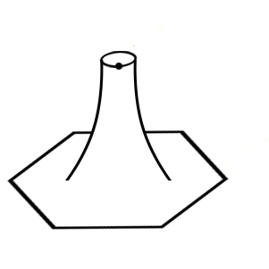
[2] [8.6cm] [8.6cm]

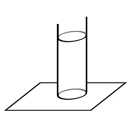
Figure 1. Homomorphism from symplectic homology to the Hochschild cohomology of Fukaya category (Seidel [37]).

Figure 2. Homomorphism from linearized contact homology to the $S^{1}$-equivariant homology of the free loop space of the zero section (Cieliebak-Latschev [12]).

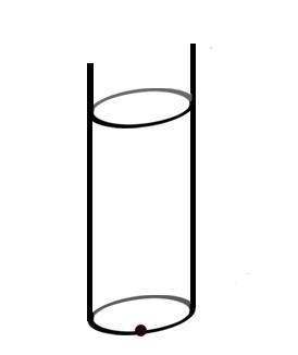
[2] [8.6cm] [8.6cm]

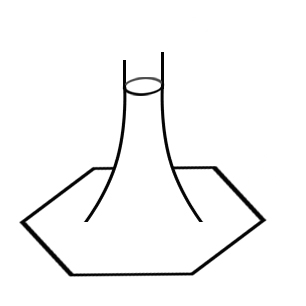
Figure 3. Homomorphism from $S^{1}$-parametrized linearized contact homology to symplectic homology (Bourgeois-Oancea [7]).

Figure 4. Homomorphism in current paper from linearized contact homology to the cyclic cohomology of Fukaya category.

Also, after the first draft was posted on arXiv, we are informed by Eliashberg that he, Bourgeois and Ekholm have obtained some results analogous to ours ([3, 4]). In these two papers they study a variety of algebraic structures (including Lie bialgebra) on the Legendrian homology, and relate them to symplectic homology (the pictures are similar to above). We are grateful to him for acknowledging us about their work.

1.3.

The rest of the paper is devoted to the proof of the above theorems. It is organized as follows: In §2, we first collect some facts on the Fukaya category of exact symplectic manifolds, and then prove Theorem A in §2.3. In §3 we recall the definition and some properties of linearized contact homology. In §4 we set up the necessary analytic machinery for the moduli space of pseudo-holomorphic curves to be considered later. In §5 we prove Theorem B. In §6, we study the example of cotangent bundles and relate it with string topology.

1.4.

Finally, we remark that in this article, TCFT and string topology have served as an inspiring motivation of our study. However, the main body of this article is independent of these two theories, and we shall not discuss any details of them in the rest of the paper. The interested reader may refer to the literature.

Acknowledgements.

Some results in this paper have been presented by the first author at the Chern Institute, Tianjin in 2010 and on the Sullivanfest, Stony Brook in 2011; he would like to thank these two places for their hospitalities. The first author also thanks Nanjing Normal University, the Capital Normal University and NCTS in Taiwan for their supports and hospitalities, and Liang Kong for very inspiring conversations. The second author would like to thank BICMR and the Capital Normal University for their hospitalities, and Gang Tian for helpful suggestions. All three authors thank Yiming Long and Yongbin Ruan for their encouragements during these years, and D. Pomerleano for pointing out an error in previous draft.

2. Fukaya category of exact symplectic manifolds

2.1. A_∞ categories

Definition 1 (A_∞ Category).

An A_∞ category $\mathcal{A}$ consists of a set of objects $\mathcal{O}b(\mathcal{A})$, a graded vector space $\mathrm{Hom}_{\mathcal{A}}(A_{1},A_{2})$ for each pair of objects $A_{1},A_{2}\in\mathcal{O}b(\mathcal{A})$, and a sequence of operators:

$$m_{n}^{\mathcal{A}}:\mathrm{Hom}_{\mathcal{A}}(A_{1},A_{2})\otimes\mathrm{Hom}_{\mathcal{A}}(A_{2},A_{3})\otimes\cdots\otimes\mathrm{Hom}_{\mathcal{A}}(A_{n},A_{n+1})\to\mathrm{Hom}_{\mathcal{A}}(A_{1},A_{n+1}),$$

where $|m_{n}^{\mathcal{A}}|=2-n$, for $n=1,2,\cdots,$ satisfying the following A_∞ relations:

$$\sum_{p=1}^{n}\sum_{k=1}^{n-p+1}(-1)^{\mu_{npk}}m_{n-k+1}^{\mathcal{A}}(a_{1},\cdots,a_{p-1},m_{k}^{\mathcal{A}}(a_{p},\cdots,a_{p+k-1}),a_{p+k},\cdots,a_{n})=0,$$ (2)

where $a_{i}\in\mathrm{Hom}_{\mathcal{A}}(A_{i},A_{i+1})$, for $i=1,2,\cdots,n$, and $\mu_{npk}=\sum\limits_{r=1}^{n}(r-1)|a_{r}|+\sum\limits_{s=1}^{p-1}k|a_{s}|+p(2-k)$.

If an A_∞ category has one object, say $A$, then $\mathrm{Hom}_{\mathcal{A}}(A,A)$ is an A_∞ algebra; and if furthermore, all $m_{i}$, $i\geq 3$, vanish, then $\mathcal{A}$ is the usual differential graded (DG) algebra.

Convention (The Sign Rule).

The sign in equation (2) is always complicated. The rule is given as follows. First, for a graded vector space $V$, let $\overline{V}$ be the desuspension of $V$, that is, $(\overline{V})_{i}=V_{i+1}$. Let $\Sigma:V\to\overline{V}$ be the identity map which maps $v$ to $\overline{v}$, and let

$$\begin{array}[]{cccl}\Sigma^{\otimes n}:&V\otimes\cdots\otimes V&\longrightarrow&\overline{V}\otimes\cdots\otimes\overline{V}\\ &v_{1}\otimes\cdots\otimes v_{n}&\longmapsto&(-1)^{(n-1)|v_{1}|+\cdots+|v_{n-1}|}\overline{v}_{1}\otimes\cdots\otimes\overline{v}_{n}\end{array}$$

be the $n$-folder tensor of $\Sigma$. Let $\overline{m}_{n}:(\overline{V})^{\otimes n}\to\overline{V}$ be the degree 1 map such that the diagram

(3)

commutes. Then equation (2) is nothing but

$$\sum_{p=1}^{n}\sum_{k=1}^{n-p+1}(-1)^{|\overline{a}_{1}|+\cdots+|\overline{a}_{p-1}|}\overline{m}_{n-k+1}(\overline{a}_{1},\cdots,\overline{a}_{p-1},\overline{m}_{k}(\overline{a}_{p},\cdots,\overline{a}_{p+k-1}),\overline{a}_{p+k},\cdots,\overline{a}_{n})=0.$$ (4)

The sign that appears in equation (4) follows from the usual Koszul convention rule. Namely, the canonical isomorphism $V\otimes W\stackrel{{\scriptstyle\cong}}{{\to}}W\otimes V$ is given by $a\otimes b\mapsto(-1)^{|a||b|}b\otimes a$. One then obtains equation (2) by converting equation (4) via diagram (3). In the following all signs are assigned in this way, and therefore we will just simply write $\pm$, without specifying their particular value.

In the following, if $\mathcal{A}$ is clear from the context, we will simply write $\mathrm{Hom}_{\mathcal{A}}(A,B)$ and $m_{i}^{\mathcal{A}}$ as $\mathrm{Hom}(A,B)$ and $m_{i}$. For an A_∞ category $\mathcal{A}$, since $m_{1}\circ m_{1}=0$, one obtains the cohomological category ${\mathrm{H}}(\mathcal{A})$ of $\mathcal{A}$. Namely, the objects of ${\mathrm{H}}(\mathcal{A})$ are the same as the objects of $\mathcal{A}$ while the morphisms from $A$ to $B$ are the cohomology classes ${\mathrm{H}}(\mathrm{Hom}(A,B),m_{1})$. ${\mathrm{H}}(\mathcal{A})$ is a not-necessarily-unital category.

Definition 2 (Hochschild Homology).

Let $\mathcal{A}$ be an A_∞ category. The Hochschild chain complex $\mathrm{Hoch}_{*}(\mathcal{A})$ of $\mathcal{A}$ is the chain complex whose underlying vector space is

$$\bigoplus_{n=1}^{\infty}\bigoplus_{A_{1},A_{2},\cdots,A_{n+1}\in\mathcal{O}b(\mathcal{A})}\overline{\mathrm{Hom}}(A_{1},A_{2})\otimes\overline{\mathrm{Hom}}(A_{2},A_{3})\otimes\cdots\otimes\overline{\mathrm{Hom}}(A_{n+1},A_{1})$$ (5)

with differential $b$ defined by

$$b(\overline{a}_{1},\overline{a}_{2},\cdots,\overline{a}_{n+1})$$

$$= \sum_{k=1}^{n+1}\sum_{i=1}^{n-k+1}\pm(\overline{a}_{1},\cdots,\overline{a}_{k-1},\overline{m}_{i}(\overline{a}_{k},\cdots,\overline{a}_{k+i-1}),\overline{a}_{k+i},\cdots,\overline{a}_{n+1})$$

$$+ \sum_{j=0}^{n-1}\sum_{i=1}^{n-j}\pm(\overline{m}_{i+j+1}(\overline{a}_{n-j+1},\overline{a}_{n-j+2},\cdots,\overline{a}_{n+1},\overline{a}_{1},\overline{a}_{2},\cdots,\overline{a}_{i}),\overline{a}_{i+1}\cdots,\overline{a}_{n-j}).$$

The associated homology is called the Hochschild homology of $\mathcal{A}$, and is denoted by $\mathrm{HH}_{*}(\mathcal{A})$.

Definition 3 (Cyclic Homology).

Suppose $\mathcal{A}$ is an A_∞ category. Let

$$t_{n}:\overline{\mathrm{Hom}}(A_{1},A_{2})\otimes\overline{\mathrm{Hom}}(A_{2},A_{3})\otimes\cdots\otimes\overline{\mathrm{Hom}}(A_{n+1},A_{1})\\ \longrightarrow\overline{\mathrm{Hom}}(A_{n+1},A_{1})\otimes\overline{\mathrm{Hom}}(A_{1},A_{2})\cdots\otimes\overline{\mathrm{Hom}}(A_{n},A_{n+1}),$$

for $n=0,1,2,\cdots$, be the linear map

$$t_{n}(\overline{a}_{1},\overline{a}_{2},\cdots,\overline{a}_{n+1}):=(-1)^{|\overline{a}_{n+1}|(|\overline{a}_{1}|+\cdots+|\overline{a}_{n}|)}(\overline{a}_{n+1},\overline{a}_{1},\cdots,\overline{a}_{n}).$$ (6)

Extend $t_{n}$ to $\mathrm{Hoch}_{*}(\mathcal{A})$ trivially, and let $t=t_{0}+t_{1}+t_{2}+\cdots$, the cokernel $\mathrm{Hoch}_{*}(\mathcal{A})/(1-t)$ of $1-t$ forms a chain complex with the induced differential from the Hochschild complex (still denoted by $b$). Such chain complex is denoted by $\mathrm{Cycl}_{*}(\mathcal{A})$, and is called the Connes cyclic complex of $\mathcal{A}$. Its homology is called the cyclic homology of $\mathcal{A}$, and is denoted by $\mathrm{HC}_{*}(\mathcal{A})$.

The cyclic cohomology of $\mathcal{A}$ is the homology of the dual cochain complex $\mathrm{Cycl}^{*}(\mathcal{A})$ of $\mathrm{Cycl}_{*}(\mathcal{A})$. Namely, suppose $f\in\mathrm{Hom}(\mathrm{Hoch}_{*}(\mathcal{A}),k)$, then $f\in\mathrm{Cycl}^{*}(\mathcal{A})$ if and only if for all $\alpha\in\mathrm{Hoch}_{*}(\mathcal{A})$, $f(\alpha)=f(t(\alpha))$.

2.2. Review of the Fukaya category

In this subsection we briefly recall the construction of the Fukaya category in exact symplectic manifolds. We adopt the setting of Seidel [38]. All details and proofs are omitted. The construction in a general symplectic manifold is given in Fukaya [17, Chapter 1], largely based on the work [19]; however, we do not need to be such general.

An exact symplectic manifold with contact type boundary is a quadruple $(M,\omega,\eta,J)$, where $M$ is a compact $2n$ dimensional manifold with boundary, $\omega$ is a symplectic 2-form on $M$, $\eta$ is a 1-form such that $\omega=d\eta$ and $J$ is a $\omega$-compatible almost complex structure. These data also satisfy the following two convexity conditions:

• The negative Liouville vector field defined by $\omega(\cdot,X_{\eta})=\eta$ points strictly inwards along the boundary of $M$;

• The boundary of $M$ is weakly $J$-convex, which means that any pseudo-holomorphic curves cannot touch the boundary unless they are completely contained in it.

An $n$ dimensional submanifold $L\subset M$ is called Lagrangian if $\omega|L=0$. We always assume $L$ is closed and is disjoint from the boundary of $M$. $L$ is called exact if $\eta|L$ is an exact 1-form.

Assumption 4.

In the following, for a symplectic manifold $M$ with or without (contact type) boundary, we shall always assume $c_{1}(M)=0$, and for a Lagrangian submanifold $L$ in $M$, we shall always assume it is admissible, namely, (1) $\eta|_{L}$ is exact; (2) $L$ has vanishing Maslov class; and (3) $L$ is spin.

Example 5 (Cotangent Bundles).

Let $N$ be a simply connected, compact spin manifold. Let $T^{*}N$ be the cotangent bundle of $N$ with the canonical symplectic structure. The cotangent disk bundle of $N$ is an exact symplectic with contact type boundary. In particular, $N$, viewed as the zero section of $T^{*}N$, is an admissible Lagrangian submanifold.

Intuitively, the Fukaya category $\mathcal{F}uk(M)$ of $M$ is defined as follows: the objects are the admissible Lagrangian submanifolds; suppose $L_{1},L_{2}$ are two objects, $\mathrm{Hom}(L_{1},L_{2})$, called the Floer cochain complex, is spanned by the transversal intersection points of $L_{1}$ and $L_{2}$, and for $n$ objects $L_{1},\cdots,L_{n+1}$,

$$\overline{m}_{n}:\overline{\mathrm{Hom}}(L_{1},L_{2})\otimes\overline{\mathrm{Hom}}(L_{2},L_{3})\otimes\cdots\otimes\overline{\mathrm{Hom}}(L_{n},L_{n+1})\to\overline{\mathrm{Hom}}(L_{1},L_{n+1})$$

is given by counting pseudo-holomorphic disks whose boundary lying in $L_{1},L_{2},\cdots,L_{n+1}$. More precisely, if $a_{1}\in\mathrm{Hom}(L_{1},L_{2}),\cdots,a_{n}\in\mathrm{Hom}(L_{n},L_{n+1})$,

$$\overline{m}_{n}(\overline{a}_{1},\overline{a}_{2},\cdots,\overline{a}_{n})=\sum_{a\in L_{1}\cap L_{n+1}}\#(\mathcal{M}(a,a_{1},\cdots,a_{n}))\cdot\overline{a},$$

where $\mathcal{M}(a,a_{1},\cdots,a_{n})$ is the moduli space of pseudo-holomorphic disks with $n+1$ (anti-clockwise) cyclically ordered marked points in its boundary, such that these marked points are mapped onto $a,a_{n},\cdots,a_{1}$ and that the rest of the boundary lie in $L_{1},L_{2},\cdots,L_{n+1}$. The A_∞ relations (equation (2)) follow from the compactification of $\mathcal{M}(a,a_{1},\cdots,a_{n})$ where those pseudo-holomorphic disks with all possible “bubbling-off” disks are added.

This is a very rough description of the construction of the Fukaya category. It is only partially defined in the sense that we have assumed that all Lagrangian submanifolds are transversal; also, the Floer cochains thus described are only $\mathbb{Z}_{2}$ graded. To make the Fukaya category be fully defined and be graded over $\mathbb{Z}$, we have to introduce the following concepts. Let us do it one by one.

2.2.1. Pointed-boundary Riemann surfaces

Suppose $\widehat{S}$ be a Riemann surface with boundary, and $\Sigma$ is a set of boundary points in $\widehat{S}$. $\Sigma$ is divided into two subsets $\Sigma^{+}$ and $\Sigma^{-}$, called the output subset and input subset. Now to each $\zeta\in\Sigma$, one associates:

• two admissible Lagrangian submanifolds $(L_{\zeta 0},L_{\zeta 1})$, where $L_{\zeta 0}$ is uniquely attached to the boundary component of $S:=\widehat{S}\backslash\Sigma$ that comes before $\zeta$ and $L_{\zeta 1}$ is uniquely attached to the boundary component (with induced orientation) that comes after $\zeta$ if $\zeta\in\Sigma^{+}$; otherwise if $\zeta\in\Sigma^{-}$, $L_{\zeta 1}$ comes before $L_{\zeta 0}$. These Lagrangian submanifolds are called the Lagrangian labels.

• a strip-like end which is a proper holomorphic embedding $\epsilon_{\zeta}:Z^{\pm}\to S$ satisfying

  $$\epsilon^{-1}_{\zeta}(\partial S)=\mathbb{R}^{\pm}\times\{0,1\}\ \ \ {\rm and} \ \ \ \lim_{s\to\pm\infty}\epsilon_{\zeta}(s,\cdot)=\zeta,$$ (7)

  where $Z^{\pm}=\mathbb{R}^{\pm}\times[0,1]$ denotes the semi-infinite strips. If $\Sigma$ consists of more than one point, we also need the additional requirement that the images of the $\epsilon_{\zeta}$ are pairwise disjoint. Such an $S$ is called a pointed-boundary Riemann surface with strip-like ends.

2.2.2. Floer data and perturbation data

Suppose $(M,\omega,J)$ is an exact symplectic manifold with contact type boundary. Let $\mathscr{J}$ be the space of all $\omega$-compatible almost complex structures on $M$ which agree with the given $J$ near the boundary; and let $\mathscr{H}=C_{c}^{\infty}(int(M),\mathbb{R})$ be the space of smooth functions on $M$ vanishing near the boundary.

Definition 6 (Floer Datum).

For each ordered pair of Lagrangian submanifolds $L_{0},L_{1}\subset M$, a Floer datum consists of $H_{L_{0},L_{1}}\in C^{\infty}([0,1],\mathscr{H})$ and $J\in C^{\infty}([0,1],\mathscr{J})$, with the following property: if $X$ is the time-dependent Hamiltonian vector field of $H$ and $\phi$ is its flow, then $\phi^{1}(L_{0})$ intersects $L_{1}$ transversally.

Definition 7 (Perturbation Datum).

Let $S$ be a pointed-boundary Riemann surface with Lagrangian labels. Suppose we have chosen strip-like ends for it, and also a Floer datum $(H_{\zeta},J_{\zeta})$ for each of the pairs of sub manifolds $(L_{\zeta 0},L_{\zeta 1})$ associated to the points at infinity $\zeta\in\Sigma$. A perturbation datum for $S$ is a pair $(K,J)$ where

• $K\in\Omega^{1}(S,\mathscr{H})$ satisfies $K(\xi)|L_{C}=0$, for all $\xi\in TC$, where $C$ is a component of $\partial S$, and

• $J$ is a family of almost complex structures $J\in C^{\infty}(S,\mathscr{J})$,

such that they are compatible with the chosen strip-like ends and Floer data, in the sense that

$$\epsilon^{*}_{\zeta}K=H_{\zeta}(t)dt,\quad J(\epsilon_{\zeta}(s,t))=J_{\zeta}(t)$$

for each $\zeta\in\Sigma^{\pm}$ and $(s,t)\in Z^{\pm}$.

For convenience, we call a Floer datum together with a perturbation datum the analytic data, and denote it by $\mathbf{D}_{\mathrm{Fuk}}$.

2.2.3. Grading of Lagrangian submanifolds

Let $(\mathbb{R}^{2n},\omega)$ be the standard symplectic vector space. Denote by ${Lag}_{n}={Lag}(\mathbb{R}^{2n},\omega)$ the set of all linear Lagrangian subspaces. It is known that $\pi_{1}({Lag}_{n})\cong\mathbb{Z}$ (c.f. [33, Theorem 2.31]). Denote by $\widetilde{{Lag}}_{n}$ the universal covering of ${Lag}_{n}$.

Now suppose $(M^{2n},\omega)$ is a symplectic manifold, then to each $p\in M$ is associated ${Lag}(T_{p}M)$, and one obtains a fiber bundle, denoted by ${Lag}(M)\to M$.

Lemma 8.

There exists a covering $\widetilde{{Lag}}(M)$ of ${Lag}(M)$ such that its restriction to each fiber is identified with $\widetilde{{Lag}}_{n}\to{Lag}_{n}$ if and only if $c_{1}(M)=0$.

Proof.

See Fukaya [17, Lemma 2.6]. ∎

From now on we fix a covering $\widetilde{{Lag}}(M)$ as in the above lemma. Now suppose $L$ is a Lagrangian submanifold; then there is a canonical section $s$ of the restriction of ${Lag}(M)$ to $L$, which is given by $s(p)=T_{p}L\subset T_{p}M$.

Definition 9 (Grading of Lagrangian Submanifolds).

A graded Lagrangian submanifold of $(M,\widetilde{{Lag}}(M))$ is an oriented Lagrangian submanifold $L$ and a lift of $s$ to $\tilde{s}:L\to\widetilde{{Lag}}(M)$. The lifting $\tilde{s}$ is called the grading of $L$, and denote $L$ with $\tilde{s}$ by $\tilde{L}$.

The grading of a Lagrangian submanifold is related to its Maslov class as follows: Let $\phi:(D^{2},\partial D^{2})\to(M,L)$ be a map representing $\pi_{2}(M,L)$. For each $t\in\partial D^{2}$ we have a Lagrangian subspace $T_{\phi(t)}L\subset T_{\phi(t)}M$, which gives a map $S^{1}\to{Lag}_{n}$. It determines an element in $\pi_{1}({Lag}_{n})\cong\mathbb{Z}$, which is called the Maslov index of $[\phi]$, and is denoted by $\mu([\phi])$. Under the assumption that $c_{1}(M)=0$, $\mu$ can be extended to $\pi_{1}(L)$ as follows: By Lemma 8 there exist a lift $\widetilde{{Lag}}(M)\to M$. Let $\gamma:S^{1}\to L$ be a representation of an element of $\pi_{1}(L)$. Define a map $\gamma^{+}:S^{1}\to{Lag}(M)$ by

$$\gamma^{+}(t)=T_{\gamma(t)}L\in{Lag}(T_{p}M).$$

Since $\widetilde{{Lag}}(M)\to{Lag}(M)$ is a covering, we have a lift $\tilde{\gamma}^{+}:[0,1]\to\widetilde{{Lag}}(M)$ of $\gamma^{+}$. By the fact that $\widetilde{{Lag}}_{n}/{\mathbb{Z}}={Lag}_{n}$ there exists $\overline{\mu}(\gamma)\in{\mathbb{Z}}$ such that

$$\overline{\mu}(\gamma)\cdot\tilde{\gamma}^{+}(0)=\tilde{\gamma}^{+}(1).$$

The map $\overline{\mu}:\pi_{1}(L)\to{\mathbb{Z}}$ is called the Maslov class of $L$. We have:

Lemma 10.

Suppose $c_{1}(M)=0$, then there exists a lift $\tilde{s}$ of $s:L\to{Lag}(M)$ if and only if the Maslov class $\overline{\mu}:\pi_{1}(L)\to{\mathbb{Z}}$ is zero.

Proof.

See Fukaya [17, Lemma 2.14]. ∎

2.2.4. Definition of a Floer cochain

Suppose $\tilde{L}_{1},\tilde{L}_{2}$ intersect transversally and $p\in\tilde{L}_{1}\cap\tilde{L}_{2}$; we next define a grading $\eta_{\tilde{L}_{1},\tilde{L}_{2}}(p)$ for $p$. Let

$$Y:=D^{2}\cup\{x+y\sqrt{-1}|x\geq 0,y\in[-1,1]\}\subset\mathbb{C}.$$

The boundary $\partial Y$ is identified with $\mathbb{R}$ where $\infty-\sqrt{-1}$ corresponds to $-\infty$ and $\infty+\sqrt{-1}$ corresponds to $+\infty$. Define a path $\tilde{l}:\mathbb{R}\to\widetilde{{Lag}}(T_{p}M)$ such that $\tilde{l}(-\infty)=\tilde{s}_{1}(p)$ and $\tilde{l}(\infty)=\tilde{s}_{2}(p)$, where $\tilde{s}_{1}$ and $\tilde{s}_{2}$ are the gradings of the Lagrangian submanifolds $L_{1}$ and $L_{2}$. Assume that $\tilde{l}(t)$ is locally constant if $|t|>T$.

Lemma 11.

Let $l=\pi\circ\tilde{l}$ and $W^{1,k}(Y,T_{p}M;l):=\{u\in W^{1,k}(Y,T_{p}M)|u(x)\in l(x)~{}\mbox{if }~{}x\in\partial Y\cong\mathbb{R}\}$. Then

$$\overline{\partial}:W^{1,k}(Y,T_{p}M;l)\to W^{0,k}(Y,T_{p}M\otimes\Lambda^{0,1})$$ (8)

is a Fredholm operator.

Proof.

See Fukaya [17, Lemma 3.9].∎

Definition 12 (Floer Cochain).

If $\tilde{L}_{1},\tilde{L}_{2}$ intersect transversally, then the grading $\eta_{\tilde{L}_{1},\tilde{L}_{2}}(p)$ of $p$ is defined to be the index of $\overline{\partial}$ in above lemma. More generally, for two arbitrary $\tilde{L}_{1},\tilde{L}_{2}$ with analytic data, let

$$\mathrm{Hom}(\tilde{L}_{1},\tilde{L}_{2}):=\mbox{Span}\{y:[0,1]\to M|y(0)\in L_{1},y(1)\in L_{2},\mbox{ and }dy/dt=X(t,y(t))\}.$$ (9)

where the grading of $y$, when viewed as the intersection point $p$ of $\tilde{L}_{1},\phi(\tilde{L}_{2})$, is defined to be the grading $\eta_{\tilde{L}_{1},\phi(\tilde{L}_{2})}(p)$. An element in $\mathrm{Hom}(\tilde{L}_{1},\tilde{L}_{2})$ is called a Floer cochain of $\tilde{L}_{1}$ and $\tilde{L}_{2}$, and $y$ is sometimes called a Hamiltonian chord.

Lemma 13.

If $\tilde{L}_{1},\tilde{L}_{2}$ intersect transversally, then one may choose $H_{L_{0},L_{1}}$ to be zero, and $p\in\mathrm{Hom}(\tilde{L}_{1},\tilde{L}_{2})$ implies the same $p$ lies in $\mathrm{Hom}(\tilde{L}_{2},\tilde{L}_{1})$; to distinguish, we write $p^{*}\in\mathrm{Hom}(\tilde{L}_{2},\tilde{L}_{1})$. We have

$$\eta_{\tilde{L}_{0},\tilde{L}_{1}}(p)+\eta_{\tilde{L}_{1},\tilde{L}_{0}}(p^{*})={\dim M}/{2}.$$

Proof.

See Fukaya [17, Lemma 2.27]. ∎

2.2.5. Moduli space of pseudo-holomorphic disks

Take a pointed-boundary disk $S$ with Lagrangian labels. Equip it with strip-like ends, Floer data $(H_{\zeta},J_{\zeta})$ for each point at infinity, and a compatible perturbation datem $(K,J)$. $K$ determines a vector-field-valued 1-form $Y\in\Omega^{1}(S,C^{\infty}(T))$: for each $\xi\in TS$, $Y(\xi)$ is the Hamiltonian vector field of $K(\xi)$. The inhomogeneous pseudo-holomorphic map equation for $u\in C^{\infty}(S,M)$ is

$$\left\{\begin{array}[]{l}Du(z)+J(z,u)\circ Du(z)\circ I_{S}=Y(z,u)+J(z,u)\circ Y(z,u)\circ I_{S},\\ u(C)\subset L_{C}\quad\mbox{for all}\quad C\subset\partial S,\end{array}\right.$$ (10)

where $I_{S}$ is the complex structure on $S$.

By varying the complex structures on $S$ (we require that at infinity the complex structures is fixed), one obtains a universal family of pointed-boundary disks with strip-like ends, equipped with Lagrangian labels. For such a family, one may choose a family of consistent perturbation data (for the existence see Seidel [38, §9i]). Now suppose $a_{1}\in\mathrm{Hom}(\tilde{L}_{1},\tilde{L}_{2}),\cdots,a_{n}\in\mathrm{Hom}(\tilde{L}_{n},\tilde{L}_{n+1}),a_{n+1}\in\mathrm{Hom}(\tilde{L}_{1},\tilde{L}_{n+1})$. Let

$${\mathcal{M}}(a_{1},a_{2},\cdots,a_{n+1}):=\left\{u\in C^{\infty}(S,M)\left|\begin{array}[]{l}u\,\mbox{satisfies~{}(\ref{IHE})\,and the strip-like ends}\\ \mbox{converge to}\,a_{1},\cdots,a_{n+1},\,\mbox{respectively}\end{array}\right.\right\}$$

be the moduli space of solutions to (10).

2.2.6. Compactification and orientation of the moduli spaces

Theorem 14.

${\mathcal{M}}$ admits a natural compactification and orientation.

Proof.

See Seidel [38, §9l].∎

The compactification of $\mathcal{M}(a_{1},a_{2},\cdots,a_{n+1})$ is a smooth stratified space (manifold with corners), where the corners consists of all possible pseudo-holomorphic disks with “bubbling-off” disks. Its codimension one strata consists of

$$\bigcup_{1\leq i<j\leq n+1}\bigcup_{b\in\mathrm{Hom}(\tilde{L}_{i},\tilde{L}_{j-1})}\mathcal{M}(b,a_{i},\cdots,a_{j-1})\times\mathcal{M}(a_{1},\cdots,a_{i-1},b,a_{j},\cdots,a_{n+1}).$$ (11)

The orientation is signed the following way: for each $a_{i}$, let $o_{a_{i}}$ be the determinant bundle $\det\overline{\partial}$ of equation (8); then the orientation bundle of $\mathcal{M}(a_{n+1},a_{1},\cdots,a_{n})$ is

$$o_{a_{n+1}}\otimes o_{a_{1}}^{-}\otimes\cdots\otimes o_{a_{n}}^{-},$$

where $o_{a_{i}}^{-}$ is the dual bundle of $o_{a_{i}}$. Note that, $\mathcal{M}(a_{n+1},a_{1},\cdots,a_{n})$ and $\mathcal{M}(a_{1},\cdots,a_{n},a_{n+1})$ count the same set of pseudo-holomorphic disks, however, their orientations agree if and only if $|a_{n+1}|(|a_{1}|+\cdots+|a_{n}|)$ is even.

2.2.7. Construction of the Fukaya category

Theorem 15.

Suppose $M$ is an exact symplectic manifold with $c_{1}(M)=0$, and possibly with contact type boundary. Suppose $\tilde{L}_{1},\tilde{L}_{2},\cdots,\tilde{L}_{n+1}$ are admissible graded Lagrangian submanifolds, and $a_{i}\in\mathrm{Hom}(\tilde{L}_{i},\tilde{L}_{i+1})$, $i=1,2,\cdots,n$. Define

$$\begin{array}[]{cccl}\overline{m}_{n}:&\overline{\mathrm{Hom}}(\tilde{L}_{1},\tilde{L}_{2})\otimes\cdots\otimes\overline{\mathrm{Hom}}(\tilde{L}_{n},\tilde{L}_{n+1})&\longrightarrow&\overline{\mathrm{Hom}}(\tilde{L}_{1},\tilde{L}_{n+1})\\ &(\overline{a}_{1},\overline{a}_{2},\cdots,\overline{a}_{n})&\longmapsto&\displaystyle\sum_{a\in\mathrm{Hom}(\tilde{L}_{1},\tilde{L}_{n+1})}\#{\mathcal{M}}(a,a_{1},\cdots,a_{n})\cdot\overline{a},\end{array}$$

for $n=1,2,\cdots$. Then the set of admissible Lagrangian submanifolds and the Floer cochain complex among them together with $\{\overline{m}_{n}\}$ defined above form an A_∞ category, called the Fukaya category of $M$, and is denoted by $\mathcal{F}uk(M)$.

This is proved in [38, Chapter II] for the exact case and in [17] for the general case; we will not repeat it. The (ir)relevance of the construction to the choice of the analytic data is also completely discussed in [38, §12]. Such a technical problem will also appear in our case when counting the pseudo-holomorphic disks with punctures. However, all Seidel’s argument can be applied to our case, and we will not address this issue in current paper.

2.2.8. Cyclicity and a strengthening of the analytic data

From Seidel’s original definition, one sees that:

• if $L_{0},L_{1}$ intersect transversally, then one may choose $H_{L_{0},L_{1}}=0$, and up to a degree shifting $\mathrm{Hom}(\tilde{L}_{0},\tilde{L}_{1})\cong\mathrm{Hom}(\tilde{L}_{1},\tilde{L}_{0})$ (see Lemma 13); however,

• if $L_{0},L_{1}$ do not intersect transversally, then $H_{L_{0},L_{1}}$ does not vanish, and therefore $\mathrm{Hom}(\tilde{L}_{0},\tilde{L}_{1})$ is by no means the same as $\mathrm{Hom}(\tilde{L}_{1},\tilde{L}_{0})$.

To overcome this inconsistency, i.e. to make Lemma 13 hold even for non transversal pair of Lagrangian submanifolds, we make the following additional condition for the Floer data:

Definition 16 (Modified Floer Datum).

For each ordered pair of Lagrangian submanifolds $L_{0},L_{1}\subset M$, a Floer datum consists of $H_{L_{0},L_{1}}\in C^{\infty}([0,1],\mathscr{H})$ and $J\in C^{\infty}([0,1],\mathscr{J})$, besides the requirement of Definition 6, satisfying the following additional properties:

1. for the opposite ordered pair $(L_{1},L_{0})$, $H_{L_{1},L_{0}}(t)=-H_{L_{0},L_{1}}(1-t)$;

2. if $X$ is the time-dependent Hamiltonian vector field of $H_{L_{0},L_{1}}$ and $\phi_{X}$ its flow, then $\phi^{1/2}_{X(t)}(L_{0})$ intersects $\phi^{1/2}_{-X(1-t)}(L_{1})$ transversally. (Note $-X(1-t)$ is the Hamiltonian vector field of $H_{L_{1},L_{0}}$.)

The perturbation data will be changed accordingly. With such a modification, one sees that in the case when $L_{0}$ and $L_{1}$ do not intersect transversally, the generators of $\mathrm{Hom}(\tilde{L}_{0},\tilde{L}_{1})$ and $\mathrm{Hom}(\tilde{L}_{1},\tilde{L}_{0})$ may both be identified with the intersection points of $\phi^{1/2}_{X}(L_{0})$ and $\phi^{1/2}_{-X}(L_{1})$, and the degrees at each point add up to $n$. An application of this is the Lie bialgebra structure on the cyclic complex of the Fukaya category, which we discuss in the next subsection.

2.3. The Lie bialgebra structure

From now on, we graded the Floer cochains negatively. Such a convention is usually adopted in algebraic topology when studying Hochschild/cyclic homology of the cochain complex of topological spaces.

Definition 17 (Lie Bialgebra).

Let $L$ be a (possibly graded) $\mathbb{K}$-space. A Lie bialgebra on $L$ is the triple $(L,[\,,\,],\delta)$ such that

• $(L,[\,,\,])$ is a Lie algebra;

• $(L,\delta)$ is a Lie coalgebra;

• The Lie algebra and coalgebra satisfy the following identity, called the Drinfeld compatibility:

  $$\delta[a,b]=\sum_{(a)}((-1)^{|a^{\prime\prime}||b|}[a^{\prime},b]\otimes a^{\prime\prime}+a^{\prime}\otimes[a^{\prime\prime},b])+\sum_{(b)}([a,b^{\prime}]\otimes b^{\prime\prime}+(-1)^{|a||b^{\prime}|}b^{\prime}\otimes[a,b^{\prime\prime}]),$$

  for all $a,b\in L$, where we write $\delta(a)=\sum_{(a)}a^{\prime}\otimes a^{\prime\prime}$ and $\delta(b)=\sum_{(b)}b^{\prime}\otimes b^{\prime\prime}$.

If moreover, $[\,,\,]\circ\delta(a)\equiv 0$, for all $a\in L$, $(L,[\,,\,],\delta)$ is said to be involutive. If the Lie bracket has degree $k$ and the Lie cobracket has degree $l$, denote the Lie bialgebra with degree $(l,k)$.

Theorem 18 (Lie Bialgebra of The Fukaya Category).

Let $M^{2n}$ be an exact symplectic manifold (possibly with contact type boundary) with $c_{1}(M)=0$. Grade the Floer cochain complex negatively. Then the cyclic cochain complex of the Fukaya category $\mathcal{F}uk(M)$ of $M$ has the structure of a differential involutive Lie bialgebra of degree $(2-n,2-n)$.

The proof of this theorem consists of the rest of the subsection. Before going to the details, we would like to say several words about the degrees. We say a graded vector space $V$ is a Lie algebra of degree $n$ if $V[-n]$ is a graded Lie algebra in the usual sense. Similar convention applies to Lie bialgebras with a bi-degree $(m,n)$. A technical issue here is the correctness of Drinfeld compatibility and involutivity. In our case of the Lie bialgebra of degree $(2-n,2-n)$, if we shift the vector space down by $2-n$, then the Lie bracket has degree zero and the Lie cobracket has degree $4-2n$, which is even. Therefore, equations for the Drinfeld compatibility and involutivity in this case is the same as in the usual case.

Lemma 19 (Lie Algebra).

Denote by $\mathcal{F}uk(M)$ the Fukaya category of $M$. Define

$$[\,,\,]:\mathrm{Cycl}^{*}(\mathcal{F}uk(M))\otimes\mathrm{Cycl}^{*}(\mathcal{F}uk(M))\to\mathrm{Cycl}^{*}(\mathcal{F}uk(M))$$

by

$$[f,g](\overline{a}_{1},\overline{a}_{2},\cdots,\overline{a}_{n}) := \sum_{i<j}\sum_{p\in\mathrm{Hom}(\tilde{L}_{j},\tilde{L}_{i})}\pm f(\overline{a}_{i},\cdots,\overline{a}_{j-1},\overline{p})\cdot g(\overline{p}^{*},\overline{a}_{j},\cdots,\overline{a}_{n},\overline{a}_{1},\cdots,\overline{a}_{i-1})$$

$$- \sum_{i<j}\sum_{p\in\mathrm{Hom}(\tilde{L}_{j},\tilde{L}_{i})}\pm g(\overline{a}_{i},\cdots,\overline{a}_{j-1},\overline{p})\cdot f(\overline{p}^{*},\overline{a}_{j},\cdots,\overline{a}_{n},\overline{a}_{1},\cdots,\overline{a}_{i-1}).$$

Then $(\mathrm{Cycl}^{*}(\mathcal{F}uk(M)),[\,,\,],b)$ forms a differential graded Lie algebra of degree $2-n$.

Pictorially, the bracket is defined as in the following picture (Figure 5):

Figure 5. Definition of the Lie bracket for two cyclic cochains

in the picture, the left side of the equality is the value of $[f,g]$ on $(a_{1},\cdots,a_{n})$, and the right side of the equality is summarized over all possibilities of the product of the value of $f$ on $(a_{i},\cdots,a_{j-1},p)$ with the value of $g$ on $(p^{*},a_{j},\cdots,a_{i-1})$.

Proof.

First, we show $[\,,\,]$ has degree $2-n$. Note that $(\overline{a}_{1},\cdots,\overline{a}_{n})$ has degree

$$|a_{1}|+\cdots+|a_{n}|+n,$$

(recall that we grade $a_{i}\in\mathrm{Hom}(\tilde{L}_{i},\tilde{L}_{i+1})$ negatively). And the sum of the degrees of $(\overline{a}_{i},\cdots,\overline{a}_{j-1},\overline{p})$ and $(\overline{p}^{*},\overline{a}_{j},\cdots,\overline{a}_{n},\cdots,\overline{a}_{i-1})$ is

$$|a_{1}|+\cdots+|a_{n}|+|p|+|p^{*}|+(n+2)$$

$$= |a_{1}|+\cdots+|a_{n}|+|p|+(-n-|p|)+(n+2)\quad(\mbox{recall that}~{}|p^{*}|+|p|=-n)$$

$$= |a_{1}|+\cdots+|a_{n}|+n+(2-n).$$

The difference of these two degrees is exactly $n-2$. Going to the cyclic cochain (i.e. the dual space) level, the degree of the bracket $[\,,\,]$ becomes $2-n$.

Second, we show $[\,,\,]$ is graded skew-symmetric. Observe that in the definition of $[\,,\,]$, if we switch $f$ and $g$, we get exactly the opposite sign (ignoring the intrinsic signs that come from the Koszul convention).

Third, we show the Jacobi identity: With Figure 5 in mind, the value of $[[f,g],h]$ on $(\overline{a}_{1},\cdots,\overline{a}_{n})$ has four terms which can be pictorially represented by the following picture

Similarly, $[[g,h],f]$ and $[[h,f],g]$ are represented by the following picture:

The sum is identically zero, which proves the (graded) Jacobi identity.

Finally, we show that the bracket commutes with the boundary:

$$(b[f,g])(\overline{a}_{1},\overline{a}_{2},\cdots,\overline{a}_{n})$$ (12)

$$= [f,g](b(\overline{a}_{1},\overline{a}_{2},\cdots,\overline{a}_{n}))$$

$$= [f,g]\big{(}\sum_{i}\sum_{k}\pm(\overline{a}_{1},\cdots,\overline{m}_{k}(\overline{a}_{i},\cdots,\overline{a}_{i+k-1}),\cdots,\overline{a}_{n})\big{)}$$

$$+ [f,g]\big{(}\sum_{j}\sum_{k}\pm(\overline{m}_{k}(\overline{a}_{n-j},\cdots,\overline{a}_{n},\overline{a}_{1},\cdots,\overline{a}_{i}),\cdots,\overline{a}_{n-j-1})\big{)},$$ (13)

while

$$([bf,g]+(-1)^{|f|}[f,bg])(\overline{a}_{1},\overline{a}_{2},\cdots,\overline{a}_{n})$$ (14)

$$= \sum_{i<j}\sum_{p}\pm f(b(\overline{a}_{i},\cdots,\overline{a}_{j-1},\overline{p}))\cdot g(\overline{p}^{*},\overline{a}_{j},\cdots,\overline{a}_{i-1})$$

$$- \sum_{i<j}\sum_{p}\pm g(\overline{a}_{i},\cdots,\overline{a}_{j-1},\overline{p})\cdot f(b(\overline{p}^{*},\overline{a}_{j},\cdots,\overline{a}_{i-1}))$$ (15)

$$+ \sum_{i<j}\sum_{p}\pm f(\overline{a}_{i},\cdots,\overline{a}_{j-1},\overline{p})\cdot g(b(\overline{p}^{*},\overline{a}_{j},\cdots,\overline{a}_{i-1}))$$ (16)

$$- \sum_{p}\pm g(b(\overline{a}_{i},\cdots,\overline{a}_{j-1},\overline{p}))\cdot f(\overline{p}^{*},\overline{a}_{j},\cdots,\overline{a}_{i-1}).$$ (17)

From the definition of $[\,,\,]$, one sees $(\ref{Eq_2})+(\ref{Eq_22})+(\ref{Eq_3})+(\ref{Eq_32})$ contains more terms than $(\ref{Eq_1'})+(\ref{Eq_1''})$, namely, those terms involving $\overline{m}_{k}$ acting on $\overline{p}$ and $\overline{p}^{*}$. For example, the extra terms coming from $(\ref{Eq_2})$ are

$$\sum_{p\in\mathrm{Hom}(\tilde{L}_{j},\tilde{L}_{i})}\sum_{k}\sum_{r}f(\overline{m}_{r}(\overline{a}_{k},\cdots,\overline{a}_{j-1},\overline{p},\overline{a}_{i},\cdots,\overline{a}_{l}),\overline{a}_{l+1},\cdots,\overline{a}_{k-1})\cdot g(\overline{p}^{*},\overline{a}_{j},\cdots,\overline{a}_{i-1})$$ (18)

and the ones from $(\ref{Eq_3})$ are

$$\sum_{p\in\mathrm{Hom}(\tilde{L}_{j},\tilde{L}_{i})}\sum_{k}\sum_{r}f(\overline{a}_{i},\cdots,\overline{a}_{j},\overline{p})\cdot g(\overline{m}_{r}(\overline{a}_{k},\cdots,\overline{a}_{i-1},\overline{p}^{*},\overline{a}_{j},\cdots,\overline{a}_{l}),\overline{a}_{l+1},\cdots,\overline{a}_{k-1}).$$ (19)

However, these two groups of terms cancel with each other because

$$\sum_{p\in\mathrm{Hom}(\tilde{L}_{j},\tilde{L}_{i})}\overline{m}_{r}(\overline{a}_{k},\cdots,\overline{a}_{j},\overline{p},\overline{a}_{i},\cdots,\overline{a}_{l})\otimes\overline{p}^{*}$$

$$= \sum_{p\in\mathrm{Hom}(\tilde{L}_{j},\tilde{L}_{i})}\sum_{q\in\mathrm{Hom}(\tilde{L}_{k},\tilde{L}_{l+1})}\#\mathcal{M}(q,a_{k},\cdots,a_{j},p,a_{i},\cdots,a_{l})\overline{q}\otimes\overline{p}^{*}$$

$$= \sum_{q\in\mathrm{Hom}(\tilde{L}_{k},\tilde{L}_{l+1})}\sum_{p\in\mathrm{Hom}(\tilde{L}_{j},\tilde{L}_{i})}\overline{q}\otimes\#\mathcal{M}(q,a_{k},\cdots,a_{j},p,a_{i},\cdots,a_{l})\overline{p}^{*}$$

$$\stackrel{{\scriptstyle\mbox{\scriptsize cyclicity}}}{{=}} \sum_{q\in\mathrm{Hom}(\tilde{L}_{k},\tilde{L}_{l+1})}\sum_{p\in\mathrm{Hom}(\tilde{L}_{j},\tilde{L}_{i})}\overline{q}\otimes\#\mathcal{M}(p,a_{i},\cdots,a_{l},q,a_{k},\cdots,a_{j})\overline{p}^{*}$$

$$\stackrel{{\scriptstyle\S\ref{subsect_cycl}}}{{=}} \sum_{q\in\mathrm{Hom}(\tilde{L}_{k},\tilde{L}_{l+1})}\sum_{p^{*}\in\mathrm{Hom}(\tilde{L}_{i},\tilde{L}_{j})}\overline{q}\otimes\#\mathcal{M}(p^{*},a_{i},\cdots,a_{l},q^{*},a_{k},\cdots,a_{j})\overline{p}^{*}$$

$$= \sum_{q\in\mathrm{Hom}(\tilde{L}_{k},\tilde{L}_{l+1})}\overline{q}\otimes\overline{m}_{r}(\overline{a}_{i},\cdots,\overline{a}_{l},\overline{q}^{*},\overline{a}_{k},\cdots,\overline{a}_{j}).$$

By substituting the above identity into (18) we get exactly (19). Similarly, the extra terms in (15) and in (17) cancel with each other. Pictorially, the value of $b[f,g]$ on $(a_{1},\cdots,a_{n})$ equals

and the value of $[bf,g]+[f,bg]$ on $(a_{1},\cdots,a_{n})$ not only contains the above four terms, but also

which cancel each other within themselves. ∎

Lemma 20 (Lie Coalgebra).

Denote by $\mathcal{F}uk(M)$ the Fukaya category of $M$. Define $\mathrm{Cycl}^{*}(\mathcal{F}uk(M))\to\mathrm{Cycl}^{*}(\mathcal{F}uk(M))\otimes\mathrm{Cycl}^{*}(\mathcal{F}uk(M))$ by

$$(\delta f)(\overline{a}_{1},\overline{a}_{2},\cdots,\overline{a}_{n})\otimes(\overline{b}_{1},\overline{b}_{2},\cdots,\overline{b}_{m})$$

$$:= \sum_{i=1}^{n}\sum_{j=1}^{m}\sum_{p\in\mathrm{Hom}(\tilde{L}_{i},\tilde{L}_{j})}\pm f(\overline{a}_{1},\cdots,\overline{a}_{i-1},\overline{p},\overline{b}_{j},\cdots,\overline{b}_{m},\overline{b}_{1},\cdots,\overline{b}_{j-1},\overline{p}^{*},\overline{a}_{i},\cdots,\overline{a}_{n}).$$

Then $(\mathrm{Cycl}^{*}(\mathcal{F}uk(M)),\delta,b)$ forms a Lie coalgebra of degree $2-n$.

Pictorially, the cobracket is defined as follows:

In the picture, circled $x$ means $(a_{1},\cdots,a_{n})$, circled $y$ means $(b_{1},\cdots,b_{m})$, and circled $xy$ together in the right side means $(\overline{a}_{1},\cdots,\overline{a}_{i-1},\overline{p},\overline{b}_{j},\cdots,\overline{b}_{m},\overline{b}_{1},\cdots,\overline{b}_{j-1},\overline{p}^{*},\overline{a}_{i},\cdots,\overline{a}_{n})$.

Proof.

From the definition of $\delta$, the following two statements are obvious:

1. $\delta f$ is well defined, namely, the value of $\delta f$ is invariant under the cyclic permutations of $(\overline{a}_{1},\cdots,\overline{a}_{n})$ and $(\overline{b}_{1},\cdots,\overline{b}_{m})$;

2. $\delta f$ is (graded) skew-symmetric, namely, if we switch $(\overline{a}_{1},\cdots,\overline{a}_{n})$ and $(\overline{b}_{1},\cdots,\overline{b}_{m})$, the sign of the value of $\delta f$ changes.

The co-Jacobi identity can be proved in a similar way to the proof of Jacobi identity. Let $\tau:x\otimes y\otimes z\mapsto\pm z\otimes x\otimes y$ be the cyclic permutation of three elements, then $(\tau^{2}+\tau+id)\circ(id\otimes\delta)\circ\delta f$ has six terms, grouped into three pairs, pictorially as follows:

and they cancel with each other. We obtain the co-Jacobi identity.

Next, we show that $b$ respects the cobracket. This is also similar to the Lie case. By definition,

$$((b\otimes id\pm id\otimes b)\delta(f))((\overline{a}_{1},\overline{a}_{2},\cdots,\overline{a}_{n})\otimes(\overline{b}_{1},\overline{b}_{2},\cdots,\overline{b}_{m}))$$ (20)

$$= \delta f(b(\overline{a}_{1},\overline{a}_{2},\cdots,\overline{a}_{n})\otimes(\overline{b}_{1},\overline{b}_{2},\cdots,\overline{b}_{m})\pm(\overline{a}_{1},\overline{a}_{2},\cdots,\overline{a}_{n})\otimes b(\overline{b}_{1},\overline{b}_{2},\cdots,\overline{b}_{m})),$$

while

$$\delta(b(f))((\overline{a}_{1},\overline{a}_{2},\cdots,\overline{a}_{n})\otimes(\overline{b}_{1},\overline{b}_{2},\cdots,\overline{b}_{m}))$$ (21)

$$= \sum_{i=1}^{n}\sum_{j=1}^{m}\sum_{p}\pm b(f)(\overline{a}_{1},\cdots,\overline{a}_{i-1},\overline{p},\overline{b}_{j},\cdots,\overline{b}_{m},\overline{b}_{1},\cdots,\overline{b}_{j-1},\overline{p}^{*},\overline{a}_{i},\cdots,\overline{a}_{n})$$

Compared with $(\ref{codiff1})$, $(\ref{codiff3})$ has extra terms

$$\sum_{p}f(\overline{a}_{1},\cdots,\overline{m}_{r}(\overline{a}_{k},\cdots,\overline{p},\cdots,\overline{b}_{l-1}),\overline{b}_{l},\cdots,\overline{p}^{*},\cdots,\overline{a}_{n})$$ (22)

$$+ \sum_{p}f(\overline{a}_{1},\cdots,\overline{e}_{p},\cdots,\overline{b}_{j-1},\overline{m}_{r}(\overline{b}_{j},\cdots,\overline{p}^{*},\cdots,\overline{a}_{l}),\cdots,\overline{a}_{n})$$ (23)

$$+ \sum_{p}f(\overline{a}_{1},\cdots,\overline{m}_{r}(\overline{a}_{k},\cdots,\overline{p},\overline{b}_{j},\cdots,\overline{p}^{*},\cdots,\overline{a}_{l-1}),\overline{a}_{l},\cdots,\overline{a}_{n}),$$ (24)

However, a similar argument as in the Lie case, $(\ref{cob1})+(\ref{cob2})$ vanishes, and the terms in $(\ref{cob3})$ come in pair (counting $p$ and $p^{*}$), which cancel within themselves. A pictorial proof is also easy, and is left to the interested reader. This proves that the differential commutes with the cobracket. ∎

2.3.1. Proof of the Drinfeld compatibility

Pictorially, the value of $\delta\circ[f,g]$ on $(a_{1},\cdots,a_{n})\otimes(b_{1},\cdots,b_{m})$ is represented by

which, by definition of $[\,,\,]$, is equal to

The left two terms give $[\delta f,g]$ and the right two terms give $[f,\delta g]$, and we obtain the Drinfeld compatibility.

2.3.2. Proof of the involutivity

Suppose $\delta(f)=\sum f^{\prime}\otimes f^{\prime\prime}$, then the values of $[f^{\prime},f^{\prime\prime}]$ are represent by

which, by definition of $\delta$, is equal to

which is identically zero. For the convenience of readers, let us write down the formulas. By definition, for any $f\in\mathrm{Cycl}^{*}(\mathcal{F}uk(M))$,

$$([\,,\,]\circ\delta(f))(\overline{a}_{1},\overline{a}_{2},\cdots,\overline{a}_{n})$$

$$= \delta(f)\Big{(}\sum_{i<j}\sum_{p}\pm(\overline{a}_{i},\cdots,\overline{a}_{j-1},\overline{p})\otimes(\overline{a}_{1},\cdots,\overline{a}_{i-1},\overline{p}^{*},\overline{a}_{j},\cdots,\overline{a}_{n})\Big{)}$$

$$- \delta(f)\Big{(}\sum_{i<j}\sum_{p}\pm(\overline{a}_{1},\cdots,\overline{a}_{i-1},\overline{p}^{*},\overline{a}_{j},\cdots,\overline{a}_{n})\otimes(\overline{a}_{i},\cdots,\overline{a}_{j-1},\overline{p})\Big{)}.$$

The right hand side of above equality should vanish because the value of the first half, which is the value of $f$ at

$$\sum_{i<j}\sum_{i\leq k\leq j,l<i}\sum_{p,q}\pm(\overline{a}_{i},\cdots,\overline{a}_{k-1},\overline{q},\overline{a}_{l},\cdots,\overline{a}_{i-1},\overline{p}^{*},\overline{a}_{j},\cdots,\overline{a}_{n},\overline{a}_{1},\cdots,\overline{a}_{l-1},\overline{q}^{*},\overline{a}_{k},\cdots,\overline{a}_{j-1},\overline{p})$$

$$+ \sum_{i<j}\sum_{i\leq k\leq j,j<l}\sum_{p,q}\pm(\overline{a}_{i},\cdots,\overline{a}_{k-1},\overline{q},\overline{a}_{l},\cdots,\overline{a}_{n},\overline{a}_{1},\cdots,\overline{a}_{i-1},\overline{p}^{*},\overline{a}_{j},\cdots,\overline{a}_{l-1},\overline{q}^{*},\overline{a}_{k},\cdots,\overline{a}_{j-1},\overline{p}),$$

is the same as the value of $f$ at the second half up to a cyclic order. This proves the involutivity.

3. Linearized contact homology

The contact homology of a contact manifold was first introduced in symplectic field theory by Eliashberg-Givental-Hofer ([14]) in late 1990s. Its linearized version, the linearized contact homology, can be found in [12] and [7]. Let us recall its definition.

3.1. Several concepts in contact geometry

Let $W$ be a manifold of dimension $2n-1$. A contact form on $W$ is a 1-form $\lambda$ such that $\lambda\wedge(d\lambda)^{n-1}$ is a volume form on $W$ (here we only consider co-orientable contact manifolds). Associated to the contact form is the contact structure, which is the hyperplane distribution $\xi\subset TW$ defined to be the kernel of $\lambda$. We denote such a contact manifold by $(W,\lambda)$. There are three concepts associated to $(W,\lambda)$:

• The symplectization of $W$ is, by definition, $W\times\mathbb{R}$ with symplectic form $\omega=d(e^{t}\lambda)$, where $t$ is the coordinate of the factor $\mathbb{R}$. We say an almost complex structure $J_{\infty}$ on $W\times\mathbb{R}$, is admissible if it satisfies

  $$\left\{\begin{array}[]{ccc}J_{\infty}|_{\xi}&=&J_{0},\\ J_{\infty}\frac{\partial}{\partial t}&=&R_{\lambda}\end{array}\right.$$ (25)

  on $W\times\mathbb{R}$, where $J_{0}$ is any compatible complex structure on the symplectic bundle $(\xi,d\lambda)$, $R_{\lambda}$ is the Reeb vector field associated to $\lambda$ defines in (27) below. Denote by $\mathcal{J}(\lambda)$ the set of admissible almost complex structures on $W\times\mathbb{R}$.

• Symplectic completion. The concept of symplectization can be generalized to the case of symplectic manifolds with contact type boundary. Suppose $M$ is a symplectic manifold with contact type boundary $W=\partial M$. $M$ has a symplectic completion, which is

  $$M\cup_{id:W\to W\times\{0\}}(W\times\mathbb{R}^{\geq 0}),$$

  and is denoted by $\widehat{M}$. If $M$ is an exact symplectic manifold, then $\widehat{M}$ is also exact whose symplectic form $\widehat{\omega}$ is induced from $M$ and $W\times\mathbb{R}^{\geq 0}$. In precise,

  $$\widehat{\omega}:=\left\{\begin{array}[]{ll}\omega,&{\rm on}\ M,\\ d(e^{t}\lambda),&{\rm on}\ W\times\mathbb{R}^{+}.\end{array}\right.$$ (26)

  $M$ is also called the symplectic filling of $W$ or $W\times\mathbb{R}$. Let $J$ be a time-independent almost complex structure on $\widehat{M}$ which is compatible with $\widehat{\omega}$ and whose restriction $J_{\infty}=J|_{W\times\mathbb{R}^{+}}$ is in $\mathcal{J}(\lambda)$ and is translation invariant. We denote the space of such $J$ by $\mathcal{J}(\lambda,\widehat{\omega})$. By [5], such $(\widehat{M},J)$ is an almost complex manifold with symmetric cylindrical ends adjusted to the symplectic form $\widehat{\omega}$.

• A closed Reeb orbit in $W$ is a closed orbit of the Reeb vector field $Y$:

  $$\lambda(Y)=1,\quad\iota(Y)d\lambda=0.$$ (27)

  If the contact form $\lambda$ is generic, then the set of closed Reeb orbits is discrete. A closed Reeb orbit $\gamma$ is transversally nondegenerate if

  $$\det(\mathbb{I}-d\phi_{\lambda}^{T}(\gamma(0))|_{\xi})\neq 0,$$

  where $T$ is the period of $\gamma$, $\phi^{T}_{\lambda}$ is the time-$T$ map of the Reeb flow. If $\lambda$ is generic, we may assume all closed Reeb orbits are transversally nondegenerate in $W$.

Definition 21 (Conley-Zehnder Index).

It is easy to see $(\xi,d\lambda|_{\xi})$ is a symplectic bundle over $M$, and henceforth, to each transversally nondegenerate closed Reeb orbit $\gamma$, one may assign the corresponding Maslov index, called the Conley-Zehnder index and denoted by $\mu_{CZ}(\gamma)$ or simply $\mu(\gamma)$ (see [14]).

A $k$-th iterate $\gamma^{k}$ of a simple closed Reeb orbit $\gamma$ is good if $\mu_{CZ}(\gamma^{k})\equiv\mu_{CZ}(\gamma)\mod 2$. Denote the set of transversally nondegenerate good Reeb orbits by $\mathcal{P}_{\lambda}$. We regard a closed Reeb orbit and a multiple of it as two different orbits. And for a closed orbit $\gamma$, denote by $\kappa_{\gamma}$ its multiplicity, and assign the grading $|\gamma|=\mu_{CZ}(\gamma)+n-3$.

3.2. Pseudo-holomorphic curves

Let $(\widehat{S},j)$ be a compact smooth oriented surface with a fixed conformal structure $j$, and $\Lambda=\Lambda^{-}\sqcup\Lambda^{+}$ a finite set of interior puncture points. We call $S=\widehat{S}\setminus\Lambda$ a punctured Riemann surface, and the points of $\Lambda^{-}$ (resp. $\Lambda^{+}$) its incoming (resp. outgoing) points at infinity.

Suppose $W$ is a contact manifold. There is a deep relationship between the Reeb orbits in $W$ and pseudo-holomorphic curves in $W\times\mathbb{R}$. Namely, suppose $u:S\to W\times\mathbb{R}$ is a pseudo-holomorphic curve. A theorem of Hofer (see [26] as well as [27]) says that if $u$ is of finite energy and has non-removable singular points (punctures), then these singular points can only approach the Reeb orbits in $W$ at $\pm\infty$. Let us explain in more detail. Denote by ${\mathcal{C}}^{\pm}=\mathbb{R}^{\pm}\times S^{1}$ the semi-infinite cylinders.

Definition 22.

A set of cylindrical ends for $S$ consists of proper holomorphic embeddings $\epsilon_{\eta}:{\mathcal{C}}^{\pm}\to S$, one for each $\eta\in\Lambda^{\pm}$, using locally complex coordinates on $S$, satisfying

$$\ \epsilon_{\eta}(r,\theta)=e^{\mp(r+{\rm i}\theta)}\ \ \ {\rm and}\ \ \ \lim_{r\to\pm\infty}\epsilon_{\eta}(r,\cdot)=\eta$$ (28)

and with the additional requirement that the images of the $\epsilon_{\eta}$ are pairwise disjoint.

Definition 23.

(1) Suppose $D\subset\mathbb{C}$ is the unit disk. We say a smooth map $F:D\setminus\{0\}\to W\times\mathbb{R}$ is asymptotic to a Reeb orbit $\gamma\subset W$ at $\pm\infty$ if $F(r,\theta)=(f(r,\theta),a(r,\theta))$ has the property that $\lim\limits_{r\to 0}a(r,\theta)=\pm\infty$ and the uniform limit $\displaystyle\lim_{r\to 0}f(r,\theta)$ exists and parameterizes $\gamma$.

(2) More generally, suppose $\Lambda=\{\eta_{1},\eta_{2},\cdots,\eta_{k}\}$. We say that a smooth map $F:S\to W\times\mathbb{R}$ is asymptotic to a Reeb orbit ${\gamma}_{j}\in\mathcal{P}_{\lambda}$ in $\eta_{j}$ at $\pm\infty$, if there exists polar coordinates $(r,\theta)$ centered at $\eta_{j}$ such that $F$ restricted to a neighborhood of $\eta_{j}$ is asymptotic to $\gamma_{j}$ in the sense above. These $\eta_{j}$’s are called the punctures of $F$; they are either positive or negative according to the sign of $\pm\infty$.

Suppose $F=(f,a):S\to W\times\mathbb{R}$ is a pseudo-holomorphic curve, i.e. $dF\circ j=J_{\infty}\circ dF$, with the set of punctures, say $Z$. The energy of $F$ is defined to be

$$E_{\lambda}(F)=\sup_{\varphi\in\mathcal{C}}\int_{S\backslash Z}(\varphi\circ a)da\wedge f^{*}\lambda,$$

where $\mathcal{C}$ is the set of all non-negative smooth functions $\varphi:\mathbb{R}\to\mathbb{R}$ having compact support and satisfying the condition $\int_{\mathbb{R}}\varphi(x)dx=1$.

Theorem 24 (Hofer [26]).

Suppose $Z=\{\eta_{1},\eta_{2},\cdots,\eta_{k}\}\subset S$ is a finite subset of a Riemann surface $S$. Then every pseudo-holomorphic curve $F:S\backslash Z\to W\times\mathbb{R}$ of finite energy and without removable singularities is asymptotic to a closed Reeb orbit $\gamma_{i}$ in $W$ near each puncture $\eta_{i}$.

3.3. The moduli spaces and their compactification and orientation

Choose a generic contact form such that the Reeb orbits are discrete. With Hofer’s theorem, one may consider the moduli space of pseudo-holomorphic curves with a given type. Namely, let $\widehat{S}$ be a Riemann surface, $S=\widehat{S}\setminus\{\gamma_{1}^{+},\cdots,\gamma_{s}^{+}\}\cup\{\gamma_{1}^{-},\cdots,\gamma_{t}^{-}\}$, and let $\widehat{\mathcal{M}}(S;\gamma_{1}^{+},\cdots,\gamma_{s}^{+};\gamma_{1}^{-},\cdots,\gamma_{t}^{-})$ be the set of punctured pseudo-holomorphic curves

$$F=(f,a):S\to W\times\mathbb{R}$$ (29)

such that near the positive punctures $q_{i}^{+}$ and negative punctures $q_{j}^{-}$, the pseudo-holomorphic curve is asymptotic to Reeb orbits $\gamma^{+}_{i}$ and $\gamma^{-}_{j}$, respectively.

The compactification of the moduli spaces in SFT is studied in [5]. Roughly, denote by

$${\mathcal{M}}(S;\gamma_{1}^{+},\cdots,\gamma_{s}^{+};\gamma_{1}^{-},\cdots,\gamma_{t}^{-})=\widehat{\mathcal{M}}(S;\gamma_{1}^{+},\cdots,\gamma_{s}^{+};\gamma_{1}^{-},\cdots,\gamma_{t}^{-})/\mathrm{Aut}(S)$$

the moduli space of punctured pseudo-holomorphic curves. There is a natural $\mathbb{R}$ action on $\mathcal{M}$ which shifts the pseudo-holomorphic curves vertically. By modulo such an $\mathbb{R}$ action, it is proved in symplectic field theory ([5]) that the space of pseudo-holomorphic curves with a given type and of finite energy (the bound of the energy is a priori chosen) can be partially compactified into a stratified space, whose codimension greater than zero strata is described by the “broken” curves, which, topologically, can be realized as pseudo-holomorphic curves which are stretched to be infinitely long in the middle of $W\times\mathbb{R}$ at some time.

The orientation issue is fully discussed in [6]. Similar to the Hamiltonian chord case, to each closed Reeb orbit $\gamma$, there is an associated Fredholm operator (see [6, §2 Proposition 4]). Its index is exactly $|\gamma|$ and its oriented bundle $o_{\gamma}$ is the determinant bundle of this operator. The orientation bundle of ${\mathcal{M}}(S;\gamma_{1}^{+},\cdots,\gamma_{s}^{+};\gamma_{1}^{-},\cdots,\gamma_{t}^{-})$ is then

$$\det S\otimes o_{\gamma_{1}^{+}}^{-}\otimes\cdots\otimes o_{\gamma_{s}^{+}}^{-}\otimes o_{\gamma_{1}^{-}}^{-}\otimes\cdots\otimes o_{\gamma_{t}^{-}}^{-}.$$

Note that, if we switch $\gamma_{i}^{+}$ with $\gamma_{i+1}^{+}$, then the orientation of ${\mathcal{M}}(S;\gamma_{1}^{+},\cdots,\gamma_{s}^{+};\gamma_{1}^{-},\cdots,\gamma_{t}^{-})$ and the one of ${\mathcal{M}}(S;\gamma_{1}^{+},\cdots,\gamma_{i+1}^{+},\gamma_{i}^{+},\cdots,\gamma_{s}^{+};\gamma_{1}^{-},\cdots,\gamma_{t}^{-})$ agree if and only if $|\gamma_{i}^{+}||\gamma_{i+1}^{+}|$ is even. For more details, see [6].

3.4. Linearized contact homology

The theory of pseudo-holomorphic curves in a symplectization $W\times\mathbb{R}$ can be generalized to the case of a symplectic completion $\widehat{M}=M\cup_{id:W\to W\times\{0\}}W\times\mathbb{R}^{\geq 0}$ for a symplectic manifold $M$ with contact type boundary. The good property to consider this case is that, the theory of pseudo-holomorphic curves in $W\times\mathbb{R}$ gives rise to the theory of “contact homology” of $W$ (see [14]), while if we consider both, the theory of contact homology is richer and admits a “linearization”.

Definition 25 (Augmentation).

Given $\gamma\in\mathcal{P}_{\lambda}$, denote by $\mathcal{M}(\gamma;\emptyset)$ the moduli space of (equivalence classes of) $J$-holomorphic planes $F:\mathbb{C}\to\widehat{M}$ which is asymptotic to $\gamma$ at $\infty$. If $J$ is regular and $\dim\mathcal{M}(\gamma;\emptyset)=0$, denote by

$$\varepsilon(\gamma):=\#\mathcal{M}(\gamma;\emptyset),\quad\mbox{for all }\gamma\in\mathcal{P}_{\lambda},$$

where $\#$ is counting with sign (see [6]), and $\varepsilon(\gamma)$ is called the symplectic augmentation of $\gamma$.

Let $\mathrm{Cont}_{*}^{\mathrm{lin}}(M)$ be the linear space spanned by $\mathcal{P}_{\lambda}$ over a field $\mathbb{K}$ of characteristic zero, graded as above. Under our exactness conditions, we can define a linear operator

$$d:\mathrm{Cont}_{*}^{\mathrm{lin}}(M)\to\mathrm{Cont}_{*-1}^{\mathrm{lin}}(M)$$

by

$$d(\gamma^{+}):=\sum_{\genfrac{}{}{0.0pt}{}{\gamma^{-},\gamma_{1}^{-},\cdots,\gamma_{t}^{-}:}{|\gamma^{-}|+|\gamma_{1}^{-}|+\cdots+|\gamma_{t}^{-}|=|\gamma^{+}|-1}}\frac{\#(\mathcal{M}(\gamma^{+};\gamma^{-},\gamma_{1}^{-},\cdots,\gamma_{t}^{-})/\mathbb{R})}{\kappa_{\gamma^{-}}\cdot\kappa_{\gamma_{1}^{-}}\cdots\kappa_{\gamma_{t}^{-}}}\varepsilon(\gamma_{1}^{-})\cdots\varepsilon(\gamma_{t}^{-})\cdot\gamma^{-},$$ (30)

where $\mathcal{M}(\gamma^{+};\gamma^{-},\gamma_{1}^{-},\cdots,\gamma_{t}^{-})$ is the moduli space of pseudo-holomorphic spheres with punctures asymptotic to $\gamma^{+}$ at $+\infty$ and $\gamma^{-},\gamma_{1}^{-},\cdots,\gamma_{t}^{-}$ at $-\infty$, respectively.

Definition-Lemma 26 (Linearized Contact Homology).

Let $M$ be a symplectic manifold with contact boudary, and let $d:\mathrm{Cont}_{*}^{\mathrm{lin}}(M)\to\mathrm{Cont}_{*-1}^{\mathrm{lin}}(M)$ be defined by $(\ref{def_contdiff})$. Then $d^{2}=0$, and the associated homology is called the linearized contact homology of $M$, denoted by $\mathrm{CH}^{\mathrm{lin}}_{*}(M)$.

Note that the general definition of $d$ is a refined version of (30) involving the Novikov ring, and the proof heavily depends on the polyfold theory which is currently being developed by Hofer and his collaborators. We shall not discuss it here, and the interested reader may refer to Cieliebak-Latschev [12, §5] for an algebraic exposition, and also [7, §3] for more details.

3.5. Lie bialgebra of Cieliebak-Latschev

Cieliebak-Latschev proved in [12] that the linearized contact homology of $M$ endows the structure of an involutive Lie bialgebra. More precisely, they proved that on the chain level, the linearized contact chain complex $\mathrm{Cont}_{*}^{\mathrm{lin}}(M)$ forms what they called a “BV_∞ algebra”.

A BV_∞ algebra is in many aspects similar to a bi-Lie_∞ algebra. It contains a (graded) Lie_∞ algebra and a (graded) Lie_∞ coalgebra, with some compatibility conditions. In general, a Lie bialgebra may not necessarily be involutive, and similarly, on the chain level, a bi-Lie_∞ algebra may not be involutive even “up to homotopy”. However, a BV_∞ algebra is a priori involutive up to homotopy. The homotopy for involutivity has a deep relation with the structure on the moduli space of Riemann surfaces of all genera, which we prefer not to discuss in current paper.

While the whole theory of BV_∞ is to be developed by Cieliebak-Latschev (see, however, [12]), in the following we briefly introduce part of their results, the ones that are simple algebraically and geometrically.

First, we introduce the definition of Lie_∞ algebras. More details on this concept can be found at Lada-Stasheff [32].

Suppose $L$ is a graded vector space over $\mathbb{K}$. Let $\overline{L}$ be the desuspension of $L$, and let $\bigwedge^{\bullet}L$ be the graded symmetric tensor algebra generated by $\overline{L}$, which may be identified with the exterior algebra generated by $L$. We would like to view $\bigwedge^{\bullet}L$ as a cocommutative coalgebra instead of a commutative algebra, where the coproduct is given by

$$\Delta(a_{1}a_{2}\cdots a_{n})=\sum_{p+q=n}\sum_{\sigma}\pm a_{\sigma(1)}a_{\sigma(2)}\cdots a_{\sigma(p)}\otimes a_{\sigma(p+1)}a_{\sigma(p+2)}\cdots a_{\sigma(p+q)},$$

where $\sigma$ runs over all $(p,q)$-unshuffles of $n$.

Definition 27 (Lie_∞ Algebra).

Suppose $L$ is a graded vector space over $\mathbb{K}$. A Lie_∞ algebra on $L$ is a degree $-1$ differential $\delta:\bigwedge^{\bullet}L\to\bigwedge^{\bullet}L$ which is a coderivation with respect to the coproduct $\Delta$.

The coderivation $\delta$ can be expanded by its “Taylor series”. More precisely, a Lie_∞ algebra consists of a sequence of linear operators

$$\delta_{n}:\mbox{$\bigwedge^{n}L$}\to\overline{L},\quad n=1,2,\cdots$$

such that

$$\sum_{i+j=n}\sum_{\sigma}\pm\delta_{j+1}(\delta_{i}(a_{\sigma(1)}\cdots a_{\sigma(i)})a_{\sigma(i+1)}\cdots a_{\sigma(n)})=0,$$ (31)

for all $a_{1}\cdots a_{n}\in\bigwedge^{n}L$, where $\sigma$ runs over all $(i,j)$-unshuffles of $n$. In equation (31), if we apply $\delta_{n}$ to $\bigwedge^{m}L$ by

$$\delta_{n}(a_{1}a_{2}\cdots a_{m})=\left\{\begin{array}[]{cl}\displaystyle\sum_{\sigma}\pm\delta_{n}(a_{\sigma(1)}\cdots a_{\sigma(n)})a_{\sigma(n+1)}\cdots a_{\sigma(m)},&m\geq n,\\ 0,&m<n,\end{array}\right.$$

and set $\delta:=\delta_{1}+\delta_{2}+\cdots$, then $\delta$ exactly gives a Lie_∞ algebra on $L$.

Example 28 (Lie Algebra).

A Lie algebra is naturally a Lie_∞ algebra. In fact, suppose $L$ is a Lie algebra over $k$. The Eilenberg-Chevalley complex of $L$ is $\bigwedge^{\bullet}L$, with the differential $\partial$ defined by

$$\partial(a_{1}a_{2}\cdots a_{n}):=\sum_{i<j}\pm[a_{i},a_{j}]a_{1}\cdots\hat{a}_{i}\cdots\hat{a}_{j}\cdots a_{n}.$$

The Jacobi identity implies $\partial^{2}=0$. If we set $\delta_{2}=\partial$ and $\delta_{i}=0$ for all $i\neq 2$, then the Eilenberg-Chevalley complex of $L$ exactly gives a Lie_∞ algebra structure on $L$.

On the other hand, any Lie_∞ algebra $(L,\delta)$ gives rise to a Lie algebra on $L$ “up to homotopy”. Namely, for any $a_{1},a_{2}\in L$, let $\overline{a}_{1},\overline{a}_{2}$ be their image under the desuspension $L\to\overline{L}$ and set

$$[a_{1},a_{2}]:=\mbox{suspension of}~{}(-1)^{|a_{1}|}\delta_{2}(\overline{a}_{1},\overline{a}_{2}),$$

then $[\,,\,]$ thus defined is graded skew-symmetric, and $\delta_{1}\circ\delta_{3}+\delta_{2}\circ\delta_{2}+\delta_{3}\circ\delta_{1}=0$ implies Jacobi identity up to homotopy. That is, ${\mathrm{H}}_{*}(L,\delta_{1})$ is a graded Lie algebra.

Theorem 29 (Cieliebak-Latschev [12]).

Let $M$ be a symplectic manifold with contact type boundary such that $c_{1}(M)=0$. Then the linearized contact homology $\mathrm{CH}_{*}^{\mathrm{lin}}(M)$ has the structure of an involutive Lie bialgebra of degree $(2-n,2-n)$. More precisely, the linearized contact chain complex $\mathrm{Cont}_{*}^{\mathrm{lin}}(M)$ has the structure of a BV_∞ algebra; in particular, $\mathrm{Cont}_{*}^{\mathrm{lin}}(M)$ forms a Lie_∞ algebra.

Sketch of proof.

Denote by $\mathcal{M}(\gamma_{1}^{+},\gamma_{2}^{+};\gamma^{-},\gamma_{1}^{-},\cdots,\gamma_{t}^{-})$ the moduli space of pseudo-holomorphic spheres with two punctures at $+\infty$ and $t+1$ punctures at $-\infty$ in the symplectization $W\times\mathbb{R}$. As in the definition of linearized contact homology, we want to remove those pseudo-holomorphic curves that are “$t$-to-$0$”. Note that in the definition of linearized contact chain complex, since there is only one incoming Reeb orbits, the only possibility is $1$-to-$0$. In the general case, this might not be true any more. Similar to symplectic augmentation, we define $\varepsilon(\gamma_{1},\gamma_{2}):=\#\mathcal{M}(\gamma_{1},\gamma_{2};\emptyset)$ be the number of pseudo-holomorphic spheres in $\widehat{M}$ with two punctures at $+\infty$.

Let

$$[\gamma_{1}^{+},\gamma_{2}^{+}] := \sum_{\gamma^{-},\gamma_{1}^{-},\cdots,\gamma_{t}^{-}}\frac{\#(\mathcal{M}(\gamma_{1}^{+},\gamma_{2}^{+};\gamma^{-},\gamma_{1}^{-},\cdots,\gamma_{t}^{-})/\mathbb{R})}{\kappa_{\gamma^{-}}\cdot\kappa_{\gamma_{1}^{-}}\cdots\kappa_{\gamma_{t}^{-}}}\varepsilon(\gamma_{1}^{-})\cdots\varepsilon(\gamma_{t}^{-})\cdot\gamma^{-}$$ (32)

$$+ \sum_{\gamma^{-},\gamma_{1}^{-},\cdots,\gamma_{t}^{-}}\frac{\#(\mathcal{M}(\gamma_{1}^{+};\gamma^{-},\gamma_{1}^{-},\cdots,\gamma_{t}^{-})/\mathbb{R})}{\kappa_{\gamma^{-}}\cdot\kappa_{\gamma_{1}^{-}}\cdots\kappa_{\gamma_{t}^{-}}}\varepsilon(\gamma_{1}^{-})\cdots\varepsilon(\gamma_{t-1}^{-})\varepsilon(\gamma_{2}^{+},\gamma_{t}^{-})\cdot\gamma^{-}$$

$$+ \sum_{\gamma^{-},\gamma_{1}^{-},\cdots,\gamma_{t}^{-}}\frac{\#(\mathcal{M}(\gamma_{2}^{+};\gamma^{-},\gamma_{1}^{-},\cdots,\gamma_{t}^{-})/\mathbb{R})}{\kappa_{\gamma^{-}}\cdot\kappa_{\gamma_{1}^{-}}\cdots\kappa_{\gamma_{t}^{-}}}\varepsilon(\gamma_{1}^{-})\cdots\varepsilon(\gamma_{t-1}^{-})\varepsilon(\gamma_{1}^{+},\gamma_{t}^{-})\cdot\gamma^{-},$$

which counts all pseudo-holomorphic pants in $W\times\mathbb{R}$ with two sleeves asymptotic to $\gamma_{1}^{+},\gamma_{2}^{+}$ at $+\infty$ and one sleeve asymptotic to a closed Reeb orbit $\gamma^{-}$ at $-\infty$. The orientation of the moduli spaces (§3.3) guarantees that $[\,,\,]$ thus defined is graded skew-symmetric.

To show that $[\,,\,]$ respects the contact differential, one considers the compactification of the moduli space of the above pseudo-holomophic pants; if it is one dimensional, then its boundary exactly gives

$$d[\gamma_{1}^{+},\gamma_{2}^{+}]=[d\gamma_{1}^{+},\gamma_{2}^{+}]+(-1)^{|\gamma_{1}^{+}|}[\gamma_{1}^{+},d\gamma_{2}^{+}].$$

Similarly, to show the Jacobi identity holds up to homotopy, we consider the moduli space of pseudo-holomorphic spheres with three punctures at $+\infty$ and one punctures at $-\infty$; if it is one dimensional, then the boundary of its compactification gives the Jacobi identity up to homotopy. The homotopy for homotopies of the Jacobi identity, and all higher homotopies, are given by pseudo-holomorphic curves with all possible punctures at $+\infty$.

The Lie co-bracket is defined similarly:

$$\delta(\gamma^{+}):=\sum_{\gamma^{-},\tilde{\gamma}^{-},\gamma_{1}^{-},\cdots,\gamma_{n}^{-}}\frac{\#(\mathcal{M}(\gamma^{+};\gamma^{-},\tilde{\gamma}^{-},\gamma_{1}^{-},\cdots,\gamma_{n}^{-})/\mathbb{R})}{\kappa_{\gamma^{-}}\cdot\kappa_{\tilde{\gamma}^{-}}\cdot\kappa_{\gamma_{1}^{-}}\cdots\kappa_{\gamma_{n}^{-}}}\varepsilon(\gamma_{1}^{-})\cdots\varepsilon(\gamma_{n}^{-})\cdot\gamma^{-}\wedge\tilde{\gamma}^{-}.$$ (33)

The proof that $[\,,\,]$ and $\delta(\,)$ form a Lie bialgebra on the homology level is given in [12], where the readers may find more interesting structures.

Finally, a word of degrees: the linearized contact homology comes from the linearization of the contact homology, originally defined in [14]. The chain complex for the contact homology, is a free DG algebra generated by the closed Reeb orbits, together with a degree $-1$ differential, which is giving by counting pseudo-homomorphic spheres with punctures at $\pm\infty$. If one re-grade the closed Reeb orbits by their Conley-Zehnder index shifted by one, then we do get that the degree of the Lie bialgebra is $(2-n,2-n)$. More details can be found in [12]. ∎

4. Analytic setting of pseudo-holomorphic disks with punctures

In the rest of the paper we are going to define the chain map $f:{\rm Cont}_{*}^{\mathrm{lin}}(M)\to{\rm Cycl}^{*}(\mathcal{F}uk(M))$. In order to do that, we need to study the punctured pseudo-holomorphic curves with boundaries in Lagrangian submanifolds, and near each puncture the curves are asymptotic to some periodic Reeb orbit. Moduli spaces that appear in Fukaya category and in symplectic field theory have been well studied (c.f. [19, 38] and [5, 6]), however, moduli spaces that combine these two are less studied in literature, and for the sake of completeness, we discuss them in a little more detail. However, both the compactifications and the orientations of the moduli spaces of these curves are the combinations of the compactifications and orientations of those studied in SFT and Fukaya category respectively.

4.1. Basic setting

We fix a field $k$. Before we deal with the orientability issue, we only restrict to the case of $\mbox{Char}(k)=2$. Recall that in our specific case, we only consider an exact symplectic manifold $M$ with contact type boundary $W$ such that $c_{1}(M)=0$, and its admissible Lagrangian submanifolds (see Assumption 4 in §2.2). Also, we only consider transversally nondegenerate good Reeb periodic orbits. Let us first recall some definitions and notations.

4.1.1. Punctured pointed-boundary Riemann surfaces

Let $(\widehat{S},j)$ be a compact smooth oriented surface with boundary and with a fixed conformal structure $j$, and $\Sigma$ a finite set of boundary points, divided into two parts $\Sigma=\Sigma^{-}\sqcup\Sigma^{+}$, and $\Lambda=\Lambda^{-}\sqcup\Lambda^{+}$ a finite set of interior puncture points. We call $S=\widehat{S}\setminus(\Sigma\sqcup\Lambda)$ a punctured pointed-boundary Riemann surface, and the points of $\Sigma^{-}$ and $\Lambda^{-}$ (resp. $\Sigma^{+}$ and $\Lambda^{+}$) its incoming (resp. outgoing) points at infinity. For instance, we use the following special notations for some simpler surfaces: (1) $D$ for the closed unit disc in $\mathbb{C}$; (2) $H$ (resp. $\overline{H}$) for the closed upper half plane, with one incoming (resp. outgoing) point at infinity; (3) $Z=\mathbb{R}\times[0,1]$ for infinite strip with the coordinates $(s,t)$; (4) $\mathcal{C}=\mathbb{R}\times S^{1}$ for infinite cylinder with the cylinder coordinates $(r,\theta)$. Both $Z$ and $\mathcal{C}$ have an incoming point $s,r=-\infty$ and an outgoing point $s,r=+\infty$.

Recall the definition of Lagrangian labels (see §2.2.1): A set of Lagrangian labels for $S$ is a family $\mathcal{L}:=\{L_{C}\}$ of admissible Lagrangian submanifolds $L_{C}\subset M$, indexed by the connected components $C\subset\partial S$. Each $\zeta\in\Sigma\subset\widehat{S}$ is in the closure of two boundary components, say $C_{\zeta,0}$ and $C_{\zeta,1}$. When considering maps from $S$ to $M$, $C_{\zeta,0}$ and $C_{\zeta,1}$ are mapped into $L_{C_{\zeta,0}}$ and $L_{C_{\zeta,1}}$ respectively. If $M$ has a contact type boundary, then each such $L_{C}$ is a Lagrangian submanifold in $(\widehat{M},\widehat{\omega})$, and to distinguish these two sets of Lagrangian labels, we denote the former by $(M,\mathcal{L})$ and later by $(\widehat{M},\mathcal{L})$.

4.1.2. Punctured pointed-disks

We first study the moduli space of pseudo-holomorphic disks with one interior puncture. For cases of several interior punctures, it will be clear that only minor modifications are needed. A $(1,k)$-disk $S$ is a punctured pointed-boundary Riemann surfaces whose compactification $\widehat{S}\cong D^{2}$, and with 1 negative (incoming) interior puncture $\eta$ and $k$ positive (outgoing) boundary punctures $\zeta_{1},\cdots,\zeta_{k}$. Number the marked points on the boundary respecting their (anti-clock wise) cyclic order along the boundary (induced by the orientation on the disk), and denote the corresponding strip-like ends by $\varepsilon_{1},\cdots,\varepsilon_{k}$ and cylindrical end still by $\varepsilon_{\eta}$. Denote by ${\mathcal{R}}^{1}_{k}$ the moduli space of such disks. The moduli space of $(k+1)$-pointed-boundary disks (without interior puncture), equipped with 1 incoming strip-like end $\epsilon^{-}_{0}$ and $k$ outgoing strip-like ends $\epsilon^{+}_{1},\cdots,\epsilon^{+}_{k}$, is denoted by ${\mathcal{R}}_{k}.$ The codimension one strata of the Deligne-Mumford compactification $\overline{\mathcal{R}}^{1}_{k}$ are $\bigcup_{k_{1}+k_{2}=k+1}{\mathcal{R}}^{1}_{k_{1}}\times{\mathcal{R}}_{k_{2}}$, $2\leq k_{2}\leq k$.

4.1.3. Gluing of domains

(1) We can explicitly describe the gluing process of a 1-punctured pointed-boundary surface $S_{1}\in\mathcal{R}^{1}_{k_{1}}$ and a pointed-boundary surface $S_{2}\in\mathcal{R}_{k_{2}}$ at a boundary marked point $\zeta_{1}\in\Sigma_{1}^{+}$ with a positive strip-like end $\epsilon^{+}_{\zeta_{1}}$ and $\zeta_{2}\in\Sigma_{2}^{-}$ with a negative strip-like end $\epsilon^{-}_{\zeta_{2}}$, as follows. For any gluing length $l>0$, let $S_{1}^{*}=S_{1}\setminus\epsilon^{+}_{\zeta_{1}}((l,+\infty)\times[0,1])$, $S_{2}^{*}=S_{2}\setminus\epsilon^{-}_{\zeta_{2}}((-\infty,-l)\times[0,1])$, if we identify $\epsilon^{+}_{\zeta_{1}}(s,t)\sim\epsilon^{-}_{\zeta_{2}}(s-l,t)$ for $(s,t)\in[0,l]\times[0,1]$, then we obtain an $l$-length glued surface $S=S_{1}\#_{l}S_{2}=(S^{*}_{1}\cup S^{*}_{2})/\sim$, which is in $\mathcal{R}^{1}_{k_{1}+k_{2}-1}$. Gluing the two conformal structures $j_{1}$ on $S_{1}$ and $j_{2}$ on $S_{2}$, we can construct glued conformal structure $j_{l}$ on $S_{1}\#_{l}S_{2}$.

(2) Similarly, we can glue another punctured surface (with or without boundary and with at least one positive cylindrical end) and a 1-punctured pointed-boundary surface at the interior punctures. As a special example, we consider the gluing process of a 2-punctured sphere $\tilde{S}^{2}=S^{2}\setminus\{\eta^{+},\eta^{-}\}$ with punctures $\eta^{+}$ and $\eta^{-}$ (one with positive cylindrical end and the other with negative cylindrical end) and a 1-punctured pointed-boundary surface $S\in\mathcal{R}^{1}_{k}$ at the interior puncture $\eta$ with a negative cylindrical end $\epsilon^{-}_{\eta}$. First, the 2-punctured sphere $\tilde{S}^{2}$ can be conformally equivalent to a cylinder $\tilde{S}^{2}=h(Z)$ such that $\lim_{r\to\pm\infty}h(r,\cdot)=\eta^{\pm}$. Then take gluing length $l>0$, let $(\tilde{S}^{2})^{*}=\tilde{S}^{2}\setminus h((l,+\infty)\times S^{1})$, $S^{*}=S\setminus\epsilon^{-}_{\eta}((-\infty,-l)\times S^{1}$, then identify $h(r,\theta)\sim\epsilon^{-}_{\eta}(r-l,\theta)$ for $(r,\theta)\in[0,l]\times S^{1}$, thus we obtain a $l$-length glued surface $S^{\prime}=\tilde{S}^{2}\#_{l}S=((\tilde{S}^{2})^{*}\cup S^{*})/\sim$, which is still in $\mathcal{R}^{1}_{k}$. Similarly, we can construct glued conformal structure $j_{l}$ on $\tilde{S}^{2}\#_{l}S$. The general case is treated similarly.

4.1.4. Analytic data

Recall $\mathcal{J}(\lambda,\widehat{\omega})$ is the space of time-independent almost complex structure $J$ on $\widehat{M}$ which is compatible with $\widehat{\omega}$ and whose restriction $J_{\infty}=J|_{W\times\mathbb{R}^{+}}$ is in $\mathcal{J}(\lambda)$ and is translation invariant.

Definition 30 (Analytic Data for Relating Maps).

Let $S\in\overline{\mathcal{R}}^{1}_{k}$ be a stable one-punctured pointed-boundary Riemann surface with (compatibly labeled) Lagrangian labels. The analytic data for relating maps on $S$, denoted by $\mathbf{D}_{rel}$, consists of the following choices:

• Cylindrical end $\epsilon^{-}_{\eta}$ for incoming interior puncture and strip-like ends $\epsilon^{+}_{1},\cdots,\epsilon^{+}_{k}$ for outgoing boundary punctures.

• A Floer datum $(H_{\zeta},J_{\zeta})$ for each pair of Lagrangian submanifolds $(L_{\zeta,0},L_{\zeta,1})$ associated to $\zeta\in\Sigma$ is as above;

• A perturbation datum for $S$ (with or without punctures) is a pair $(K,J)$, where $K\in\Omega^{1}(S,\mathscr{H})$ is a function-valued 1-form on $M$ satisfying $K(\xi)|_{L_{C}}=0$ for all $\xi\in TC\subset T(\partial S)$; $J\in C^{\infty}(S,\mathscr{J})$ is a family of almost complex structure; moreover, $K$ and $J$ should be compatible with the chosen cylindrical and strip-like ends and Floer data, $i.e.$

  $$\epsilon^{*}_{\eta}K=0, J(\epsilon_{\eta}(r,\theta))=J_{\eta}(\theta),$$ (34)

  $$\epsilon^{*}_{\zeta}K=H_{\zeta}(t)dt, J(\epsilon_{\zeta}(s,t))=J_{\zeta}(t)$$ (35)

  for each $\eta\in\Lambda^{\pm}$, $(r,\theta)\in\mathcal{C}^{\pm}$, and $\zeta\in\Sigma^{\pm}$, $(s,t)\in Z^{\pm}$.

Note that $K$ determines a vector-field-valued 1-form $Y\in\Omega^{1}(S,C^{\infty}(TM))$: for each $\xi\in TS$, $Y(\xi)$ is the Hamiltonian vector field of $K(\xi)$.

Example 31.

We can identify $Z=\{x+iy\in\mathbb{C}:x\in\mathbb{R},y\in[0,1]\}$ which is conformal to $D^{2}\backslash\{\pm 1\}\subset\mathbb{C}$. Label the upper boundary $Z^{+}$ of $Z$ by $L_{0}$, and the lower boundary $Z^{-}$ by $L_{1}$, where $L_{0},L_{1}$ are two admissible Lagrangian submanifolds. A perturbation datum for $Z$ (without puncture) is a pair $(K,J)$, where $K\in\Omega^{1}(Z,\mathscr{H})$ satisfies $K(\xi)|_{L_{1,2}}=0,\mbox{ for all }\xi\in TZ^{+}\cup TZ^{-},$ and $J$ is a $Z$-family of complex structures in $\mathscr{J}$. In addition, $K$ and $J$ are compatible with the Floer data as given in (35).

Since the gluing operation involves pointed-disks may a priori produce different sets of strip-like ends or/and perturbation data, we have to get a careful choice as follows. Note that we have the gluing map

$$\begin{array}[]{cccl}\gamma:&\overline{\mathcal{R}}_{\mathrm{glue}}=(0,+\infty]^{m}\times(\partial\mathcal{R}_{k})^{m}&\longrightarrow&\overline{\mathcal{R}}_{k}\\ &\prod_{i=1}^{m}l_{i}\times\prod_{j=1}^{m+1}S_{j}&\longmapsto&S,\end{array}$$

where $(\partial\mathcal{R}_{k})^{m}$ is the set of codimension $m$ strata of $\overline{\mathcal{R}}_{k}$, $l_{i}$ are the gluing lengths. $\mathcal{R}_{\mathrm{glue}}=(0,+\infty)^{m}\times(\partial\mathcal{R}_{k})^{m}$ is called the glued space.

Similarly, for the space $\mathcal{R}^{1}_{k}$, we have the gluing map

$$\begin{array}[]{cccl}\beta:&\overline{\mathcal{R}}^{1}_{\mathrm{glue}}=(0,+\infty]^{m}\times(\partial\mathcal{R}^{1}_{k})^{m}&\longrightarrow&\overline{\mathcal{R}}^{1}_{k}\\ &\prod_{i=1}^{m}l_{i}\times\prod_{j=1}^{m+1}S_{j}&\longmapsto&S,\end{array}$$

where $(\partial\mathcal{R}^{1}_{k})^{m}$ is the set of codimension $m$ strata of Deligne-Mumford compactification $\overline{\mathcal{R}}^{1}_{k}$, for instance, $\displaystyle(\partial\mathcal{R}^{1}_{k})^{1}=\bigcup_{k_{1}+k_{2}=k+1}{\mathcal{R}}^{1}_{k_{1}}\times{\mathcal{R}}_{k_{2}}$, $2\leq k_{2}\leq k$, $l_{i}$ are the gluing lengths (see case (1) of §4.1.3). $\mathcal{R}^{1}_{\mathrm{glue}}:=(0,+\infty)^{m}\times(\partial\mathcal{R}^{1}_{k})^{m}$ is called the glued space. Note that the analytic data on some boundary stratum might be coming from the analytic data $\mathbf{D}_{\mathrm{Fuk}}$ from Fukaya category.

Definition 32 (Consistent Universal Analytic Data for Relating Maps).

A consistent universal choice of analytic data for a relating map is a choice $\mathbf{D}_{rel}$ of analytic data, for each integer $k\geq 1$ and every representative of $S\in\overline{\mathcal{R}}^{1}_{k}$, such that:

(1) For any possible $m$, there is an open subset $\overline{U}\subset\overline{\mathcal{R}}^{1}_{\mathrm{glue}}$ containing the $\{+\infty\}\times(\partial\mathcal{R}^{1}_{k})^{m}$, such that the two analytic data (coming from $\mathbf{D}_{rel}$ or $\mathbf{D}_{\mathrm{Fuk}}$) on the glued space (one is inherited from the universal choice of data on each boundary stratum through the gluing process, the other is the pullback from the universal choice of data on $\mathcal{R}^{1}_{k}$ via the gluing map) agree over $U=\overline{U}\cap\mathcal{R}^{1}_{\mathrm{glue}}$;

(2) Let $(K,J)$ be the first perturbation datum (obtained by gluing) on $\mathcal{R}^{1}_{\mathrm{glue}}$, and $(\overline{K},\overline{J})$ its extention to the compactification $\overline{\mathcal{R}}^{1}_{\mathrm{glue}}$, then the other datum (obtained by pullback from $\mathcal{R}^{1}_{k}$) also extends smoothly to $\overline{\mathcal{R}}^{1}_{\mathrm{glue}}$, and the extension agrees with $(\overline{K},\overline{J})$ over the subset $\{+\infty\}\times(\partial\mathcal{R}^{1}_{k})^{m}\subset\overline{\mathcal{R}}^{1}_{\mathrm{glue}}$.

Lemma 33.

Consistent universal choices of analytic data for both Fukaya category and relating maps exist.

Proof.

The argument is the same as the one in Lemmas 9.3 and 9.5 of [38]. ∎

4.1.5. Inhomogeneous pseudo-holomorphic maps

Suppose $S$ is an element in $\mathcal{R}^{1}_{k}$ with Lagrangian labels. Equip it with cylindrical and strip-like ends, and consistent universal analytic data D_rel.

Consider the inhomogeneous pseudo-holomorphic map equation for $u\in C^{\infty}(S,\widehat{M})$ which is positive asymptotic to time-1 Hamitonian chord $y_{\zeta_{i}}$ at each $\zeta_{i}$, $i=1,\cdots,k$, and negative asymptotic to Reeb orbit $\gamma$ at puncture (see Figure 4):

$$\left\{\begin{array}[]{l}Du(z)+J(z,u)\circ Du(z)\circ j_{S}=Y(z,u)+J(z,u)\circ Y(z,u)\circ j_{S},\\ u(C)\subset L_{C},\quad{\rm for\ all\ }C\subset\partial S,\\ \displaystyle\lim_{s\to+\infty}u\circ\epsilon_{\zeta_{i}}(s,\cdot)=y_{\zeta_{i}},\quad{\rm for}\ \zeta_{i}\in\Sigma^{+},\ y_{\zeta_{i}}\in\mathrm{Hom}(\tilde{L}_{\zeta_{i},0},\tilde{L}_{\zeta_{i},1}),\\ \displaystyle\lim_{r\to-\infty}F_{\eta}(r,\cdot)=+\infty,\ \ \ \displaystyle\lim_{r\to-\infty}a(r,\cdot)=+\infty,\\ \displaystyle\lim_{r\to-\infty}f(r,\cdot)=\gamma\in\mathcal{P}_{\lambda},\ \ \ \displaystyle\lim_{z\to 0,z\in\ell}f(z)=m_{\gamma}\in\gamma.\end{array}\right.$$ (36)

where $j_{S}$ is the complex structure on $S$, $J\in\mathscr{J}$, $F_{\eta}(r,\theta)=(f(r,\theta),a(r,\theta))=u\circ\epsilon_{\eta}(r,\theta)$. We denote by $\widetilde{\mathcal{M}}(\gamma;\{y_{\zeta_{i}}\}_{i=1}^{k};\widehat{M},\mathcal{L})$ the set of tuples $(j_{S},\eta,\vec{\zeta},u)$, where $S\in\mathcal{R}^{1}_{k}$, $u$ is the solution of (36), and $\vec{\zeta}$ denotes the ordered boundary punctures $(\zeta_{1},\cdots,\zeta_{k})$. For fixed $S$, and so fixed $(j_{S},\eta,\vec{\zeta})$, denote by $\widetilde{\mathcal{M}}_{S}(\gamma;(y_{\zeta_{1}},\cdots,y_{\zeta_{k}});\widehat{M},\mathcal{L})$ the set of solution $u$ of (36).

Given a 1-punctured $k$-pointed-boundary disc $S$ with complex structure $j_{S}$. Denote the group of automorphism on the domain by $\mathrm{Aut}(S)$. Then the moduli space of 1-punctured $k$-pointed-boundary ($(1,k)$-punctured, for short) pseudo-holomorphic maps of $S$ in $(\widehat{M},\mathcal{L})$ is simply denoted by

$$\mathcal{M}_{S}(\gamma;(y_{\zeta_{1}},\cdots,y_{\zeta_{k}})):=\widetilde{\mathcal{M}}_{S}(\gamma;(y_{\zeta_{1}},\cdots,y_{\zeta_{k}});\widehat{M},\mathcal{L})/\mathrm{Aut}(S).$$ (37)

And denote simply by

$$\mathcal{M}(\gamma;(y_{\zeta_{1}},\cdots,y_{\zeta_{k}}))=\bigcup_{S\in\mathcal{R}^{1}_{k}}\mathcal{M}_{S}(\gamma;(y_{\zeta_{1}},\cdots,y_{\zeta_{k}}))$$

the total moduli space of $(1,k)$-punctured pseudo-holomorphic disks in $(\widehat{M},\mathcal{L})$.

As we only consider exact case, in this paper we ignore all transversality problems and assume that regularity is satisfied for all involved moduli spaces. Alternatively, we need the assumption that the adjusted almost complex structure $J\in\mathcal{J}(\lambda,\widehat{\omega})$ is regular which means that the linearized operator $D_{u}$ is surjective and the moduli space of $(1,k)$-punctured pseudo-holomorphic maps from $S$ ($k\geq 1$) has expected dimension

$$\dim\mathcal{M}_{S}(\gamma;(y_{\zeta_{1}},\cdots,y_{\zeta_{k}})) = \mu_{CZ}(\gamma)-\deg(y_{\zeta_{1}})-\cdots-\deg(y_{\zeta_{k}}).$$ (38)

4.2. Compactification

Denote by ${S^{\circ}=S-{\rm Im}(\epsilon_{\eta})}$. For $u\in\widetilde{\mathcal{M}}(\gamma;(y_{\zeta_{1}},\cdots,y_{\zeta_{k}});\widehat{M},\mathcal{L})$, we define its energy by

$$E(u)=E_{H}(u\circ\epsilon_{\eta})+E(u|_{S^{\circ}}),$$

where $E_{H}(u\circ\epsilon_{\eta})$ is the Hofer energy (see [5]) of the pseudo-holomorphic negative-cylinder $F=u\circ\epsilon_{\eta}$ asymptotic to a closed Reeb orbit, and $E(u|_{S^{\circ}}):=\int_{S^{\circ}}\frac{1}{2}|Du-Y|^{2}$ is the analogue of the energy defined in [38, (8.12)].

Since $\widehat{M}$ is an almost complex manifold with symmetric cylindrical ends adjusted to the symplectic form $\widehat{\omega}$, by applying Proposition 6.3 of [5] to $u\circ\epsilon_{\eta}$ and the usual argument of Floer homology to $u|_{S^{\circ}}$, the energies $E(u)$ are uniformly bounded for all $u\in\widetilde{\mathcal{M}}(\gamma;(y_{\zeta_{1}},\cdots,y_{\zeta_{k}}))$. Thus, by Theorem 10.2 of [5] and the usual Floer’s compactifying method of involving broken curves, one can obtain the compactification moduli space $\overline{\mathcal{M}}(\gamma;(y_{\zeta_{1}},\cdots,y_{\zeta_{k}}))$.

Theorem 34 (Compactness Theorem).

Let $M$ be an exact symplectic manifold with contact type boundary $W$ such that $c_{1}(M)=0$, $\widehat{M}$ be its symplectic completion, $J\in\mathscr{J}$, and $\mathcal{L}=\{L_{C}\}$ be a collection of closed admissible Lagrangian submanifolds in $M$ which do not intersect with $W$. Let $\gamma\in\mathcal{P}_{\lambda}$ and let $(y_{1},\cdots,y_{k})$ be a collection of Hamiltonian chords decided by the chosen Floer data and perturbation data. Then for generic choices of consistent universal analytic data D_rel, the moduli space $\overline{\mathcal{M}}(\gamma;(y_{1},\cdots,y_{k}))$ is a smooth compact stratified manifold of dimension

$$\dim\mathcal{M}(\gamma;(y_{1},\cdots,y_{k})) = |\gamma|-n+k+2-\deg(y_{1})-\cdots-\deg(y_{k}),$$ (39)

whose codimension one strata consist of moduli spaces of the following form

$${\mathcal{M}}(\gamma;\gamma^{\prime},\gamma_{1},\cdots,\gamma_{n})/\mathbb{R}\times{\mathcal{M}}(\gamma^{\prime};y_{1},\cdots,y_{k})\times\mathcal{M}(\gamma_{1};\emptyset)\times\cdots\times\mathcal{M}(\gamma_{n};\emptyset)$$ (40)

$$\bigcup {\mathcal{M}}(\gamma;y_{1},\cdots,y_{i-1},x,y_{j}\cdots,y_{k})\times{\mathcal{M}}(x,y_{i+1}\cdots,y_{j-1}),$$

where $\gamma^{\prime}$ runs over all possible closed Reeb orbits and $x$ is any element in, say, $\mathrm{Hom}(\tilde{L}_{i},\tilde{L}_{j})$.

Proof.

The first type of boundary strata comes from the neck-stretching compactification process ([5]) and the second type of boundary strata arises from the disk-bubbling-off compactification in Fukaya category ([38, §9]). ∎

4.3. Compactification for case of several punctures

For the case of several interior punctures, the boundary of the compactified moduli space becomes slightly more complicated; namely, when compactifying the moduli spaces, the neck-stretching of pseudo-holomorphic curves will produce not only pseudo-holomorphic planes in $\widehat{M}$ (or say pseudo-holomorphic spheres with one puncture at $+\infty$), but also pseudo-holomorphic spheres with several punctures at $+\infty$ (compare with formula 32 for the Lie bracket of the linearized contact chain complex). We state the theorem below, and leave the proof to the interested reader:

Theorem 35.

Assume the conditions in Theorem 34. Let $\gamma_{1}^{+},\gamma_{2}^{+},\cdots,\gamma_{r}^{+}\in\mathcal{P}_{\lambda}$ and let $(y_{1},\cdots,y_{k})$ be a collection of Hamiltonian chords decided by the chosen Floer data and perturbation data. Then for generic choices of consistent universal analytic data D_rel, the moduli space $\overline{\mathcal{M}}(\gamma_{1}^{+},\cdots,\gamma_{r}^{+};(y_{1},\cdots,y_{k}))$ is a smooth compact stratified manifold of dimension

$$\dim\mathcal{M}(\gamma_{1}^{+},\cdots,\gamma_{r}^{+};(y_{1},\cdots,y_{k}))=k+2r-3+\mu(\gamma_{1}^{+})+\cdots+\mu(\gamma_{r}^{+})-\deg(y_{1})-\cdots-\deg(y_{k}),$$ (41)

whose codimension one strata are the union of moduli spaces of broken (or say, neck-stretching) curves that appear in SFT and moduli spaces of disk-bubbling-off curves that appear in the Fukaya category; more precisely, they consists of

1. the products of moduli spaces $\mathcal{M}(\gamma_{1}^{+},\cdots,\hat{\gamma}_{p_{1}}^{+},\cdots,\hat{\gamma}_{p_{s}}^{+},\cdots,\gamma_{r}^{+};\gamma^{-},\gamma_{1}^{-},\cdots,\gamma_{n}^{-})/\mathbb{R}$, where “$\hat{\quad}$” means the corresponding item is omitted, together with moduli spaces of vertical cylinders over each $\gamma_{p_{j}}^{+}$, and $\mathcal{M}(\gamma^{-};(y_{1},\cdots,y_{k}))$ together with $\mathcal{M}(\gamma_{q_{1}}^{+},\cdots,\gamma_{q_{t}}^{+},\gamma_{j}^{-};\emptyset)$, for some $\{\gamma_{q_{1}}^{+},\cdots,\gamma_{q_{t}}^{+}\}$ a subset of$\{\gamma_{p_{1}}^{+},\cdots,\gamma_{p_{s}}^{+}\}$;

2. the products of moduli spaces $\mathcal{M}(\gamma_{1}^{+},\cdots,\hat{\gamma}_{p_{1}}^{+},\cdots,\hat{\gamma}_{p_{s}}^{+},\cdots,\gamma_{r}^{+};(y_{1},\cdots,y_{i-1},x,y_{j},\cdots,y_{k}))$ and $\mathcal{M}(\gamma_{p_{1}}^{+},\cdots,\gamma_{p_{s}}^{+};(x,y_{i},\cdots,y_{j-1}))$, for some $x\in\mathrm{Hom}(\tilde{L}_{i},\tilde{L}_{j})$.

4.4. Orientation

If $\mbox{Char}(\mathbb{K})=2$, the regularity and compactness of those involved moduli spaces will be enough to define the relating maps. For an arbitrary field $\mathbb{K}$, we need to consider the orientation problem of the moduli spaces. The algorithm to orient the moduli spaces is standard nowadays, and the interested reader may refer to, for example, [6, 19, 25, 38, 39] for discussions in various situations with respect to punctured or/and bordered Riemann surfaces.

Basically, one can show that the linearization of the inhomogeneous pseudo-holomorphic map equation gives rise to a Fredholm operator between two corresponding Banach spaces, and then apply the construction of coherent orientations for Fredholm operators to moduli spaces of holomorphic maps in $\widehat{M}$ relating closed Reeb orbits in $W$ and Hamiltonian chords in $M$.

The paper of Bourgeois-Mohnke [6] is of particular interest to us, since we may simply replace in their paper the orientation bundle of one of the closed Reeb orbits with (the product of) the orientation of Hamiltonian chords, and all their arguments can be applied to our case.

As a concrete example, suppose $u:S\to\widehat{M}$ is a solution to equation (36). Then the linearized operator $D_{u}$ corresponding to (36) is a Fredholm operator, whose determinant line bundle $\det D_{u}$ is isomorphic to $\det\mathcal{(}R_{k}^{1})_{u}\otimes\bigotimes_{i}o_{y_{i}}\otimes o_{\gamma}^{-}$. On the other hand, both in SFT and in Fukaya category, we have a gluing map ([6, §3])

$$\mathcal{G}:\mathcal{M}(\gamma^{+};\gamma^{-};W\times\mathbb{R})\times\mathcal{M}(\gamma^{-};(y_{1},\cdots,y_{k});\widehat{M},\mathcal{L})\to\mathcal{M}(\gamma^{+};(y_{1},\cdots,y_{k});\widehat{M},\mathcal{L}),$$ (42)

and a gluing map ([38, §12])

$$\mathcal{F}:\mathcal{M}(\gamma;(y_{1},\cdots,y_{l},y);\widehat{M},\mathcal{L})\times\mathcal{M}((y,y_{l+1},\cdots,y_{k});\widehat{M},\mathcal{L}^{\prime})\to\mathcal{M}(\gamma;(y_{1},\cdots,y_{k});\widehat{M},\mathcal{L}\cup\mathcal{L}^{\prime}).$$ (43)

Thus to obtain an orientation for $\mathcal{M}(\gamma^{+};(y_{1},\cdots,y_{k});\widehat{M},\mathcal{L})$, one choose step by step from the orientations of the moduli spaces that arise in SFT and Fukaya category respectively such that the gluing maps (42) and (43) are orientation preserving.

In general, for the case of several punctures, we state the following theorem without proof:

Theorem 36.

Under the conditions of Theorem 34, the determinant line bundles over the moduli spaces

$$\mathcal{M}(\gamma_{1}^{+},\cdots,\gamma_{r}^{+};(y_{1},\cdots,y_{k});\widehat{M},\mathcal{L}\cup\mathcal{L}^{\prime}), \mathcal{M}(\gamma_{1}^{+},\cdots,\gamma_{r}^{+};\gamma^{-};W\times\mathbb{R}),$$

$$\mathcal{M}(\gamma^{-};(y_{1},\cdots,y_{l},y);\widehat{M},\mathcal{L}), \mathcal{M}((y,y_{l+1},\cdots,y_{k});\widehat{M},\mathcal{L}^{\prime})$$

are orientable in such a way that the gluing maps $\mathcal{G}$ and $\mathcal{F}$ preserve the orientations up to sign. Moreover, if we switch $\gamma^{+}_{i}$ with $\gamma^{+}_{i+1}$, then the orientation of $\mathcal{M}(\gamma^{+}_{1},\cdots,\gamma^{+}_{r};(y_{1},\cdots,y_{k});\widehat{M},\mathcal{L}\cup\mathcal{L}^{\prime})$ changes its sign by $(-1)^{|\gamma^{+}_{i}||\gamma^{+}_{i+1}|}$; and if we cyclically permute $y_{1},\cdots,y_{k}$, then its orientation changes its sign by $(-1)^{|y_{k}|(|y_{1}|+\cdots+|y_{k-1}|)}$.

5. Homomorphism from linearized contact homology to cyclic cohomology

5.1. The chain homomorphism

We are now ready to give a chain homomorphism from the linearized chain complex of $M$ to the cyclic cochain complex of the Fukaya category of $M$.

Theorem 37.

Let $M$ be an exact simply connected symplectic manifold with contact type boundary such that $c_{1}(M)=0$. Let

$$f:\mathrm{Cont}_{*}^{\mathrm{lin}}(M)\to\mathrm{Cycl}^{*}(\mathcal{F}uk(M))$$

be the homomorphism such that for each $\gamma\in\mathrm{Cont}_{*}^{\mathrm{lin}}(M)$, the value of $f(\gamma)$ at $(\overline{y}_{1},\overline{y}_{2},\cdots,\overline{y}_{m})$ is

$$f(\gamma)(\overline{y}_{1},\overline{y}_{2},\cdots,\overline{y}_{m}):=\#\mathcal{M}(\gamma;(y_{1},y_{2},\cdots,y_{m})),$$

where $\mathcal{M}(-)$ is given in (37). Then $f$ thus defined is a chain homomorphism.

Proof.

For $\gamma\in\mathrm{Cont}_{*}^{\mathrm{lin}}(W)$, and $(\overline{y}_{1},\overline{y}_{2},\cdots,\overline{y}_{m})\in\overline{\mathrm{Hom}}(\tilde{L}_{1},\tilde{L}_{2})\otimes\overline{\mathrm{Hom}}(\tilde{L}_{2},\tilde{L}_{3})\otimes\cdots\otimes\overline{\mathrm{Hom}}(\tilde{L}_{m},\tilde{L}_{1})$, suppose the moduli space $\mathcal{M}(\gamma;(y_{1},y_{2},\cdots,y_{m}))$ is 1-dimensional, then by the compactness theorem (Theorem 34) its compactified boundary is composed of the following two types of broken pseudo-holomorphic curves:

• The first type consists of broken curves which are stretched from the pseudo-holomorphic disks in $W\times\mathbb{R}^{+}$. During the stretching, the upper cylinder may generate some pseudo-holomorphic planes in $M$;

• The second type consists of broken curves which includes the bubbling-off disks of the original pseudo-holomorphic disks.

To show $f(d\gamma)=b(f(\gamma))$, consider their values at $(\overline{y}_{1},\overline{y}_{2},\cdots,\overline{y}_{m})$: $f(d\gamma)(\overline{y}_{1},\overline{y}_{2},\cdots,\overline{y}_{m})$ is exactly the number of broken pseudo-holomorphic disks of the first type and $b(f(\gamma))(\overline{y}_{1},\overline{y}_{2},\cdots,\overline{y}_{m})$, which equals $f(\gamma)(b(\overline{y}_{1},\overline{y}_{2},\cdots,\overline{y}_{m}))$, is exactly the number of broken pseudo-holomorphic disks of the second type. That means, $f$ is a chain map for at least the case $\mbox{Char}(\mathbb{K})=2$.

For general $\mathbb{K}$, this still holds since as we have commented before, the orientations of the moduli space of the pseudo-holomorphic disks in Fukaya category and the moduli space of the pseudo-holomorphic punctured spheres in SFT both follows the Koszul sign rule, and therefore the algebraic counting of the elements in two types of boundary strata are equal. ∎

5.2. Homomorphism of Lie_∞ algebras

We have known from previous sections that the linearized contact chain complex forms a Lie_∞ algebra, and the cyclic cochain complex of the Fukaya category is a Lie algebra, which is a special class of Lie_∞ algebras. In this subsection we are going to show that the chain map defined in Theorem 37 is in fact a Lie_∞ algebra homomorphism.

We first introduce the definition of the homomorphism of Lie_∞ algebras.

Definition 38 (Lie_∞ Homomorphism).

Suppose $V$ and $W$ are two Lie_∞ algebras. A Lie_∞ homomorphism from $V$ to $W$ is a differential graded coalgebra map

$$F:\mbox{$\bigwedge^{\bullet}V$}\longrightarrow\mbox{$\bigwedge^{\bullet}W$}.$$

More precisely, a Lie_∞ homomorphism from $V$ to $W$ consists of a sequence of linear operators

$$F_{k}:\mbox{$\bigwedge^{k}V$}\longrightarrow W,\quad k=1,2,\cdots$$

such that for all $a_{1}a_{2}\cdots a_{k}\in\bigwedge^{k}V$,

$$\sum_{i}\sum_{k_{1}+\cdots+k_{i}=k}\sum_{\sigma}\delta_{i}(F_{k_{1}}(a_{\sigma(1)}\cdots a_{\sigma(k_{1})})\cdots F_{k_{i}}(a_{\sigma(k_{1}+\cdots+k_{i-1}+1)}\cdots a_{\sigma(k)}))\\ =\sum_{p+q=k+1}\sum_{\mu}F_{p}(\delta_{q}(a_{\mu(1)}\cdots a_{\mu(q)})a_{\mu(q+1)}\cdots a_{\mu(k)}),$$ (44)

where $\sigma$ runs over all $(k_{1},k_{2},\cdots,k_{i})$-unshuffles of $k$, and $\mu$ runs over all $(q,p)$-unshuffles of $k$, respectively.

A Lie_∞ homomorphism from $V$ to $W$ induces a Lie algebra homomorphism from ${\mathrm{H}}_{*}(V,\delta_{1})$ to ${\mathrm{H}}_{*}(W,\delta_{1})$. We have:

Theorem 39.

Let $f$ be the map in Theorem 37. Then $f$ can be completed to be a Lie_∞ homomorphism, i.e. there is a sequence of operators $f_{1}=f,f_{2},\cdots,$ satisfying $(\ref{Lieinfty_map})$, where

$$f_{k}:\mbox{$\bigwedge^{k}$}\mathrm{Cont}_{*}(M)\longrightarrow\mathrm{Cycl}^{*}(\mathcal{F}uk(M)),\quad k=1,2,\cdots.$$

In particular, $f$ induces a Lie bialgebra map from the linearized contact homology of $M$ to the cyclic cohomology of the Fukaya category of $M$.

Proof.

Let $f_{1}$ be the map $f$ in Theorem 37. For $k>1$, define

$$f_{k}:\mbox{$\bigwedge^{k}$}\mathrm{Cont}_{*}(M)\to\mathrm{Cycl}^{*}(\mathcal{F}uk(M))$$

as follows:

$$f_{k}(\gamma_{1}\gamma_{2}\cdots\gamma_{k})(\overline{y}_{1},\overline{y}_{2},\cdots,\overline{y}_{m})=\#\mathcal{M}(\gamma_{1},\gamma_{2},\cdots,\gamma_{k};(y_{1},y_{2},\cdots,y_{m})).$$

We show that $f_{1},f_{2},\cdots$ thus defined is a homomorphism of Lie_∞ algebras.

In fact, consider the moduli space $\mathcal{M}(\gamma_{1},\gamma_{2},\cdots,\gamma_{k};(y_{1},y_{2},\cdots,y_{m}))$. If it is of dimension one, then the boundary of the compactification of $\mathcal{M}$ consists of two types of pseudo-holomorphic curves, with “neck stretching” and “disk bubbling-off”, respectively:

• the stretching occurs in $M\times\mathbb{R}^{+}$, and all such possibilities correspond to the right hand side of equation (44);

• the bubbling-off occurs in $W$, which consists of all possibilities of disk bubbling-off, (the case that one of the saddle point in the Riemann surface is pushed down to zero is included), and all all such possibilities correspond to the left hand side of equation (44).

As a concrete example, we consider the moduli space of pseudo-holomorphic disks with two punctures, as in the following picture:

where $\gamma_{1},\gamma_{2}\in\mathrm{Cont}_{*}^{\mathrm{lin}}(W)$ are two punctures and the boundary of the disks lies in $\tilde{L}_{1}\cup\tilde{L}_{2}\cup\cdots\cup\tilde{L}_{m}$ in cyclic order. Suppose the moduli space is 1-dimensional, then its boundary points consist of four types of broken pseudo-holomorphic curves:

1. The stretching of the pants occurs at one of the upper sleeves but not the other; in other words, one of them is stretched to be infinitely long; during the stretching, this sleeve may generate some sphere bubbles in $M$, which can be capped off, however, during the stretching, the other sleeve remain unchanged.

2. The stretching of the pants occurs above the bottom sleeve; it consists of two sub cases, one is that during the stretching, the upper half of the pants may generate some sphere bubbles in $M$ which will be capped off; and the other is that, during the stretching, one of the sleeves remains unchanged, and it will be capped off in $M$ with the bubble generated by the other sleeve;

3. The bottom sleeve splits into two pieces, with each piece has a puncture at $+\infty$ in it, i.e. the saddle point in the pants is pushed down into $M$ which splits the pants along a intersection point of two Lagrangian submanifolds;

4. The bottom sleeve has a disk bubbling-off.

These four cases correspond to the following operations respectively: (1) $f_{2}(d\gamma_{1},\gamma_{2})$ and $f_{2}(\gamma_{1},d\gamma_{2})$; (2) $f_{1}[\gamma_{1},\gamma_{2}]$; (3) $[f_{1}(\gamma_{1}),f_{1}(\gamma_{2})]$; and (4) $b\circ f_{2}(\gamma_{1},\gamma_{2})$. It follows from $(1)+(2)=(3)+(4)$ (by Compactness Theorem 35) that

$$[f_{1}(\gamma_{1}),f_{1}(\gamma_{2})]-f_{1}[\gamma_{1},\gamma_{2}]=f_{2}(d\gamma_{1},\gamma_{2})+f_{2}(\gamma_{1},d\gamma_{2})-b\circ f_{2}(\gamma_{1},\gamma_{2}).$$

This is exactly equation (44) for $k=2$, i.e. $f_{1}$ maps Lie bracket to Lie bracket up to homotopy. For the general case, the argument is similar. ∎

5.3. Lie bialgebras and more

As we have said before, Cieliebak-Latschev have shown that the linearized contact complex endows the structure of a BV_∞ algebra. We remark that the cyclic cochain complex of the Fukaya category naturally endows a BV_∞ algebra structure in the sense of Cieliebak-Latschev, and the homomorphism in Theorem 39 is in fact a BV_∞ algebra homomorphism. For example, to show that $f$ maps the cobracket to the cobracket up to homotopy, we consider pseudo-holomorphic cylinders with two components of the boundary each lying in one set of cyclic chain complex in $\mathcal{F}uk(M)$ and with one puncture at $+\infty$ (or say, the pseudo-holomorphic pants with two sleeves lying in two sets of Lagrangian submanifolds and one sleeve going to $+\infty$), with the similar argument as above, one sees that $f$ is a Lie coalgebra map up to homotopy.

6. Example of cotangent bundles

In this last section we briefly discuss the cyclic homology of Fukaya category in cotangent bundles. In general, the Fukaya category is very difficult to compute. However, in the case of cotangent bundles, the Fukaya category is strikingly simple, due to the following theorem:

Theorem 40 (Fukaya-Seidel-Smith and Nadler).

Let $N$ be a simply connected, compact spin manifold and $T^{*}N$ its cotangent bundle. Then the Fukaya category of $T^{*}N$ is derived Morita equivalent to the zero section $N$.

This theorem is independently and simultaneously proved by Fukaya-Seidel-Smith in [20, Theorem 1] and Nadler in [34, Theorem 1.3.1]. A further discussion of this result is given in Fukay-Seidel-Smith [21].

In fact, what Fukaya et. al. proved is even stronger than the above theorem, where an explicit homotopy equivalence of two categories is given. Namely, for two admissible Lagrangian submanifolds $\tilde{L}_{1},\tilde{L}_{2}$, there is a $c\in\mathrm{Hom}^{0}(\tilde{L}_{1},\tilde{L}_{2})$, such that

is a quasi-isomorphism, where $c\cup\mbox{-}$ means the composition with $c$ (see the last paragraph of [20, §1]).

A general theory in homological algebra says that if two DG categories are derived Morita equivalent, then their cyclic homology groups are isomorphic (c.f. Toën [40, §5.2]). Indeed, Toën proved the isomorphism of Hochschild (co)homology groups; the isomorphism of cyclic homology groups can then be obtained by comparing the associated Connes’ long exact sequences, or by showing that the cyclic homolology is a derived functor which is invariant under derived equivalences. This property holds for A_∞ categories as well, since any A_∞ category is homotopy equivalent to a DG category (c.f. Fukaya [17, Corollary 9.4]). As a corollary, we have the following theorem:

Theorem 41.

Let $N$ be a simply-connected, compact spin manifold and $T^{*}N$ the cotangent bundle of $N$. Then the cyclic homology of $\mathcal{F}uk(T^{*}N)$ is isomorphic to the cyclic homology of the Floer cochain complex $CF^{*}(\tilde{N})$.

On the other hand, the Floer cochain complex $CF^{*}(\tilde{N})$, and even its cyclic homology, is known for symplectic geometers by the following two theorems:

Theorem 42 (The PSS Isomorphism).

Let $N$ be a simply-connected manifold as before. Then the Floer cochain complex $CF^{*}(\tilde{N})$ of $N$ is quasi-isomorphic to its de Rham cochain complex $\Omega^{\bullet}(N)$.

Proof.

This is the chain level statement of the famous Piunikhin-Salamon-Schwarz (PSS for short) isomorphism, first appeared in [35]. A proof in the most general case (without assuming the result of Fukaya-Seidel-Smith and Nadler cited above), can be found in Abouzaid [2, Theorem 1.1]. ∎

Theorem 43 (K.-T. Chen and Jones).

Let $N$ be a simply connected manifold and $LN$ its free loop space. Denote by $\Omega^{\bullet}(N)$ the de Rham cochain complex of $N$. Then the cyclic homology of $\Omega^{\bullet}(N)$ is isomorphic to the equivariant cohomology ${\mathrm{H}}^{*}_{S^{1}}(LN)$.

Proof.

See K.-T. Chen [10, Theorem 4.3.1] and Jones [28, Theorem A]. ∎

Combining Theorems 41, 42 and 43 yields the following:

Theorem 44.

Let $N$ be a simply-connected spin manifold and $T^{*}N$ the cotangent bundle of $N$. Then the cyclic cohomology of $\mathcal{F}uk(T^{*}N)$ is isomorphic to the equivariant homology ${\mathrm{H}}_{*}^{S^{1}}(LN)$ of the free loop space $LN$.

6.1. Relations to the result of Cieliebak-Latschev

In the article [12] Cieliebak-Latschev have shown (see [12, Theorem C]) that the linearized contact homology of $T^{*}N$ is isomorphic, as involutive Lie bialgebras, to the relative $S^{1}$-equivariant homology ${\mathrm{H}}_{*}^{S^{1}}(LN,N)$, where $N$ is identified with the set of constant loops. The Lie bialgebra of the later is obtained by Chas-Sullivan in string topology ([9]). The map of Cieliebak-Latschev is also given by considering the pseudo-holomorphic cylinders with one boundary approaching a closed Reeb orbit and the other lying on a Lagrangian submanifold (zero section in this case). There is a long exact sequence (of excision)

(45)

for the pair $(LN,N)$. This suggests the following diagram

However, the diagram may in general not be commutative between the left and right, since otherwise the long exact sequence in (45) will be splitting, which is not true in general (pointed to us by Pomerleano).

References

- [1] A. Abbondandolo and M. Schwarz, Floer homology of cotangent bundles and the loop product, arxiv:0810.1995.
- [2] M. Abouzaid, A topological model for the Fukaya categories of plumbings, arxiv:0904.1474.
- [3] F. Bourgeois, T. Ekholm and Y. Eliashberg, Effect of Legendrian Surgery, Geometry and Topology 16 (2012) 301-391.
- [4] F. Bourgeois, T. Ekholm and Y. Eliashberg, Symplectic homology product via Legendrian surgery. Proc. Natl. Acad. Sci. USA 108 (2011), no. 20, 8114-8121.
- [5] F. Bourgeois, Y. Eliashberg, H. Hofer, K. Wysocki and E. Zehnder, Compactness results in symplectic field theory. Geom. & Topol. 7 (2003), 799-888.
- [6] F. Bourgeois and K. Mohnke, Coherent orientations in symplectic field theory. Math. Z. 248 (2004), 123-146.
- [7] F. Bourgeois and A. Oancea, An exact sequence for contact- and symplectic homology. Invent. Math. 175 (2009), no. 3, 611-680.
- [8] M. Chas and D. Sullivan, String topology, arxiv:math/9911159.
- [9] M. Chas and D. Sullivan, Closed string operators in topology leading to Lie bialgebras and higher string algebra, in The legacy of Niels Henrik Abel, 771-784, Springer, Berlin, 2004.
- [10] K.-T. Chen, Iterated path integrals. Bull. Amer. Math. Soc. 83 (1977), 831-879.
- [11] X. Chen, Lie bialgebras and the cyclic homology of structures in topology, arxiv:1002.2939v3.
- [12] K. Cieliebak and J. Latschev, The role of string topology in symplectic field theory, in New perspectives and challenges in symplectic field theory, 113-146, CRM Proc. Lecture Notes, 49, Amer. Math. Soc., Providence, RI, 2009.
- [13] K. Costello, Topological conformal field theories and Calabi-Yau categories. Adv. Math. 210 (2007), no. 1, 165-214.
- [14] Y. Eliashberg, A. Givental and H. Hofer, Introduction to symplectic field theory. GAFA 2000 (Tel Aviv, 1999). Geom. Funct. Anal. 2000, Special Volume, Part II, 560-673.
- [15] A. Floer, H. Hofer, Coherent orientations for periodic orbit problrms in sympletic geometry. Math. Zeitschr., 212:13-38, 1993.
- [16] K. Fukaya, Morse homotopy, A∞-category, and Floer homologies. Proceedings of GARC Workshop on Geometry and Topology ’93 (Seoul, 1993), H. J. Kim, ed., Lecture Notes, no. 18, Seoul Nat. Univ., Seoul, 1993, pp. 1–102.
- [17] K. Fukaya, Floer homology and mirror symmetry. II. Minimal surfaces, geometric analysis and symplectic geometry (Baltimore, MD, 1999), 31-127, Adv. Stud. Pure Math., 34, Math. Soc. Japan, Tokyo, 2002.
- [18] K. Fukaya, Cyclic symmetry and adic convergence in Lagrangian Floer theory. Kyoto J. Math. Volume 50, Number 3 (2010), 521-590.
- [19] K. Fukaya, Y.-G. Oh, H. Ohta and K. Ono, Lagrangian intersection Floer theory: anomaly and obstruction. Part I and II. AMS/IP Studies in Advanced Mathematics 46, 2009.
- [20] K. Fukaya, P. Seidel and I. Smith, Exact Lagrangian submanifolds in simply-connected cotangent bundles. Invent. Math. 172 (2008), no. 1, 1-27.
- [21] K. Fukaya, P. Seidel and I. Smith, The symplectic geometry of cotangent bundles from a categorical viewpoint. Homological mirror symmetry, 1-26, Lecture Notes in Phys. 757, Springer, Berlin, 2009.
- [22] E. Getzler, Batalin-Vilkovisky algebras and two-dimensional topological field theories. Comm. Math. Phys. 159 (1994), 265-285.
- [23] E. Getzler, Two-dimensional topological gravity and equivariant cohomology. Comm. Math. Phys. 163 (1994), 473-489.
- [24] E. Getzler, J. D. S. Jones and S. Petrack, Differential forms on loop space and the cyclic bar complex, Topology 30 (1991), 339-371.
- [25] H.-L. Her, Relatively Open Gromov-Witten Invariants for Symplectic Manifolds of Lower Dimensions, arxiv:0808.2228.
- [26] H. Hofer, Pseudoholomorphic curves in symplectization with applications to the Weinstein conjecture in dimension three, Invent. Math. 114 (1993), 515-563.
- [27] H. Hofer, K. Wysocki and E. Zehnder, Properties of pseudoholomorphic curves in symplectisations I: Asymptotics, Annlyse nonlinéaire. Ann. Inst. Henri Poincaré, Vol 13, 1996, pp. 337-379.
- [28] J. D. S. Jones, Cyclic homology and equivariant homology. Invent. Math. 87 (1987), 403-423.
- [29] M. Kontsevich, Feynman diagrams and low-dimensional topology. First European Congress of Mathematics, Vol. II (Paris, 1992), 97-121, Progr. Math., 120, Birkhäuser, Basel, 1994.
- [30] M. Kontsevich, Talk at the Hodge Centennial Conference, Edinburgh, 2003.
- [31] M. Kontsevich and Y. Soibelman, Notes on A∞ algebras, A∞ categories and non-commutative geometry, I, arXiv:math/0606241.
- [32] T. Lada and J. Stasheff, Introduction to SH Lie Algebras for Physicists, International Journal of Theoretical Physics, Vol. 32, No. 7, 1993, 1087-1103.
- [33] D. McDuff, D. Salamon, Introduction to Symplectic Topology, second edition. Oxford Mathematical Monographs. The Clarendon Press, Oxford University Press, New York, 1998.
- [34] D. Nadler, Microlocal branes are constructible sheaves. Selecta Math. (N.S.) 15 (2009), no. 4, 563-619.
- [35] S. Piunikhin, D. Salamon, and M. Schwarz, Symplectic Floer-Donaldson theory and quantum cohomology, Contact and symplectic geometry (C. B. Thomas, ed.), Cambridge Univ. Press, 1996, pp. 171-200.
- [36] P. Seidel, Vanishing cycles and mutation. European Congress of Mathematics, Vol. II (Barcelona, 2000), 65-85, Progr. Math., 202, Birkhäuser, Basel, 2001.
- [37] P. Seidel, Fukaya categories and deformations, in Proceedings of the International Congress of Mathematicians, Vol. II (Beijing, 2002), 351-360, Higher Ed. Press, Beijing, 2002.
- [38] P. Seidel, Fukaya categories and Picard-Lefschetz theory, Zürich Lectures in Advanced Mathematics. European Mathematical Society (EMS), Zürich, 2008.
- [39] J. Solomon, Intersection theory on the moduli space of holomorphic curves with Lagrangian boundary conditions, arxiv: math.SG/0606429.
- [40] B. Toën, Lectures on DG-categories, Topics in algebraic and topological K-theory, 243–302, Lecture Notes in Math., 2008, Springer, Berlin, 2011.