A Consistent Comparison of Bias Models using Observational Data

Abstract

We investigate five different models for the dark matter halo bias, ie., the ratio of the fluctuations of mass tracers to those of the underlying mass, by comparing their cosmological evolution using optical QSO and galaxy bias data at different redshifts, consistently scaled to the WMAP7 cosmology. Under the assumption that each halo hosts one extragalactic mass tracer, we use a $\chi^{2}$ minimization procedure to determine the free parameters of the bias models as well as to statistically quantify their ability to represent the observational data. Using the Akaike information criterion we find that the model that represents best the observational data is the Basilakos & Plionis (2001; 2003) model with the tracer merger extension of Basilakos, Plionis & Ragone-Figueroa (2008) model. The only other statistically equivalent model, as indicated by the same criterion, is the Tinker et al. (2010) model. Finally, we find an average, over the different models, dark matter halo mass that hosts optical QSOs of: $M_{h}\simeq 2.7(\pm 0.6)\times 10^{12}h^{-1}M_{\odot}$, while the corresponding value for optical galaxies is: $M_{h}\simeq 6.3(\pm 2.1)\times 10^{11}h^{-1}M_{\odot}$.

1 Introduction

It is of paramount importance for cosmological and galaxy formation studies the understanding of how galaxies and other extragalactic mass-tracers relate to the underlying distribution of matter. The current galaxy formation paradigm assumes that galaxies form within dark matter haloes, identified as high-peaks of an underlying initially Gaussian density fluctuation field, and that they trace in a biased manner such a field (eg., Kaiser 1984; Bardeen et al. 1986). A formation process of this sort can explain the difference of the clustering amplitude between the different extragalactic mass tracers (galaxies, groups and clusters of galaxies, AGN, etc) as being due to the different bias among the underlying density field and that of the dark matter (DM) halos that host the mass tracers.

In order to quantify such a difference, one can use the so-called linear bias parameter $b$, which for continuous density fields is defined as the ratio of the fluctuations of the mass tracer ($\delta_{\rm tr}$) to those of the underlying mass ($\delta_{m}$):

$$b=\frac{\delta_{\rm tr}}{\delta_{m}}\;,$$ (1)

Based on this definition one can write the bias parameter in a number of equivalent ways: (a) as the square root of the ratio of the two-point correlation function of the tracers to the underlying mass:

$$b=\left(\frac{\xi_{\rm tr}}{\xi_{m}}\right)^{1/2}\;,$$ (2)

since $\xi(r)=\langle\delta({\bf x})\delta({\bf x}+{\bf r})\rangle$, in which case one considers the large-scale correlation function (ie., scales $\raise-2.0pt\hbox{\hbox to0.0pt{\hbox{$\sim$}\hss}\raise 5.0pt\hbox{$>$}\ }1h^{-1}$ Mpc), corresponding roughly to the so-called halo-halo term of the DM halo correlation function (eg., Hamana, Yoshida, Suto 2002), and (b) as the ratio of the variances of the tracer and underlying mass density fields, smoothed at some linear scale traditionally taken to be $8\;h^{-1}$ Mpc (at which scale the variance is of order unity):

$$b=\frac{\sigma_{8,\rm tr}}{\sigma_{8,m}}\;,$$ (3)

since $\sigma^{2}_{8}=\xi(0)=\langle\delta^{2}({\bf x})\rangle$.

A further important ingredient in theories of structure formation, is the cosmological evolution of the DM halo bias parameter (eg., Mo & White 1996; Tegmark & Peebles 1998, etc). A large number of such bias evolution models have been presented in the literature and the aim of this work is to compare them using as a criterion how well do they fit the observed bias, at different redshifts, of optical QSOs and galaxies. In such a comparison we will make the simplified assumption that each DM halo hosts one mass tracer. This is consistent with the definition of the linear bias, where one uses either the large-scale correlation function (which corresponds to the halo-halo term) or the smoothed to linear scales variance of the fluctuation field, while any residual non-linearities will probably be suppressed in the ratio of the tracer to underlying mass correlation functions or variances. Further suppression of non-linearities, introduced for example by redshift-space distortions, can be achived using the integrated correlation function within some spatial scale; see discussion in section 2 below.

There are two basic families of analytic bias evolution models. The first, called the galaxy merging bias model, utilizes the halo mass function and is based on the Press-Schechter (1974) formalism, the peak-background split (Bardeen et al. 1986) and the spherical collapse model (Cole & Kaiser 1989; Mo & White 1996, Matarrese et al. 1997; Moscardini et al. 1998; Sheth & Tormen 1999; Valageas 2009; 2011). Cole & Kaiser (1989) found for the bias evolution that

$$b(M,z)=1/(1+z)-1/\left[1.68(1+z)\right]+1.68(1+z)/\sigma^{2}(M)\;,$$

where $\sigma^{2}(M)$ is the variance of the mass fluctuation field, while Mo & White (1996) derived for an Einstein-de Sitter universe that

$$b(z)=0.41+\left[b(0)-0.41\right](1+z)^{2}\;.$$

Mo, Jing & White (1997) extended the previous study in the quasi-linear regime by taking into account high order correlations of peaks and halos. Similarly, Matarrese et. al. (1997) estimated the bias in a merging model where the halo mass exceeds a certain threshold. They found that for an Einstein-de Sitter universe:

$$b(z)=0.41+\left[b(0)-0.41\right](1+z)^{\beta}\;,$$

while Moscardini et. al. (1998) generalized the above bias evolution model for a variety cosmological models.

Many studies have compared the prediction of the merging bias model with numerical simulations and beyond an overall good agreement, differences have been found in the details of the halo bias. For example, the spherical collapse model under-predicts the halo bias for low mass halos and fails to reproduce the dark matter halo mass function found in simulations. To solve this problem, Sheth, Mo & Tormen (2001) extended their original model to include the effects of ellipsoidal collapse. However according to Tinker et. al. (2010), this model under-predicts the clustering of high-peaks halos while over-predicts the bias of low mass objects. Furthermore, Manera et al. (2009) and Manera & Gaztanaga (2011) find that the clustering of massive halos cannot be reproduced from their bias calculated using the peak-background split.

Such and other differences have lead to other modifications of the models, either suggesting new fitting bias model parameters (eg., Jing 1998; Tinker et al. 2005), or new forms of the bias model fitting function (eg. Seljak & Warren 2004; Pillepich et al. 2010; Tinker et al. 2010) or even a non-Markovian extension of the excursion set theory (Ma et al. 2011). A further step was provided by de Simone, Maggiore & Riotto (2011), who incorporated the effects of ellipsoidal collapse to the original Ma et al. model, which is based on spherical collapse.

The second family of bias evolution models assumes a continuous mass-tracer fluctuation field, proportional to that of the underlying mass, and the tracers act as “test particles”. In this context, the hydrodynamic equations of motion and linear perturbation theory are applied. This family of models can be divided into two sub-families:

(a) The so-called galaxy conserving bias model uses the continuity equation and the assumption that tracers and underlying mass share the same velocity field (Nusser & Davis 1994; Fry 1996; Tegmark & Peebles 1998; Hui & Parfey 2007; Schaefer, Douspis & Aghanim 2009). Then the bias evolution is given as the solution of a 1st order differential equation, and Tegmark & Peebles (1998) derived:

$$b(z)=1+[b(0)-1]/D(z)\;,$$

where $b(0)$ is the bias factor at the present time and $D(z)$ the growing mode of density perturbations. However, this bias model suffers from two fundamental problems: the unbiased problem ie., the fact that an unbiased set of tracers at the current epoch remains always unbiased in the past, and the low redshift problem ie., the fact that this model represents correctly the bias evolution only at relatively low redshifts $z\raise-2.0pt\hbox{\hbox to0.0pt{\hbox{$\sim$}\hss}\raise 5.0pt\hbox{$<$}\ }0.5$ (Bagla 1998). Note that Simon (2005) has extended this model to also include an evolving mass tracer population in a $\Lambda$CDM cosmology.

(b) An extension of the previous model, based on the basic differential equation for the evolution of linear density perturbations, which implicitly uses that mass tracers and underlying mass share the same gravity field, and on the assumptions of linear and scale-independent bias, provides a second order differential equation for the bias. Its approximate solution provides the functional form for the cosmological evolution of bias (Basilakos & Plionis 2001; 2003 and Basilakos, Plionis & Ragone-Figueroa 2008; hereafter BPR model). The provided solution applies to cosmological models, within the framework of general relativity, with a dark energy equation of state parameter being independent of cosmic time (ie., quintessence or phantom). An extension of this model to engulf also time-dependent dark energy equation of state models, including modified gravity models (geometric dark energy), was recently presented in Basilakos, Plionis & Pouri (2011).

The outline of this paper is as follows. In section 2 we present the data that we will use, we review the basic techniques used in measuring the bias from samples of extragalactic objects and we will present the rescaling method used in order to transform different bias data to the same (WMAP7) cosmology (ie., flat $\Lambda$CDM with $\Omega_{m}=0.273$ and $\sigma_{8}=0.81$). In section 3 we introduce the different bias evolution theoretical models that we will investigate, while in section 4 we present our results and discussion. The main conclusions are presented in section 5. In the Appendix we discuss the simulations used to fit the free parameters of the BPR model, as well as the cosmological dependence of these parameters.

2 Mass Tracer Bias Data

The mass tracers that we will use in this work are optical QSOs and galaxies, for which their linear bias with respect to the underlying mass is available as a function of redshift. In particular, we will use:

• The 2dF-based QSO results of Croom et al. (2005), which are based on spectroscopic data of over 20000 QSOs covering the redshift range $0.3\leq z\leq 2.2$ and on a $\Lambda$CDM cosmology with $\Omega_{m}=0.27$ and $\sigma_{8}=0.84$.

• The SDSS (DR5) QSO ($z\raise-2.0pt\hbox{\hbox to0.0pt{\hbox{$\sim$}\hss}\raise 5.0pt\hbox{$<$}\ }2.2$) results of Ross et al.(2009) based on spectroscopic data of $\sim$30000 QSOs and and on a $\Lambda$CDM cosmology with $\Omega_{m}=0.237$ and $\sigma_{8}=0.756$.

• the SDSS (DR5) QSO results of Shen et al. (2009), who used a homogeneous sample of $\sim$38000 QSOs within $0.1\leq z\leq 5$ and on a $\Lambda$CDM cosmology with $\Omega_{m}=0.26$ and $\sigma_{8}=0.78$. In this case we will use only their $z\raise-2.0pt\hbox{\hbox to0.0pt{\hbox{$\sim$}\hss}\raise 5.0pt\hbox{$>$}\ }2.2$ results to avoid including in our analysis correlated measurements of the bias, for the redshift range covered also by the Ross et al. analysis.

Although there are other QSO bias data available, like the Myers et. al. (2006) analysis of 300000 photometrically classified SDSS DR4 QSOs, within $0.75\leq z\leq 2.8$, we do not include them in our analysis in order to avoid, in the redshift range studied, as much as possible correlated bias measurements.

As far as galaxy data are concerned, we will use the bias results of Marinoni et. al. (2005), which are based on 3448 galaxies from the VIMOS-VLT Deep Survey (VVDS), cover the redshift range: $0.4\leq z\leq 1.5$ and use a $\Lambda$CDM cosmology with $\Omega_{m}=0.3$ and $\sigma_{8}=0.9$.

Although in the next section we sketch the usual procedures used to estimate the linear bias of a sample of extragalactic mass tracers, we would like to stress that for the QSO data used in this work, the corresponding authors, in order to minimize non-linear effects, have estimated the integrated correlation function for scales $>1h^{-1}$ Mpc, which in the usual jargon corresponds roughly to the halo-halo term of the DM halo correlation function. As for the VVTS galaxy bias data, Marinoni et al., devised a procedure to estimate the bias of a smooth galaxy density field in pencil beam surveys, disentangling the non-linear effects, and thus the bias values used in this work correspond to the linear bias.

2.1 Estimating the tracer bias at different redshifts

Although we will use the bias data provided by the previous references, for completion we briefly present here the basic methodology used to estimate the bias of some extragalactic mass tracer at a redshift interval $z\pm\delta z$, using any of the basic definitions of eq.(1)-(3).

The first issue that one has to keep in mind is that what we measure from redshift catalogues is the redshift-space distorted value of either the tracer correlation function, $\xi_{\rm tr}(s)$, or the variance of the tracer density field $\sigma^{2}_{8,{\rm tr},s}$ (the index $s$ indicates redshift-space distorted spatial separations, while the index $r$ indicates true spatial separations). One needs to correct for such distortions, resulting from the peculiar velocities of the mass tracers, in order to recover the true spatial value of either measures. Kaiser (1987) provides such a correction procedure which entails in dividing the directly measured from the data tracer correlation function or variance with a function $F(\Omega_{m},\Omega_{\Lambda},b,z)$, given by (see also Hamilton 1998 and Marinoni et al. 2005):

$$F(\Omega_{m},\Omega_{\Lambda},b,z)=1+\frac{2}{3}\beta(z)+\frac{1}{5}\beta^{2}(z)$$ (4)

with $\beta(z)=\Omega_{m}^{\gamma}(z)/b(z)$, and $\gamma=6/11$ for the $\Lambda$CDM (eg., Wang & Steinhardt 1998; Linder 2005), which implies that $\beta(z)=\Omega^{6/11}_{m}E(z)^{-12/11}(1+z)^{18/11}/b(z)$. Therefore the relation between the redshift-space and real-space measures used to estimate the bias parameter is:

$$\frac{\xi_{\rm tr}(s,z)}{\xi_{\rm tr}(r,z)}=\frac{\sigma^{2}_{8,{\rm tr},s}(z)}{\sigma^{2}_{8,{\rm tr},r}(z)}=F(\Omega_{m},\Omega_{\Lambda},b,z)$$ (5)

Then combining equations (2) or (3) with (4) and (5) provides the real-space bias factor according to:

$$b(z)=\left[\frac{\xi_{\rm tr}(s,z)}{\xi_{m}(r,z)}-\frac{4\Omega_{m}^{12/11}(z)}{45}\right]^{1/2}-\frac{\Omega_{m}^{6/11}(z)}{3}$$

$$=\left[\frac{\sigma^{2}_{8,{\rm tr},s}(z)}{\sigma^{2}_{8,m}(z)}-\frac{4\Omega_{m}^{12/11}(z)}{45}\right]^{1/2}-\frac{\Omega_{m}^{6/11}(z)}{3}$$ (6)

where $\xi_{m}(r)$ and $\sigma^{2}_{8,m}$ are the corresponding correlation function and variance of the underlying dark matter distribution, given by the Fourier transform of the spatial power spectrum $P(k)$ of the matter fluctuations, linearly extrapolated to the present epoch:

$$\xi_{m}(r,z)=\frac{D^{2}(z)}{2\pi^{2}}\int_{0}^{\infty}k^{2}P(k)\frac{{\rm sin}(kr)}{kr}{\rm d}k\;\;,$$ (7)

and

$$\sigma^{2}_{8,m}(z)=\frac{D^{2}(z)}{2\pi^{2}}\int^{\infty}_{0}k^{2}P(k)W^{2}(kR_{8})dk\;\;,$$ (8)

with $D(z)$ the normalized perturbation’s growing mode (ie., such that $D(0)=1$), $P(k)$ the CDM power spectrum given by:

$$P(k)=P_{0}k^{n}T^{2}(\Omega_{m},k)\;,$$ (9)

with $T(\Omega_{m},k)$ being the CDM transfer function (Bardeen et al. 1986; Sugiyama 1995; Eisentein & Hu 1998), $n$ the slope of the primordial power-spectrum (which according to WMAP7 is $=0.967$) and $W(kR_{8})$ the Fourier transform of the top-hat smoothing kernel of radius $R=R_{8}=8h^{-1}$ Mpc, given by $W(kR_{8})=3({\rm sin}kR_{8}-kR_{8}{\rm cos}kR_{8})/(kR_{8})^{3}$.

Now, although in the case of using eq.(3), the $\sigma_{8}$ variance is free of non-linear effects by definition, this is not so when using the correlation function approach (eq. 2). Therefore, in order to minimize nonlinear effects at small separations one can replace $\xi_{\rm tr}(s)$ in eq.(2.1) with the integrated correlation function, $\bar{\xi}_{\rm tr}(s)$.

An alternative approach in order to avoid redshift-space distortions is to resolve the redshift-space separation, $s$, into two components, one perpendicular ($r_{p}$) and one parallel ($\pi$) to the line-of-sight (see Davis & Peebles 1983) and then estimating the 2-point projected correlation function $w_{p}(r_{p})$ along the perpendicular dimension (within some range of the parallel dimension, say $\pi_{min}<\pi<\pi_{max}$), which is related to the spatial correlation function, $\xi(r)$, according to:

$$w_{p}(r_{p})=\int^{\pi_{max}}_{\pi_{min}}\xi(r_{p},\pi)d\pi=\int^{\pi_{max}}_{\pi_{min}}\frac{r\xi(r)}{\sqrt{r^{2}-r^{2}_{p}}}dr$$ (10)

where $\pi=|\Delta d|$ and $r_{p}=\Delta d\tan\theta/2$, with $\Delta d$ the radial comoving distance separation of any pair of mass tracers and $\theta$ is angular separation on the sky of the pair members. As before, one can use the integrated correlation function, $\bar{\xi}$, in order to minimize nonlinear effects.

Additionally, one can also use the angular two-point correlation function, $w(\theta)$, instead of $\xi(s)$ or $w_{p}(r_{p})$, in order to obtain $\xi(r)$ via Limber’s inversion, a procedure which also avoids the peculiar velocity distortions, but is hampered by the necessity of a priori knowing the redshift selection function of the mass tracers.

2.2 Scaling the bias data to the same Cosmology

Since different authors have estimated the optical QSO and galaxy bias using different cosmologies, we need to convert them to the same cosmological background in order to be able to use them consistently. As such we choose the recent WMAP7 cosmology (Komatsu et al. 2011).

The procedure that we will follow uses the different $\sigma_{8}$ power-spectrum normalizations (eq. 3). We wish to translate the value of bias from one cosmological model, say $B$, to another, say $A$. The definition of bias at a redshift $z$ for these two different cosmologies are given by:

$$b_{A}(z)=\frac{\sigma_{8,{\rm tr},r,A}(z)}{\sigma_{8,m,A}(z)}$$ (11)

and

$$b_{B}(z)=\frac{\sigma_{8,{\rm tr},r,B}(z)}{\sigma_{8,m,B}(z)}$$ (12)

where the numerator is the real space value of $\sigma_{8}(z)$ estimated directly from the data, using also eq.(5) to correct for redshift space distortions. Dividing now equation (11) by (12), taking into account eq.(5), and making the fair assumption that:

$$\sigma_{8,{\rm tr},s,A}(z)\simeq\sigma_{8,{\rm tr},s,B}(z)\;,$$ (13)

since the different cosmologies enter only weakly in the observational determination of $\sigma_{8,\rm tr}$, through the definition of distances, we then have:

$$b_{A}(z)\simeq b_{B}(z)\frac{\sigma_{8,m,B}(z)}{\sigma_{8,m,A}(z)}\left[\frac{F(\Omega_{m,B},\Omega_{\Lambda,B},b_{B},z)}{F(\Omega_{m,A},\Omega_{\Lambda,A},b_{A},z)}\right]^{1/2}\;.$$ (14)

As it can be realized the required rescaled real-space bias, $b_{A}$, enters also in the right hand side of the above equation, making it rather complicated to analytically derive the full expression (using for example eq.2.1). However, noting that the redshift-space distortion correction enters in the scaling of the bias, from one cosmology to another, as the square-root of the ratio of the $F$ functions, the expected deviation by using in the right-hand side of eq.(14) the crude approximation $b_{A}\simeq b_{B}$, does not affect significantly this correction. In any case, the magnitude of the relevant correction, $(F_{B}/F_{A})^{1/2}$, is extremely small, typically: $\sim 0.8\%$ at $z=0.24$ dropping to $\sim 0.1\%$ at $z=2.1$, and the overall scaling of the bias to different cosmologies is dominated by the ratio of the corresponding $\sigma_{8}(z)$ variances.

We can facilitate our scaling procedure by using the $\sigma_{8}(z=0)$ power-spectrum normalizations of the different models, a value always provided by the different authors. We therefore translate the values of $\sigma_{8}(z)$ to that at $z=0$ by using the linear growing mode of perturbations according to: $\sigma_{8}(z)=\sigma_{8}(0)D(z)$. The final scaling relation from the $B$ cosmology to that of $A$, therefore becomes:

$$b_{A}(z)\simeq b_{B}(z)\frac{\sigma_{8,m,B}(0)}{\sigma_{8,m,A}(0)}\frac{D_{B}(z)}{D_{A}(z)}\left[\frac{F(\Omega_{m,B},\Omega_{\Lambda,B},b_{B},z)}{F(\Omega_{m,A},\Omega_{\Lambda,A},b_{B},z)}\right]^{1/2}\;.$$ (15)

3 Theoretical bias models

Here we briefly describe the bias evolution models that we are going to compare. As discussed in the introduction, we separate the models in two families. The galaxy merging model family, based on the Press-Schether formalism and the peak-background split. The models that we will investigate, representing this family, are the Sheth, Mo & Tormen (2001) extension of the original Sheth & Tormen (1998) model (hereafter SMT), the Jing (1998) model, the Tinker et. al. (2010) (hereafter TRK) and the Ma et. al. (2011) model (hereafter MMRZ). All these models provide the bias of halos as a function of the peak-height parameter, $\nu$, where

$$\nu\equiv\delta_{c}(z)/\sigma(M_{h},z)\;,$$ (16)

with $M_{h}$ the halo mass, $\sigma^{2}(M_{h},z)$ the variance of the mass fluctuation field at redshift $z$, and $\delta_{c}(z)$ the critical linear overdensity for spherical collapse, which has a weak redshift dependence (see eq.18 of Weinberg & Kamionkowski 2003).

The basic free parameter of these bias models, to be fitted by the data (although depending on the model one more parameter may be allowed to vary - see below), is $\nu$ and through the evolution of $\sigma(M_{h},z)$ we will be able to derive the predicted bias redshift evolution, as well as the value of $M_{h}$. The latter value will be estimated by using the definition of $\sigma$, eqs.(8) and (9), from which we have that:

$$\sigma^{2}(M_{h})=\sigma^{2}_{8}\frac{\int^{\infty}_{0}dkk^{n+2}T^{2}(k)W^{2}(kR)}{\int^{\infty}_{0}dkk^{n+2}T^{2}(k)W^{2}(kR_{8})}\;,$$ (17)

with $R=(3M_{h}/4\pi\bar{\rho})^{1/3}$, $R_{8}=8\;h^{-1}$ Mpc and $\bar{\rho}=2.78\times 10^{11}\Omega_{m}h^{2}M_{\odot}/{\rm Mpc}^{3}$.

The second family contains the so-called galaxy conserving models and their extensions. These models are based on the hydrodynamical equations of motion and linear perturbation theory while the most general such model, that we will investigate, is that of Basilakos & Plionis (2001; 2003), extended to included a correction for halo merging in Basilakos, Plionis & Ragone-Figuera (2008).

Below we present the functional form of the bias evolution for each of the models that we will investigate:

3.1 BPR

Basilakos and Plionis (2001; 2003) using linear perturbation theory and the Friedmann-Lemaitre solutions derived a second-order differential equation for the evolution of bias, assuming that the mass-tracer population is conserved in time and that the tracer and the underlying mass share the same dynamics.

The solution of their differential equation, for a flat cosmology, was found to be (Basilakos & Plionis 2001):

$$b(z)=C_{1}E(z)+C_{2}E(z)I(z)+1$$ (18)

where $E(z)=\left[\Omega_{m}(1+z)^{3}+\Omega_{\Lambda}\right]^{1/2}$ and

$$I(z)=\int^{\infty}_{z}\frac{(1+x)^{3}}{E^{3}(x)}dx\;.$$ (19)

The constants of integration depend on the halo mass, as shown in BPR, and they are given by:

$$C_{1}(M_{h})\approx\alpha_{1}\left(\frac{M_{h}}{10^{13}h^{-1}M_{\odot}}\right)^{\beta_{1}}$$ (20)

$$C_{2}(M_{h})\approx\alpha_{2}\left(\frac{M_{h}}{10^{13}h^{-1}M_{\odot}}\right)^{\beta_{2}}$$ (21)

and the values of $\alpha_{1,2}$ and $\beta_{1,2}$ where estimated originally from a $\sim$WMAP1 $\Lambda$CDM numerical simulation in BPR. We have since run a WMAP7 $\Lambda$CDM simulation, the details of which can be found in Appendix A1, and from which we have determined the new values of the $\alpha_{1,2}$ and $\beta_{1,2}$ parameters (see Table A1). The cosmological dependence of these parameters is also discussed in Appendix A2.

In BPR it was found that the original Basilakos & Plionis model could well reproduce the bias evolution for $z<3$, but not at higher redshifts, indicating the necessity to extend the model to include the contribution of an evolving mass-tracer population. Such an extension was presented in BPR and it was based on a phenomenological approach, although the functional form for the effects of merging was based on physically motivated arguments (see Appendix A2 of BPR). To this end they introduced to the continuity equation an additional time-dependent term, $\Psi(t)$, associated with the effects of merging of the mass tracers, which depends on the tracer number density, its logarithmic derivative and on $\delta_{tr}$. They parameterized this term using a standard evolutionary form:

$$\Psi(z)=AH_{0}(1+z)^{\mu}$$ (22)

where $\mu$ and $A$ are positive parameters which engulf the (unknown) physics of galaxy merging. The bias evolution is now given by:

$$b(z)=C_{1}E(z)+C_{2}E(z)I(z)+y_{p}(z)+1$$ (23)

where the additional halo-merging factor, $y_{p}(z)$, is given by:

$$y_{p}(z)=E(z)\int^{z}_{0}\tau(x)I(x)dx-E(z)I(z)\int^{z}_{0}\tau(x)dx$$ (24)

with $\tau(z)=f(z)E^{2}(z)/(1+z)^{3}$ and $f(z)=A(\mu-2)(1+z)^{\mu}E(z)/D(z)$. The values of both $A$ and $\mu$ have been fitted using $\Lambda$CDM numerical simulations (see BPR) and it was found that $\mu\simeq 2.5-2.6$ independent of the halo mass, while $A$ increases with decreasing halo mass, with $A\simeq 0.006$ and 0 for intermediate (ie., $10^{13}\raise-2.0pt\hbox{\hbox to0.0pt{\hbox{$\sim$}\hss}\raise 5.0pt\hbox{$<$}\ }M_{h}\raise-2.0pt\hbox{\hbox to0.0pt{\hbox{$\sim$}\hss}\raise 5.0pt\hbox{$<$}\ }10^{13.8}h^{-1}M_{\odot}$) and higher mass halos, respectively. Evidently, the bias factor at $z=0$ is provided by:

$$b(z)=C_{1}+C_{2}I(z)+1\;.$$ (25)

Therefore in the current analysis we will leave $M_{h}$ as a free parameter to be fitted by the data (BPR model) but we will also allow (a) the parameter $\alpha_{1}$ to be fitted by the data, keeping $A$ equal to its simulation based value ($A=0.006$, BPR-I model), as well as the parameter $A$ to be fitted by the data keeping $\alpha_{1}$ equal to its simulation based value ($\alpha_{1}=4.53$, BPR-II model).

3.2 SMT

In Sheth et. al. (2001) the original work of Sheth & Tormen (1999) was extended for the case of an ellipsoidal, rather than a spherical collapse. This new ingredient reduces the difference between theoretical expectations and simulation DM halo data. Considering ellipsoidal collapse the density threshold required for collapse, contrary to the spherical collapse case, depends on the mass of the final object.

Using the ratio of the halo power spectrum to that of the underlying mass, they derived the functional form for the bias as:

$$b(\nu)=1+\frac{1}{\sqrt{a}\delta_{c}(z)}\left[\sqrt{a}(a\nu^{2})+\sqrt{a}b(a\nu^{2})^{1-c}-f(\nu)\right]$$

$${\rm with}\;\;f(\nu)=\frac{(a\nu^{2})^{c}}{(a\nu^{2})^{c}+b(1-c)(1-c/2)}\;,$$ (26)

where the free parameters where evaluated using N-body simulations to have values: $a=0.707,b=0.5$ and $c=0.6$. In particular the value of $a$ was found to depend mostly on how the simulation DM halos were identified. In the case of a Friends of Friends (FoF) algorithm the value $a=0.707$ corresponds to the standard linking length of 0.2 times the mean inter-particle separation. Decreasing the linking length would increase the value of $a$ and vice-versa (see discussion in SMT). Therefore, beyond the value of the DM halo mass, $M_{h}$ (which will be estimated from the resulting value of $\sigma(M_{h})$ via eq.(17), we will also allow the parameter $a$ to be fitted by the data.

3.3 JING

Jing (1998) used the clustering of simulation DM halos to derive an expression for the bias which is independent of the shape of the initial power-spectrum, being CDM or power-law. His corresponding expression is:

$$b(\nu)=\left(\frac{0.5}{\nu^{4}}+1\right)^{(0.06-0.02n)}\left(1+\frac{\nu^{2}-1}{\delta_{c}}\right)\;,$$ (27)

where $n$ is the linear power spectrum index at the halo scale (ie., $n=d\ln P(k)/d\ln k\simeq-2$ for $M_{h}\simeq 10^{13}h^{-1}M_{\odot}$). The only free parameter of this model, to be fitted by the data, is the halo mass, $M_{h}$ (which will be estimated from the fitted value of $\sigma(M_{h})$ via eq.17).

3.4 TRK

Tinker et. al. (2010) measure the clustering of dark matter halos based on a large series of collisionless N-body simulations of the $\Lambda$CDM cosmology. DM halos were identified using the spherical overdensity algorithm by which halos are considered as isolated peaks in the density field such that the mean density is $\Delta$ times the density of the background. Their bias fitting function reads as:

$$b(\nu)=1-A\frac{\nu^{a}}{\nu^{a}+\delta_{c}^{a}}+B\nu^{b}+C\nu^{c}\;$$ (28)

where $y=\log_{10}\Delta$. For the WMAP7 $\Lambda$CDM model the value which corresponds to the virialization limit is $\Delta_{\rm\rm\Lambda CDM}\simeq 355$. The rest of the parameters of the model are: $A=1+0.24y\exp[-(4/y)^{4}]$, $B=0.183$, $C=0.019+0.107y+0.19\exp[-(4/y)^{4}]$, $a=0.44y-0.88$, $b=1.5$, $c=2.4$.

Therefore, we will fit the observational data using as a single free parameter the DM halo mass ($M_{h}$, derived via $\sigma(M_{h})$ in eq.17) and using with $y=\log_{10}(\Delta_{\rm\Lambda CDM})$. However, we will also allow the latter parameter to be fitted by the data, simultaneously with $M_{h}$.

3.5 MMRZ

Ma et. al. (2011) extended the original Press-Schether approach incorporating a non-Markovian extension with a stochastic barrier, where they assume that the critical value for spherical collapse is itself a stochastic variable, whose scatter reflects a number of complicated aspects of the underlying dynamics. Their model contains two parameters: $\kappa$, which parameterizes the degree of non-Markovianity and whose exact value depends on the shape of the filter function used to smooth the density field, and $\alpha$, the so-called diffusion coefficient, which parameterizes the degree of stochasticity of the barrier. Taking into account the non-Markovianity and the stochasticity of the barrier, the bias takes the form:

$$b(\nu)=1+\frac{\alpha\nu^{2}-1+\frac{\alpha\kappa}{2}\left[2-e^{\alpha\nu^{2}/2}\Gamma(0,\frac{\alpha\nu^{2}}{2})\right]}{\sqrt{\alpha}\delta_{c}\left[1-\alpha\kappa+\frac{\alpha\kappa}{2}e^{\alpha\nu^{2}/2}\Gamma(0,\frac{\alpha\nu^{2}}{2})\right]}$$ (29)

where $\alpha=(1+D_{B})^{-1}$, with $D_{B}$ the diffusion coefficient, and $\Gamma(0,x)$ the incomplete gamma function. Without the stochasticity of the barrier one has $D_{B}=0\rightarrow\alpha=1$.

Ma et al. (2011) have found using N-body simulations that using $\alpha=0.818$ and $\kappa=0.23$ they can reproduce to a good extent both the simulation bias and the halo mass-function as a function of $\nu$. We will therefore use these parameter values to fit the observational bias data in order to constrain $M_{h}$. Additionally, we will allow both $\alpha$ and $M_{h}$ to be fitted simultanesouly by the data, using $\kappa=0.44$, since this is the value for a top-hat smoothing kernel in coordinate space. Note that the value of $\kappa$ appears to be almost independent of cosmology, as discussed in Maggiore & Riotto (2010).

4 Fitting Models to the Data

In order quantify the free parameters of the DM halo bias models we perform a standard $\chi^{2}$ minimization procedure between $N$ bias data measurements, $b_{i}(z)$, with the bias values predicted by the models at the corresponding redshifts, $b({\bf p},z)$. The vector ${\bf p}$ represents the free parameters of the model and depending on the model their number is one or two. This procedure makes the simplistic assumption that each DM halo hosts one mass tracer, an assumption which is justified from the way the QSO and galaxy bias data have been estimated (see discussion in section 2).

The $\chi^{2}$ function is defined as:

$$\chi^{2}=\sum^{N}_{i=1}\left[\frac{b_{i}(z)-b({\bf p},z)}{\sigma_{b_{i}}(z)}\right]^{2}\;,$$ (30)

with $\sigma_{b_{i}}(z)$ is the observed bias uncertainty. We have in total $N=22$ measured bias data for the optical QSOs, spanning from $z=0.24$ to $z=4$, and $N=5$ for the optical galaxies, spanning from $z=0.55$ to $z=1.4$.

Note that the uncertainty of the fitted parameters will be estimated, in the case of more than one such parameter, by marginalizing one with respect to the other. However, since such a procedure may hide possible degeneracies between parameters, we will also present the 1, 2 and 3$\sigma$ likelihood contours in the parameter plane.

Furthermore, since we will attempt to compare the different models among them, the $\chi^{2}$ test alone is not sufficient for such a task, since different models may have a different number of free parameters. Instead we will use information criteria to compare the strengths of the different models, according to the work of Liddle (2004), a procedure that favors those models that give a similarly good fit to the data but with fewer free parameters (see for example Saini et al. 2004; Godlowski & Szydlowski 2005; Davis et al. 2007 and references therein). To this end we will use, the relevant to our case, corrected Akaike information criterion for small sample size (${\rm AIC}_{c}$; Akaike 1974, Sugiura 1978), defined, for the case of Gaussian errors, as:

$${\rm AIC}_{c}=\chi^{2}+2k+2k(k-1)/(N-k-1)$$ (31)

where $k$ is the number of free parameters, and thus when $k=1$ then AIC${}_{c}=\chi_{\rm min}^{2}+2$. A smaller value of AIC_c indicates a better model-data fit. However, small differences in AIC_c are not necessarily significant and therefore, in order to assess, the effectiveness of the different models in reproducing the data, one has to investigate the model pair difference $\Delta$AIC${}_{c}={\rm AIC}_{c,y}-{\rm AIC}_{c,x}$. The higher the value of $|\Delta{\rm AIC}_{c}|$, the higher the evidence against the model with higher value of ${\rm AIC}_{c}$, with a difference $|\Delta$AIC${}_{c}|\raise-2.0pt\hbox{\hbox to0.0pt{\hbox{$\sim$}\hss}\raise 5.0pt\hbox{$>$}\ }2$ indicating a positive such evidence and $|\Delta$AIC${}_{c}|\raise-2.0pt\hbox{\hbox to0.0pt{\hbox{$\sim$}\hss}\raise 5.0pt\hbox{$>$}\ }6$ indicating a strong such evidence, while a value $\raise-2.0pt\hbox{\hbox to0.0pt{\hbox{$\sim$}\hss}\raise 5.0pt\hbox{$<$}\ }2$ indicates consistency among the two comparison models.

4.1 Optical QSO Results

Here we fit the different bias evolution models to the scaled to the WMAP7 cosmology optical QSO data, described in section 2. It is important to note that all the bias models used in this work (except the BPR) have been studied as a function of the threshold $\nu$, eq.(16), ie., in effect as a function of the variance of the fluctuation field and thus as a function of halo mass, while the free parameters of most models have been fitted using $z=0$ simulations. In these models the redshift dependence of the bias comes mostly from the redshift dependence of the peak-height, $\nu$ (see eq.16).

We will present separately the results of the models with one free parameter, the halo mass, and the models with an additional free parameter, as discussed in the theoretical model presentation sections.

Model	$10^{12}h^{-1}M_{\odot}$	$b(0)$	$\chi^{2}_{\rm min}/df$	AICc
BPR	$3.0\pm 0.4$	1.02	$12.88/21$	$14.88$
SMT	$3.2\pm 0.4$	1.07	$23.21/21$	$25.21$
JING	$2.1\pm 0.2$	0.98	$18.00/21$	$20.00$
TRK	$3.0\pm 0.4$	1.00	$15.79/21$	$17.79$
MMRZ	$2.2\pm 0.2$	0.87	$20.14/21$	$22.14$

Table 1: Results of the $\chi^{2}$ minimization procedure between the optical QSO data ($N=22$) and bias models with one free parameter ($k=1$).

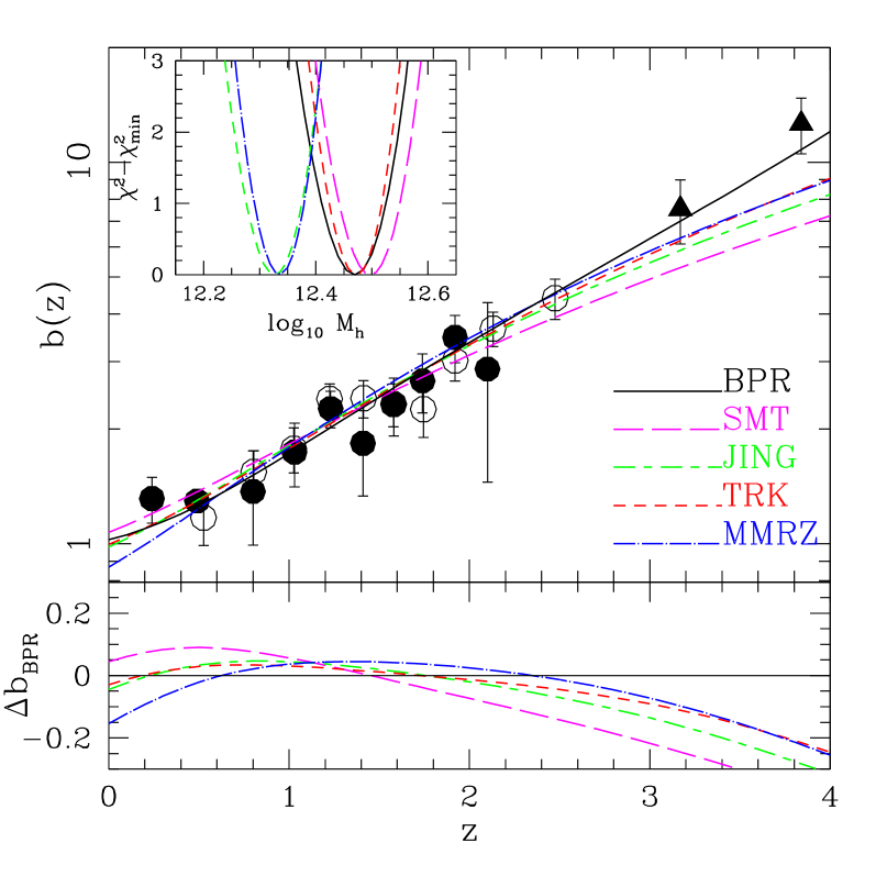
Figure 1: Main Panel: Comparison of the QSO bias data (open circles correspond to Croom et. al. 2005; filled circles to Ross et al. 2009 and filled triangles to the high redshift data of Shen et. al. 2010), with the one free parameter bias model fits (BPR: black continuous line; SMT: magenta dashed line; JING: green long-short dashed line; TRK: red short-dashed line; MMRZ: blue dot-dashed line). Lower Panel: The relative difference between the BPR model and all the rest, $\Delta b_{\rm BPR}(z)$. Inset Panel: The value of $\chi^{2}-\chi^{2}_{\rm min}$ as a function of halo mass, $M_{h}$, for the indicated bias models.

4.1.1 One free parameter models

In Table 1 we present the best fit model parameters based on the $\chi^{2}$ minimization procedure, with the first and second columns listing the fitted halo mass, $M_{h}$, derived using eq.(17) and the value of bias at $z=0$, respectively. We also present the goodness of fit statistics, as discussed previously (reduced $\chi^{2}$ and AIC_c). In the main panel of Figure $1$ we present the bias evolution models (different lines), using the best fit parameter values listed in Table 1 together with the WMAP7-scaled optical QSO bias data. The inset panel of Fig.(1) shows that the resulting $M_{h}$ values cluster around two, relatively similar, values: $\sim 3\times 10^{12}h^{-1}M_{\odot}$ and $\sim 2\times 10^{12}h^{-1}M_{\odot}$. In the lower panel we present the relative difference between the BPR model and all the rest, ie., $\Delta b_{\rm BPR}(z)=[b_{i}(z)-b_{\rm BPR}(z)]/b_{\rm BPR}(z)$.

Some basic conclusions that become evident, inspecting also Table 1, are:

• Although all one free parameter bias models appear to fit at a statistically acceptable level the optical QSO bias data, by far the best model is the BPR, which is the only model fitting also the highest redshifts ($z\raise-2.0pt\hbox{\hbox to0.0pt{\hbox{$\sim$}\hss}\raise 5.0pt\hbox{$>$}\ }3$). The MMRZ is the only model that does not fit the lowest redshifts ($z\raise-2.0pt\hbox{\hbox to0.0pt{\hbox{$\sim$}\hss}\raise 5.0pt\hbox{$<$}\ }0.3$), providing an anti-biased value at the current epoch, $b(0)=0.87$.

• The relative bias difference of the various fitted models with respect to that of BPR, $\Delta b_{\rm BPR}(z)$, indicates that the BPR, JING and TRK models have a very similar redshift dependence for $z\raise-2.0pt\hbox{\hbox to0.0pt{\hbox{$\sim$}\hss}\raise 5.0pt\hbox{$<$}\ }2.2$ (with $|\Delta b_{\rm BPR}(z)|\raise-2.0pt\hbox{\hbox to0.0pt{\hbox{$\sim$}\hss}\raise 5.0pt\hbox{$<$}\ }0.05$), while all the models show very large such deviations for $z\raise-2.0pt\hbox{\hbox to0.0pt{\hbox{$\sim$}\hss}\raise 5.0pt\hbox{$>$}\ }2.8$, reaching $|\Delta b_{\rm BPR}|\raise-2.0pt\hbox{\hbox to0.0pt{\hbox{$\sim$}\hss}\raise 5.0pt\hbox{$>$}\ }0.3$ at the largest redshifts. The SMT and MMRZ models show large deviations at the lowest redshifts as well.

• Beyond the fact that the BPR model provides by far the best fit to the QSO bias data, the second best model is the TRK model, with $\Delta$AIC${}_{c}\sim-2.9$. Furthermore, one can distinguish that the model pairs (JING, TRK) and (JING, MMRZ) are statistically equivalent ($\Delta$AIC${}_{c}\raise-2.0pt\hbox{\hbox to0.0pt{\hbox{$\sim$}\hss}\raise 5.0pt\hbox{$<$}\ }2$).

• The traditional SMT and the recently proposed MMRZ models rate the worst among all the other one parameter models, but interestingly the former provides consistent values of $M_{h}$ and $b(0)$ with those of the BPR model.

We attempt now to provide a robust average value of the DM halo mass that hosts optical QSO, using an inverse-AIC_c weighting of the different one parameter model results. This procedure provides a weighted mean and combined weighted standard deviation of the DM halo mass of:

$$(\mu_{M_{h}},\sigma_{M_{h}})=(2.72,0.56)\times 10^{12}h^{-1}M_{\odot}$$

while the weighted scatter of the mean is $\sim 0.44\times 10^{12}h^{-1}M_{\odot}$.

Finally, we point out that since it appears that mainly the 2 high-$z$ bias points are the ones that give the advantage to the BPR model with respect to the others, we perform a more conservative comparison among the models by excluding these two high-$z$ data points. We find that although the resulting halo mass and $b(0)$ are very similar to those of Table 1, with variations of a few percent, there are now three models that perform equivalently well, the BPR, JING and TRK with AIC${}_{c}\simeq 13$. The other two models perform moderately (SMT) or significantly (MMRZ) worse, as was the case also in the full data comparison, with $\Delta$AIC${}_{c}\simeq 2$ and 4, respectively.

4.1.2 Two free parameter models

We now allow a second parameter to be fitted simultaneously with the DM halo mass. Since the free parameters of the bias models have been determined using N-body simulations, it would be interesting to investigate if their simulation-based value can be reproduced by real observational data. The second free parameter that we will use is $\alpha_{1}$, $A$, $a$, $y$ and $\alpha$ for the BPR-I, BPR-II, SMT-I, TRK-I and MMRZ-I models, respectively. Note that in the case of the BPR-II model we will use the simulation based value of $\alpha_{1}$, with the free parameter $A$ being the halo-merging parameter of the BPR model (defined in section 3.5).

Model	$10^{12}h^{-1}M_{\odot}$	2ndparam.	$b(0)$	$\chi^{2}_{\rm min}/df$	AICc
BPR-I	$2.2\pm 0.4$	$4.64\pm 0.07$	1.08	$11.95/20$	$16.16$
BPR-II	$2.8\pm 0.6$	$0.008\pm 0.005$	1.02	$12.45/20$	$16.66$
SMT-I	$27.0\pm 4.0$	$0.40\pm 0.02$	0.95	$18.72/20$	$22.93$
TRK-I	$0.4\pm 0.1$	$6.14\pm 0.43$	1.11	$13.37/20$	$17.58$
MMRZ-I	$0.3\pm 0.1$	$1.21\pm 0.04$	0.87	$21.27/20$	$25.48$

Table 2: Results of the $\chi^{2}$ minimization procedure between the optical QSO data and the bias models with 2 free parameters.

Table 2 presents the best fit model parameters resulting from the $\chi^{2}$ minimization procedure, with the first and second columns representing respectively the resulting halo mass, $M_{h}$, and the second free parameter, while the third column the value of the bias at $z=0$. In Figure 2 we compare the resulting bias evolution models with the WMAP7 scaled QSO bias data (as in Figure 1), while in the lower panel we present the relative difference between the BPR-II model and all the rest, ie., $\Delta b_{\rm BPR-II}(z)=[b_{i}(z)-b_{\rm BPR-II}(z)]/b_{\rm BPR-II}(z)$.

Below we list the main conclusions of the above fitting procedure:

• A first important result is that the only model that reproduces the simulation-based second free parameter value, is the BPR-I model. The simulation based value is $\alpha_{1}=4.53$ while the fitted value, based on the QSO bias data, is $\alpha_{1}=4.64\pm 0.07$. This fact will allow us to derive the dependence of the parameters of the BPR bias evolution model on the relevant cosmological parameters (see Appendix A2).

• Fitting the BPR-II model to the QSO data provides $A=0.008\pm 0.005$ which is almost identical to the simulation determined value, used in the BPR case ($A=0.006$). As it is therefore expected, the fitted values of $M_{h}$ and $b(0)$ are almost identical to those of the one parameter BPR model, but the statistical significance of the BPR-II model is lower than that of the BPR due to its 2 free parameters.

• Although the SMT-I and TRK-I models appear now to fit slightly better the QSO bias data, especially the higher $z$ range, this happens on the expense of providing unexpected values for the $M_{h}$ and very different values of the second fitted parameter with respect to their simulation based value. For example, the SMT-I model provides a huge halo mass, $\sim$9 times larger than that provided by the corresponding one parameter model. This should be attributed to the fact that the fitted second parameter, $a$, is significantly smaller than the nominal value of 0.707. Similarly, the TRK-I model provides a very small value of $M_{h}$, a factor of $\sim 9$ less than of the corresponding one parameter model, while the resulting value $y=6.14$ implies that $\Delta\simeq 10^{6}$, a value extremely large and unphysical. Finally, the MMRZ-I model provides again a very small value of $M_{h}$, while it is the only two-parameter model that fits the data worst than the corresponding one parameter model. This is due to the fact that we have used $\kappa=0.44$ and not $\kappa=0.23$, which is used in the one free parameter model, as suggested by MMRZ. Had we used the latter $\kappa$ value we would have found an extremely small value of $M_{h}\simeq 10^{10}h^{-1}M_{\odot}$. These results probably indicate a degeneracy between the two fitted parameters, a fact which we indeed confirm for the SMT-I, TRK-I and MMRZ-I models, as can be seen in Figure 3 where we plot the 1, 2 and 3$\sigma$ likelihood contours in the parameter solution plane. Contrary to the above models, no such degeneracy is present for BPR-I model. Note that in Fig.3 the cross indicates the best 2-parameter solution, while the dashed line indicates the simulation based value of the second parameter. In the case of the TRK-I model the latter corresponds to the virialization value ($y=\log_{10}355$), used in the one free parameter fit.

  

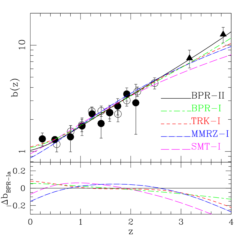
  Figure 2: Comparison of the QSO bias data with the two free parameter bias models (their line types and colors are indicated in the Figure). Lower Panel: The relative difference, $\Delta b_{\rm BPR-II}(z)$, between the BPR-II and the rest of the models.

• Beyond the previously mentioned fundamental flow of the two parameter models (SMT-I, TRK-I and MMRZ-I), they all provide relatively comparable to the BPR-II model fits of the QSO bias data but only within the range $0.8\raise-2.0pt\hbox{\hbox to0.0pt{\hbox{$\sim$}\hss}\raise 5.0pt\hbox{$<$}\ }z\raise-2.0pt\hbox{\hbox to0.0pt{\hbox{$\sim$}\hss}\raise 5.0pt\hbox{$<$}\ }2.4$ (see lower panel of Fig.2). Furthermore, the MMRZ-I model, as in the case of the one free parameter fit, provides an anti-biased value at $z\raise-2.0pt\hbox{\hbox to0.0pt{\hbox{$\sim$}\hss}\raise 5.0pt\hbox{$<$}\ }0.2$, while it also provides the worst overall fit to the QSO bias data.

• Finally, the BPR one parameter model scores the best among all the one or two free parameter models and over the whole available QSO bias redshift range, while it is statistically equivalent with the BPR-I and BPR-II models (since $|\Delta$AIC${}_{c}|\raise-2.0pt\hbox{\hbox to0.0pt{\hbox{$\sim$}\hss}\raise 5.0pt\hbox{$<$}\ }1.8$; see Table 3).

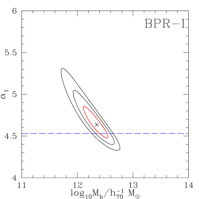
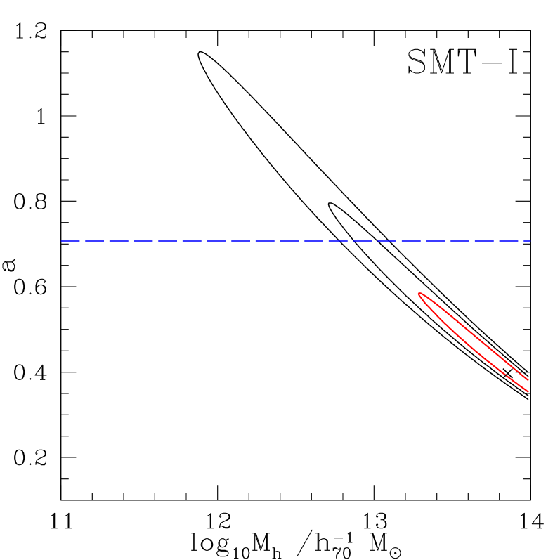
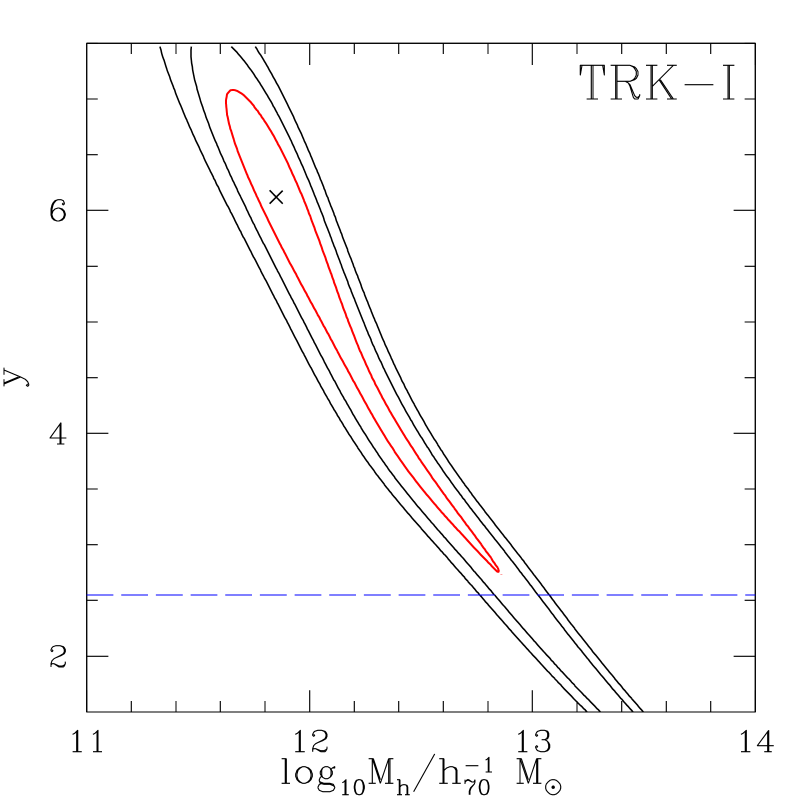
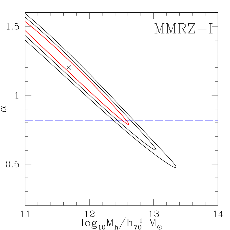
Figure 3: Contour plots of the two fitted parameter solution space. The 1$\sigma$ level is indicated by the relatively thicker red curve. The blue dashed line indicates the simulation based value of the y-axis parameter.

We assess in a more quantitative manner the statistical relevance of the different theoretical bias models in representing the observational QSO bias data by using the information theory parameter AIC_c and presenting in Table 3 the model pair difference $\Delta$AIC_c. As previously discussed a smaller AIC_c value indicates a model that better fits the data, while a small $|\Delta$AIC${}_{c}|$ value (ie., $\raise-2.0pt\hbox{\hbox to0.0pt{\hbox{$\sim$}\hss}\raise 5.0pt\hbox{$<$}\ }2)$ indicates that the two comparison models represent the data at a statistically equivalent level.

	BPR-I	BPR-II	SMT	JING	TRK	MMRZ
BPR	-1.3	-1.8	-10.3	-5.1	-2.9	-7.3
BPR-I		-0.5	-9.0	-3.8	-1.6	-6.0
BPR-II			-8.5	-3.3	-1.1	-5.5
SMT				5.2	7.4	3.1
JING					2.2	-2.1
TRK						-4.3

Table 3: Results of the pair difference $\Delta$AIC_c for the bias evolution models fitted to the optical QSO data.

Due to the resulting unphysical second free parameter, as discussed previously, we do not use in Table 3 a comparison based on the SMT-I, TRK-I and MMRZ-I models. It is obvious that the one free parameter BPR model fairs the best among any model, while it is statistically equivalent, as indicated by the relevant values of $\Delta$AIC_c, to the BPR-I and BPR-II models and to a slightly lesser degree to the TRK model.

4.2 Optical VVTS galaxy Results

This model-data comparison takes place at relatively low redshifts ($z<1.5$), covering a small dynamical range in $z$, and therefore we will use only the one free parameter models to fit the galaxy bias data. An additional reason is that even with the much larger $z$-dynamical range covered by the QSO data, the second parameter could not be constrained (except for the case of the BPR-I and BPR-II models).

The results of the $\chi^{2}$-minimization procedure are presented in Table 4, while in Figure 4 we present the model fits to the galaxy bias data. Note that the layout of Figure 4 is as Figure 1.

Model	$10^{11}h^{-1}M_{\odot}$	$b(0)$	$\chi^{2}_{min}/df$	AICc
BPR	$6.0\pm 2.5$	0.99	$0.29/4$	2.29
SMT	$6.4\pm 1.9$	0.90	$0.45/4$	2.45
JING	$5.1\pm 1.3$	0.83	$0.93/4$	2.93
TRK	$7.8\pm 1.9$	0.86	$0.74/4$	2.74
MMRZ	$6.1\pm 1.3$	0.70	$2.10/4$	4.10

Table 4: Results of the $\chi^{2}$ minimization procedure between the one free parameter models and the optical VVTS galaxy bias data.

It is evident that the BPR model fairs the best providing the lowest reduced $\chi^{2}$ and AIC_c parameter with respect to the other models, while the MMRZ model fairs the worst. However, due to the small dynamical range in redshift, the information theory pair model characterization parameter, $\Delta$AIC_c, indicates that all the bias models are statistically equivalent in representing the bias data, since $\Delta$AIC${}_{c}\raise-2.0pt\hbox{\hbox to0.0pt{\hbox{$\sim$}\hss}\raise 5.0pt\hbox{$<$}\ }1.8$ for any model pair. As in the QSO case, we provide an average halo mass that hosts VVTS optical galaxies using an AIC_c weighted procedure over the different one-parameter bias models. The resulting weighted mean and combined weighted standard deviation are:

$$(\mu_{M_{h}},\sigma_{M_{h}})=(6.3,2.1)\times 10^{11}h^{-1}M_{\odot}$$

while the weighted scatter of the mean is also $\sim 0.9\times 10^{11}h^{-1}M_{\odot}$.

It is interesting to point out that the only model that finds that at $z=0$ the optical galaxies are unbiased ($b_{0}\simeq 1$), in agreement with other studies of wide-area optical galaxy catalogues (Verde et al. 2002; Lahav et al. 2002), is the BPR model, while all the other models indicate that optical galaxies are quite anti-biased with $b(0)\leq 0.9$.

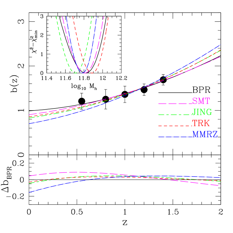
Figure 4: Results of the $\chi^{2}$ minimization procedure between the VVTS galaxy bias data and the bias models with one free parameter.

5 Conclusions

In this work we assess the ability of five recent bias evolution models to represent a variety of observational bias data, based either on optical QSO or optical galaxies. To this end we applied a $\chi^{2}$ minimization procedure between the observational bias data, after rescaling them to the WMAP7 cosmology, with the model expectations, through which we fit the model free parameters.

In performing this comparison we assume that each halo is populated by one extragalactic mass tracer, being a QSO or a galaxy; an assumption which is justified since the observational data have been estimated on the basis of either the large-scale clustering ($>1h^{-1}$ Mpc), corresponding to the halo-halo term, or the corrected for non-linear effects variance of the smoothed (on 8 $h^{-1}$ Mpc scales) density field.

The comparison shows that all models fit at an acceptable level the QSO data as indicated by the their reduced $\chi^{2}$ values. Using the information theory characteristic, AIC_c, which takes into account the different number of model free parameters we find that the model that rates the best among all the other is the Basilakos & Plionis (2001; 2003) model with the tracer merging extension of Basilakos, Plionis & Ragone-Figueroa (2008), which is the only model fitting accurately the optical QSO bias data over the whole redshift range traced ($0<z<4$). The only other model that is statistically equivalent at an acceptable level is that of Tinker et al. (2010). The average, over the different bias models, DM halo mass that hosts optical QSOs is: $M_{h}\simeq 2.7(\pm 0.6)\times 10^{12}h^{-1}M_{\odot}$.

Finally, all the investigated bias models fit well and at a statistically equivalent level the VVTS galaxy bias data, with the BPR model scoring again the best, and the MMRZ the worst. The average, over the different bias models, DM halo mass hosting optical galaxies is: $M_{h}\simeq 6(\pm 2)\times 10^{11}h^{-1}M_{\odot}$.

Appendix A Simulation based BPR model Parameter estimation

A.1 $\Lambda$CDM Simulations

We have run a new WMAP7 $\Lambda$CDM N-body simulation using the GADGET-2 code (Springel 2005) with dark matter only. The size of the box simulation is $500h^{-1}$ Mpc and the number of particles is $512^{3}$. The adopted cosmological parameters are the following: $\Omega_{m}=0.273$ $\Omega_{\Lambda}=0.727$, $h=0.704$, $\sigma_{8}=0.81$ and the particle mass is $7.07\times 10^{10}h^{-1}M_{\odot}$, comparable to the mass of a single galaxy. The initial conditions were generated using the GRAFIC2 package (Bertschinger 2001). We also use a similar size simulation, generated in Ragone-Figueroa & Plionis (2007), of a $\Lambda$CDM model with $\Omega_{\rm m}=0.3$, $\Omega_{\Lambda}=0.7$, $h=0.72$ and $\sigma_{8}=0.9$.

The dark matter haloes were defined using a FoF algorithm with a linking length $l=0.17\langle n\rangle^{-1/3}$, where $\langle n\rangle$ is the mean particle density.

We estimate the bias redshift evolution of the different DM haloes, with respect to the underlying matter distribution, by measuring their relative fluctuations in spheres of radius 8 $h^{-1}$ Mpc, according to the definition of eq.(3), ie.,

$$b(M,z)=\frac{\sigma_{8,h}(M,z)}{\sigma_{8,m}(z)}\;,$$ (32)

where the subscripts $h$ and $m$ denote haloes and the underlying mass, respectively. The values of $\sigma_{8,h}(M,z)$, for haloes of mass $M$, are computed at different redshifts, $z$, by:

$$\sigma^{2}_{8,h}(M,z)=\left\langle\left(\frac{N-\bar{N}}{\bar{N}}\right)^{2}\right\rangle-\frac{1}{\bar{N}}\;,$$ (33)

where $\bar{N}$ is the mean number of such haloes in spheres of 8 $h^{-1}$ Mpc radius and the factor $1/\bar{N}$ is the expected Poissonian contribution to the value of $\sigma^{2}_{8,h}$. Similarly, we estimate at each redshift the value of the underlying mass $\sigma_{8,m}$. In order to numerically estimate $\sigma^{2}_{8,j}$ we randomly place $N_{\rm rand}$ sphere centers in the simulation volume, such that the sum of their volumes is equal to $\sim 1/8$ the simulation volume ($N_{\rm rand}=8000$). This is to ensure that we are not oversampling the available volume, in which case we would have been multiply sampling the same halo or mass fluctuations. The relevant uncertainties are estimated as the dispersion of $\sigma^{2}_{8,j}$ over 20 bootstrap re-samplings of the corresponding halo sample.

Figure 5: The Parameters ${\cal C}_{1}$ and ${\cal C}_{2}$ derived from the WMAP7 (filled points) and WMAP1 (open points) $\Lambda$CDM simulation (points). Continuous lines correspond to the function form of eq. (A3), with best fit parameters shown in Table A1.

Model	$\alpha_{1}$	$\alpha_{2}$	$\beta_{1}$	$\beta_{2}$
WMAP1	3.30$\pm 0.13$	-0.36$\pm 0.01$	0.34$\pm 0.04$	0.32$\pm 0.04$
WMAP7	4.53$\pm 0.22$	-0.41$\pm 0.02$	0.37$\pm 0.04$	0.36$\pm 0.04$

Table 5: Results of the $\chi^{2}$ minimization used to evaluate the parameters that enter in the ${\cal C}_{1}$ and ${\cal C}_{2}$ constants (which depend on DM halo mass) of the BPR bias evolution model.

Note that we do not explicitely correct for possible non-linear effects in $\delta$ (although the density field is indeed smoothed on linear scales - 8 $h^{-1}$ Mpc); we do however expect that such effects should be mostly cancelled in the overdensity ratio definition of the bias.

We use the DM halo bias evolution, measured in the two simulations, for different DM halo mass range subsamples in order to constrain the constants of our bias evolution model, ie., ${\cal C}_{1},{\cal C}_{2}$. The procedure used is based on a $\chi^{2}$ minimization of whose details are presented in BPR and thus will not be repeated here. In Fig.A1 we present as points the simulations based values of these parameters, for both cosmologies used, and as continuous curves their analytic fits, which are given in eqs.(20) and (21). The resulting values of the parameters $\alpha_{1,2}$ and $\beta_{1,2}$ can be found in Table A1. It is interesting to note that the slope of the functions ${\cal C}_{1}$ and ${\cal C}_{2}$ is roughly a constant and independent of cosmology, with a value $\beta_{1}\simeq\beta_{2}\simeq 0.35(\pm 0.06)$.

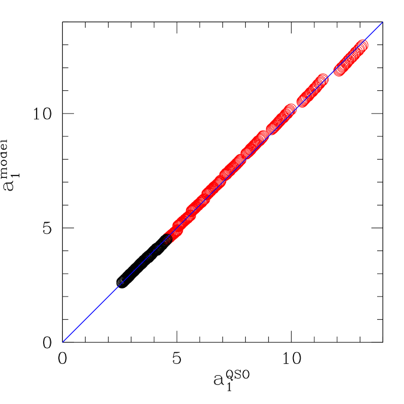
Figure 6: Correlation between (a) the best fitted $\alpha_{1}$ values of the BPR model using the QSO bias data scaled to different cosmologies for a grid of $\Omega_{m}$ and $\sigma_{8}$ values and (b) the predicted $\alpha_{1}$ values, based on eq.(35). The red points correspond to $\Omega_{m}\leq 0.273$ while the black points to $\Omega_{m}>0.273$.

A.2 Dependence of the BPR model constants on Cosmology

The dependence of the constants $\alpha_{1}$ and $\alpha_{2}$ of the BPR bias model on the different cosmological parameters is an important prerequisite for the versatile use of the model in investigating the bias evolution of different mass tracers and determine the mass of the dark matter halos which they inhabit. In Basilakos & Plionis (2001) we predicted a power law dependence of $\alpha_{2}$ on $\Omega_{m}$. Indeed, fitting such a dependence, using the WMAP1 and WMAP7 $\Lambda$CDM simulations, we find:

$$\alpha_{2}(\Omega_{m})=-0.41\left(\frac{0.273}{\Omega_{m}}\right)^{n}\;\;{\rm with}\;\;n\simeq 2.8/2$$ (34)

consistent with the value $n=3/2$ anticipated in Basilakos & Plionis (2001).

Now, in order to investigate the dependence on different cosmological parameters of the parameter $a_{1}$, we have used the optical QSO data and the procedure outlined in section 2.2 to scale the QSO bias data to different flat cosmologies, using a grid of $\Omega_{m}$ and $\sigma_{8}$ values. The grid was defined as follows: $\Omega_{m}\in[0.18,0.5]$ and $\sigma_{8}\in[0.7,0.94]$, both in steps of 0.01. We then minimize the BPR bias evolution model to the scaled bias data to different cosmologies QSO, finally providing for each pair of ($\Omega_{m},\sigma_{8}$) values the best fitted $\alpha_{1}$ and $M_{h}$ values.

Then using a trial and error approach to select the best functional dependence of the derived $\alpha_{1}(\Omega_{m},\sigma_{8})$ values to the relevant cosmological parameters, we find a best fit model of the form:

$$\alpha_{1}(\Omega_{m},\sigma_{8})\simeq 4.53\left(\frac{0.81}{\sigma_{8}}\right)^{\kappa_{1}}\exp{\left[\kappa_{2}(\Omega_{m}-0.273)\right]}$$$$ (35)

with

$$(\kappa_{1},\kappa_{2})=\left\{\begin{array}[]{ll}(12.15,0.30)&\Omega_{m}\leq 0.273\\ (8.70,0.37)&\Omega_{m}>0.273\end{array}\right.$$ (36)

In Fig. A2 we correlate the derived $\alpha_{1}(\Omega_{m},\sigma_{8})$ values, resulting from fitting the BPR bias evolution model to the scaled QSO bias data, to those predicted by the model of eq.(35). It is evident that the correspondence is excellent, indicating that indeed the above estimated cosmological dependence of $\alpha_{1}$ is the indicated one.

References

- [1] Akaike, H., 1974, IEEE Transactions of Automatic Control, 19, 716
- [2] Bagla J. S., 1998, MNRAS, 299, 417
- [3] Bardeen, J. M., Bond, J. R., Kaiser, N., Szalay, A. S., 1986, ApJ, 304, 15
- [4] Basilakos, S., Plionis, M., 2001, ApJ, 550, 522
- [5] Basilakos, S., Plionis, M., 2003, ApJ, 593, L61
- [6] Basilakos, S., Plionis, M., Figueroa, C. R., 2008, ApJ, 678, 627
- [7] Basilakos, S., Plionis, M., Pouri, A., 2011, PhRvD, 83, 123525
- [8] Bertschinger, E., 2001, ApJS, 137, 1
- [9] Cole, S., Kaiser, N., 1989, MNRAS, 237, 1127
- [10] Cole, S., Coles, P., Matarrese, S., Moscardini, L., 1994, MNRAS, 268, 966
- [11] Croom, S. M., et. al., 2005, MNRAS, 356, 415
- [12] Davis, M., Peebles, P. J. E, 1983, ApJ, 267, 465
- [13] Davis, T.M. et al., 2007, ApJ, 666, 716
- [14] de Simon, A., Maggiore, M., Riotto, A., 2011, MNRAS, 412, 2587
- [15] Fry, J. N., 1996, ApJ, 461, L65
- [16] Godlowski, W., Szydlowski, M., 2005, Phys.Lett.B, 540, 1
- [17] Eisenstein, D. J., Hu, W., 1998, ApJ, 496, 605
- [18] Hamana, T., Yoshira, N., Suto, Y., 2002, ApJ, 568, 455
- [19] Hamilton, A.J.S., 1992, ApJ, 385, L5
- [20] Hamilton, A.J.S., 1998, ASSL, 231, 185 astro-ph/9708102
- [21] Hui L., Parfrey K. P., 2008, Phys.Rev.D, 77, 043527
- [22] Jing, Y. P., 1998, ApJ, 503, L9
- [23] Kaiser, N., 1984, ApJ, 284, L9
- [24] Kaiser, N., 1987, MNRAS, 227, 1
- [25] Komatsu, E., et al., 2011, ApJS, 192, 18
- [26] Lahav, O., et al., 2002, MNRAS, 333, 961
- [27] Liddle, A.R., 2004, MNRAS, 351, L49
- [28] Linder, E. V., 2005, Phys. Rev. D., 72, 043529
- [29] Ma, C-P., Maggiore, M., Riotto, A., Jun, Z., 2011, MNRAS, 411, 2644
- [30] Maggiore, M., Riotto, A., 2010, ApJ, 711, 907
- [31] Manera, M., Sheth, R.K., Scoccimarro, R., 2009, MNRAS, 402, 589
- [32] Manera, M., Gaztanaga, E., 2011,
- [33] Marinoni, C., et. al., 2005, A&A, 442, 801
- [34] Matarrese, S., Coles, P., Lucchin, F., Moscardini, L., 1997, MNRAS, 286, 115
- [35] Mo, H. J., White, S. D. M., 1996, MNRAS, 282, 347
- [36] Mo, H. J., Jing, Y. P., White, S. D. M., 1997, MNRAS, 284, 189
- [37] Moscardini, L., Coles, P., Lucchin, F., Matarrese, S., 1998, MNRAS, 299, 95
- [38] Myers, A. D., et. al., 2006, ApJ, 658, 85
- [39] Nusser, A., Davis, M., 1994, ApJ, 421, L1
- [40] Pillepich A., Porciani C., Han O., 2010, MNRAS, 402, 191
- [41] Press, W. H., Schechter, P., 1974, ApJ, 187, 425
- [42] Ragone-Figueroa, C., & Plionis, M. 2007, MNRAS, 377, 1785
- [43] Ross, N. P., et. al., 2009, ApJ, 697, 1634
- [44] Saini, T.D., Weller, J., Bridle, S.L., 2004, MNRAS, 348, 603
- [45] Schaefer B. M., Douspis M., Aghanim N., 2009, MNRAS, 397, 925
- [46] Seljak, U., Warren, M. S., 2004, MNRAS, 355, 129
- [47] Shen, Y.,et. al., 2009, ApJ, 697, 1656
- [48] Sheth, R. K., Tormen, G., 1999, MNRAS, 308, 119
- [49] Sheth, R. K., Mo, H. J., Tormen, G., 2001, MNRAS, 323, 1
- [50] Simon P., A&A, 2005, 430, 827
- [51] Springel, V. 2005, MNRAS, 364, 1105
- [52] Sugiura, N. 1978, Communications in Statistics A, Theory & Methods, 7, 13
- [53] Sugiyama, N., 1995, ApJS, 100, 281
- [54] Tegmark, M., Peebles, P. J. E., 1998, ApJ, 500, L79
- [55] Tinker, J. L., Weinberg, D. H., Zheng, Z., 2005, ApJ, 631, 41
- [56] Tinker, J. L., et. al. 2010, ApJ, 724, 878
- [57] Valageas P., 2009, A&A, 508, 93
- [58] Valageas P., 2011, A&A, 525, 98
- [59] Verde L., et al., 2002, MNRAS, 335, 432
- [60] Wang, L., Steinhardt, J. P., 1998, ApJ, 508, 483
- [61] Weinberg, N.N. & Kamionkowski, M., 2003, MNRAS, 341, 251