Resonant Adiabatic Passage with Three Qubits

Abstract

We investigate the non-adiabatic implementation of an adiabatic quantum teleportation protocol, finding that perfect fidelity can be achieved through resonance. We clarify the physical mechanisms of teleportation, for three qubits, by mapping their dynamics onto two parallel and mutually-coherent adiabatic passage channels. By transforming into the adiabatic frame, we explain the resonance by analogy with the magnetic resonance of a spin-1/2 particle. Our results establish a fast and robust method for transferring quantum states, and suggest an alternative route toward high precision quantum gates.

Fault-tolerant quantum computation requires high-precision quantum gates with noise thresholds between $10^{-4}$ and $10^{-2}$, depending on the fault-tolerance scheme Shor ; Preskill . This stringent requirement poses significant technical challenges, even for the more mature qubit architectures, such as those based on trapped ions Lanyon_Science11 . Identifying gate protocols that are both fast and robust is therefore an important research objective for quantum information processing.

One potential approach to robust quantum gates is based on the adiabatic principle – a fundamental tenet of quantum mechanics Messiah . According to the adiabatic theorem, a quantum system in an eigenstate remains there, provided that the Hamiltonian varies slowly in time. Applications of the adiabatic theorem include the Born-Oppenheimer approximation and the Landau-Zener-Stückelberg transition at an avoided crossing, the latter having been demonstrated in both superconducting and spin qubits Oliver ; Gaudreau12 . Other experimental implementations include adiabatic population transfers between two or three-level systems, known as adiabatic passages (AP) Oreg84 ; Bergmann98 ; Kral07 ; Shore08 , which have been demonstrated in atomic, molecular, and optical devices. There are also theoretical proposals for realizing AP with superconducting qubits Norigroup and quantum dot arrays Greentree04 . Adiabatic quantum information processing Farhi01 entails the adiabatic transformation of the ground state of an initial Hamiltonian into that of a target Hamiltonian. Compared to the quantum circuit model, adiabatic gates are resistant to decoherence when a finite excitation gap persists throughout the evolution, and they are robust to gating errors, by virtue of adiabaticity. This can be a drawback however, since the maximum speed of an adiabatic gate is also proportional to the spectral gap.

In this Letter we investigate a non-adiabatic form of adiabatic quantum teleportation (AQT). Conventional AQT was proposed in the context of fault tolerant quantum computation Bacon09 . Here, we focus on systems with three qubits, where we can solve the evolution analytically. We show that resonances occur, enabling teleportation that is fast, fault-tolerant, and potentially perfect. This surprising effect can be explained in the language of spin resonance, by transforming into the adiabatic frame. Our results point toward a new paradigm for quantum algorithms, based on fast adiabatic gates. Our work also provides an interesting mapping between three coupled qubits and a three-level atom, which could lead to further spin analogies from atomic $\Lambda$-system physics. The experimental requirements for implementing AQT have already been demonstrated in the laboratory for triple quantum dots Gaudreau12 and superconducting circuits Martinis11 . Our results could therefore be tested immediately.

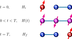
Figure 1: (color online). The couplings and the information distribution (by color and arrow) among three qubits are shown at the initial, intermediate, and final stages of adiabatic quantum teleportation.

The adiabatic quantum teleportation protocol is illustrated in Fig. 1. Initially, qubit 1 is isolated and prepared in an arbitrary superposed state, while qubits 2 and 3 are coupled, as described below, and prepared in the maximally entangled singlet state. The antiferromagnetic coupling between qubits 1 and 2 (2 and 3) is then turned on (off) slowly. When the evolution is complete, the quantum state of qubit 1 will be teleported to qubit 3. As proposed in Ref. Bacon09 , the scheme succeeds when the run time $T$ satisfies the adiabatic theorem.

To explore non-adiabatic effects, we solve the exact dynamics of the three-qubit system. It is governed by a time-dependent Hamiltonian, which smoothly changes from the initial Hamiltonian $H_{i}$ at $t=0$ to the final Hamiltonian $H_{f}$ at $t=T$:

$$H(t)=f(t)\,H_{i}+g(t)\,H_{f}\,.$$ (1)

The initial and final Hamiltonians are given by

$$H_{i} =J\left(\,\sigma_{2x}\,\sigma_{3x}+\sigma_{2y}\,\sigma_{3y}+\gamma\,\sigma_{2z}\,\sigma_{3z}\,\right)\,,$$ (2a)

$$H_{f} =J\left(\,\sigma_{1x}\,\sigma_{2x}+\sigma_{1y}\,\sigma_{2y}+\gamma\,\sigma_{1z}\,\sigma_{2z}\,\right)\,,$$ (2b)

where $\sigma_{i\mu}$ are the Pauli operators with $i=1,2,3$ and $\mu=x,y,z$, and $J$ is the strength of the qubit-qubit coupling. The anisotropy parameter $\gamma=0$ corresponds to an XX coupling, available in superconducting qubits, while $\gamma=1$ corresponds to the isotropic Heisenberg coupling of spin qubits. The interpolation or switching functions $f(t)$ and $g(t)$ satisfy $f(0)=g(T)=1$ and $f(T)=g(0)=0$. Here we consider two ways to connect $H_{i}$ to $H_{f}$: (i) a linear interpolation with $f(t)=1-t/T$ and $g(t)=t/T$, and (ii) a harmonic interpolation with $f(t)=\cos({\pi t}/{2T})$ and $g(t)=\sin({\pi t}/{2T})$.

AQT begins with an initial three-qubit state given by

$$|{\psi(0)}\rangle=\bigl{(}a|{0}\rangle+b|{1}\rangle\bigr{)}_{1}\otimes\frac{1}{\sqrt{2}}\bigl{(}|{01}\rangle-|{10}\rangle\bigr{)}_{2,3}\,,$$ (3)

where $a|{0}\rangle+b|{1}\rangle$ is the arbitrary state to be teleported. The success of AQT is measured by the fidelity $F(T)=|\langle{\psi_{T}}|{\psi(T)}\rangle|^{2}$ where $|{\psi(T)}\rangle$ is the final state at time $T$ and $|{\psi_{T}}\rangle=\frac{1}{\sqrt{2}}\bigl{(}|{01}\rangle-|{10}\rangle\bigr{)}_{1,2}\otimes\bigl{(}a|{0}\rangle+b|{1}\rangle\bigr{)}_{3}$ is the target state. The dynamics of AQT is governed by the time-dependent Hamiltonian (1), with the initial state (3).

Hamiltonian (1) satisfies the commutation relation $[H(t),S_{z}]=0$, so that the $z$-component of the total spin angular momentum $S_{z}\equiv\frac{1}{2}\left(\sigma_{1z}+\sigma_{2z}+\sigma_{3z}\right)$ is a good quantum number, which is conserved during evolution. The three-qubit Hamiltonian (1) is thus block-diagonal:

$$H(t)=\underbrace{H_{3}}_{\rm up}\oplus\underbrace{H_{3}}_{\rm down}\oplus H_{1}\oplus H_{1}\,.$$ (4)

The two $H_{1}$ operators act on $|{000}\rangle$ and $|{111}\rangle$, while the two $H_{3}$ operators act on the distinct subspaces ${\cal H}_{1/2}=\text{Span}(|{100}\rangle,|{010}\rangle,|{001}\rangle)$ and ${\cal H}_{-1/2}=\text{Span}(|{011}\rangle,|{101}\rangle,|{110}\rangle)$, and have the same form

$$H_{3}(t)=J\begin{bmatrix}(f-g)\gamma&2g&0\\ 2g&-(f+g)\gamma&2f\\ 0&2f&-(f-g)\gamma\end{bmatrix}\,.$$ (5)

Interestingly, $H_{3}$ is also the AP Hamiltonian for a 3-level atom Bergmann98 ; Kral07 ; Shore08 , with the switching functions $f(t)$ and $g(t)$ being the Stokes and pump pulses in the context of AP. For the initial states we consider, the $H_{1}$ operators are never involved in the system evolution. The AQT protocol therefore consists of two parallel, identical and mutually-coherent APs governed by $H_{3}$, corresponding to the $S_{z}=\pm\frac{1}{2}$ components of the three-qubit system.

To understand the dynamics of AQT, we solve the time-dependent Schrödinger equation with Hamiltonian (5) in two ways. First, we consider the adiabatic limit, for which there is a mapping between AQT and two mutually-coherent APs. Second, we obtain numerical solutions (and in one case, an analytical solution) for finite $T$. We also consider the separate cases of XX and Heisenberg couplings.

The adiabatic theorem states that, starting from an eigenstate $|{E_{n}(0)}\rangle$, the adiabatically evolved state $|{\psi(t)}\rangle\simeq e^{-i/\hbar\int_{0}^{t}E_{n}(t^{\prime})\,dt^{\prime}+\gamma_{B}}\,|{E_{n}(t)}\rangle\,$ is simply an instantaneous eigenstate, up to a phase factor. Here, $\gamma_{B}$ is the Berry phase, and $E_{n}$ and $|{E_{n}}\rangle$ are the instantaneous eigenvalues and eigenstates of $H_{3}(t)$, defined by

$$H_{3}(t)\,|{E_{n}(t)}\rangle=E_{n}(t)\,|{E_{n}(t)}\rangle\,.$$ (6)

Solving Eq. (6) for an XX coupling ($\gamma=0$), gives the instantaneous energy levels $E_{0}(t)=0$ and $E_{\pm}(t)=\pm 2J\sqrt{f^{2}+g^{2}}$, with the corresponding eigenstates

$$|{E_{0}(t)}\rangle =\begin{bmatrix}\cos\theta\\ 0\\ -\sin\theta\end{bmatrix}\,,\quad|{E_{\pm}(t)}\rangle=\frac{1}{\sqrt{2}}\begin{bmatrix}\sin\theta\\ \pm 1\\ \cos\theta\end{bmatrix}\,.$$ (7)

Here, the mixing angle $\theta=\tan^{-1}[g(t)/f(t)]$ runs from $0$ to $\pi/2$ as time $t$ goes from 0 to $T$. For the Heisenberg coupling ($\gamma=1$), the instantaneous energy levels are $E_{0}(t)/J=(f+g)$ and $E_{\pm}(t)/J=[-f-g\pm 2\sqrt{f^{2}-fg+g^{2}}]$, with the corresponding eigenstates

$$|{E_{0}(t)}\rangle =\frac{1}{\sqrt{3}}\begin{bmatrix}1&1&1\end{bmatrix}^{T}\,,$$ (8a)

$$|{E_{\pm}(t)}\rangle =\frac{1}{\sqrt{\cal N}}\begin{bmatrix}\sin\theta\\ -\cos\theta\pm\sqrt{1-\cos\theta\sin\theta}\\ \cos\theta-\sin\theta\mp\sqrt{1-\cos\theta\sin\theta}\end{bmatrix},$$ (8b)

where ${\cal N}\equiv 2(2\cos\theta-\sin\theta)\sqrt{q}+4q$, $q=1-\cos\theta\sin\theta$.

Equation (5) governs the evolution of both AQT and conventional AP, as depicted in Fig. 2. For AP, the population of a $\Lambda$-type system is transferred from state $|{1}\rangle$ to $|{3}\rangle$, while state $|{2}\rangle$ remains unpopulated Bergmann98 ; Kral07 ; Shore08 . Paradoxically, the AP pulse sequence appears to occur in reverse order (S followed by P), as shown in panel (a). The instantaneous eigenstate used in this evolution is $|{E_{0}(t)}\rangle$ from Eq. (7). For AQT, on the other hand, the instantaneous eigenstate used is $|{E_{-}}\rangle$ in Eqs. (7) or (8), leading to slight differences between panels (a) and (b). In panels (b) and (c), we see that the “up” state ($|{0}\rangle$) is transferred from the left-most qubit to the right-most qubit, following a similarly counter-intuitive pulse sequence. Since the $H_{3}$ operators are identical for the subspaces ${\cal H}_{1/2}$ and ${\cal H}_{-1/2}$, their separate evolutions are also identical. Thus, as illustrated in Fig. 1, an arbitrary state $a|{0}\rangle+b|{1}\rangle$ of qubit $1$ in Eq. (3) is transmitted to qubit $3$ via two mutually-coherent evolutions.

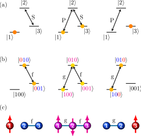
Figure 2: (color online). Adiabatic passage protocols for (a) $\Lambda$-type levels, (b) the “up” component (red $|{0}\rangle$) of a 3-qubit system, and (c) the corresponding spin configurations. From right to left: the initial, intermediate, and final stages of evolution. In (a) and (b), filled circles represent populations of levels. $S$ and $P$ stand for the Stokes and pump pulses.

The adiabatic solution described above is only valid when $JT/\hbar\gg 1$. In this limit, Eqs. (7) and (8) give a perfect (adiabatic) fidelity, $F_{\rm ad}(T)=1$. When $T$ is finite however, the adiabatic theorem predicts that $1-F\propto(JT/\hbar)^{-2}$. To obtain an infidelity $1-F<10^{-6}$, the adiabatic gate time should be $JT/\hbar\sim{\cal O}(10^{3})$, much longer than a conventional gate, for which $JT/\hbar\sim{\cal O}(1)$. Such slow adiabatic evolution could obviously cause problems, despite its intrinsic fault tolerance. However, when we perform a numerical integration of the time-dependent Schrödinger equation governed by Hamiltonian (5), we find that the infidelity $1-F$ as a function of evolution time $T$ is far from a smooth quadratic function. Instead, while it approaches the predicted upper envelope, there are also striking resonance features where the infidelity dips to zero, as shown in Fig. 3.

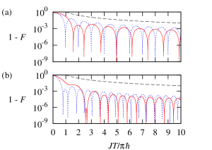
Figure 3: (color online). Infidelity $(1-F)$ is plotted as a function of $JT/\pi\hbar$ for (a) XX and (b) Heisenberg couplings, using linear and harmonic interpolation functions (solid red and dotted blue lines, respectively). The black dashed line represents $(1-F)\propto 1/(JT)^{2}$ for comparison.

The origin of the unexpected resonances in AQT fidelity becomes clear when we consider the XX coupling with harmonic interpolation functions. For this special case, we can obtain an analytical solution by transforming into the adiabatic frame Carroll , as illustrated in Fig. 4. We define

$$D(t)=A^{-1}(t)H_{3}(t)A(t)\,,\quad|{\psi(t)}\rangle=A(t)|{\phi(t)}\rangle\,,$$ (9)

where the column vectors of $A(t)$ are the instantaneous eigenstates given by Eq. (7). The Schrödinger equation in the adiabatic frame takes the form

$$i\hbar\frac{\partial}{\partial t}|{\phi(t)}\rangle =\left[D(t)-i\hbar A^{-1}(t)\frac{\partial A(t)}{\partial t}\right]|{\phi(t)}\rangle\,,$$ (10a)

$$=H_{\rm tr}|{\phi(t)}\rangle\,.$$ (10b)

For harmonic interpolation and XX couplings, the transformed Hamiltonian $H_{\rm tr}$ becomes time-independent:

$$H_{\rm tr} =2J\begin{bmatrix}-1&0&0\\ 0&0&0\\ 0&0&1\ \end{bmatrix}+\frac{\pi\hbar}{2T}\frac{1}{\sqrt{2}}\begin{bmatrix}0&i&0\\ -i&0&-i\\ 0&i&0\end{bmatrix}$$ (11a)

$$=\hbar\omega_{0}\,Z+\hbar\omega_{1}\,Y^{\prime}\,,$$ (11b)

where $\hbar\omega_{0}\equiv 2J$ is the absolute value of the ground state energy and $\omega_{1}\equiv{\pi}/{2T}$ is the frequency of the switching functions, $f(t)=\cos(\omega_{1}t)$ and $g(t)=\sin(\omega_{1}t)$. The matrix $Y^{\prime}$, which resembles the angular momentum operator $I_{y}$ of a spin-1 system, is responsible for the non-adiabatic behavior. It has the same eigenvalues as $Z$, i.e., $0$ and $\pm 1$. The Hamiltonian in the adiabatic frame, $H_{\rm tr}=\hbar\Omega(Z\cos\alpha+Y^{\prime}\sin\alpha)$, has the eigenvalues

$$e_{0}=0\,,\;e_{\pm}=\pm\hbar\Omega\,,\quad\text{with}\quad\Omega\equiv\sqrt{\omega_{0}^{2}+\omega_{1}^{2}}\,,$$ (12a)

and the corresponding eigenstates

$$|{e_{0}}\rangle=\frac{1}{\sqrt{2}}\begin{bmatrix}-\sin\alpha\\ i\sqrt{2}\cos\alpha\\ \sin\alpha\end{bmatrix},\,|{e_{\pm}}\rangle=\frac{1}{2}\begin{bmatrix}1\mp\cos\alpha\\ \mp i\sqrt{2}\sin\alpha\\ 1\pm\cos\alpha\end{bmatrix},$$ (12b)

where $\tan\alpha\equiv{\omega_{1}}/{\omega_{0}}$.

As illustrated in Fig. 4, the time evolution in the adiabatic frame is analogous to the rotation of a spin-1 system around an effective, constant magnetic field given by ${\bf\Omega}=\omega_{0}\bm{\hat{Z}}+\omega_{1}\bm{\hat{Y}^{\prime}}$, where $\bm{\hat{Y}^{\prime}}$ is the rotation axis associated with matrix $Y^{\prime}$. The state vector is initially oriented along $\bm{\hat{Z}}$, which corresponds to $|{E_{-}(t)}\rangle$ in the original frame of Eqs. (7). In the adiabatic limit $\omega_{0}\gg\omega_{1}$, the precession axis is ${\bf\hat{\Omega}}=\bm{\hat{Z}}$, so the state vector does not precess. Thus, in the original frame, the state vector is given by $|{E_{-}(t)}\rangle$ for all $t$.

Non-adiabatic evolution occurs when $\omega_{1}>0$. The state vector is initially aligned with $\bm{\hat{Z}}$ in the adiabatic frame; however it precesses when ${\bf\hat{\Omega}}\neq\bm{\hat{Z}}$. As the state vector deviates from $\bm{\hat{Z}}$ in the adiabatic frame, it also deviates from the adiabatic ground state $|{E_{-}(t)}\rangle$ in the original frame. After a full precession period given by $\Omega T=2\pi n$, the state vector returns to the $\bm{\hat{Z}}$ direction, or the ideal target state $|{E_{-}(T)}\rangle$. The physical picture is analogous to the magnetic resonance of a spin-$1/2$ particle in a static magnetic field, with a small perpendicular ac field. In this case, the state vector precesses about a static magnetic field in the rotating frame Cohen ; Slichter .

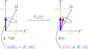
Figure 4: (color online). Schematic representation of the time evolution in the adiabatic frame, given by Eq. (13). The instantaneous eigenvector is represented by a thick blue arrow and the exact evolved state by a thick red arrow.

As depicted in Fig. 4, the evolved state in the original frame is given by

$$|{\psi(t)}\rangle=A(t)\,U_{\rm tr}(t)\,A^{-1}(0)\,|{\psi(0)}\rangle\,,$$ (13)

where the time evolution operator in the adiabatic frame is given by $U_{\rm tr}=e^{-iH_{\rm tr}t/\hbar}$. The fidelity at time $t=T$ can be obtained exactly:

$$F(T) =\frac{1}{4}\Bigl{[}\,\cos^{2}(\Omega T)(1+\cos^{2}\alpha)^{2}+4\sin^{2}(\Omega T)\cos^{2}\alpha$$

$$+2\cos(\Omega T)\sin^{2}\alpha(1+\cos^{2}\alpha)+\sin^{4}\alpha\,\Bigr{]}\,.$$ (14)

The results are indistinguishable from the numerical solution shown in Fig. 3(a). Perfect fidelity occurs at the resonance condition $\Omega T=2\pi n$, which is given by

$$JT/\hbar\pi=\sqrt{n^{2}-\frac{1}{16}}\approx n\,,\quad n\in\mathbb{N}\,.$$ (15)

We have now identified two paths to perfect teleportation. The first corresponds to the asymptotic (adiabatic) limit on the far right-hand side of Fig. 3. The second occurs at any one of the resonant conditions. It is interesting that resonances only occur in certain interpolation schemes. For example, the quadratic interpolation $f(s)=1-s^{2}$ and $g(s)=s(2-s)$ has resonances, while $f(s)=1-s^{2}$ and $g(s)=s^{2}$ does not.

Our results can be tested experimentally using current technology. Controllable three-qubit systems have been demonstrated in quantum dots Gaudreau12 and superconductors Martinis11 . Single-shot measurements and the preparation of singlet states are almost routine Buluta11 . AQT could therefore be implemented as follows. Qubit 1 is initially prepared in the “up” state, while qubits 2 and 3 are prepared in a singlet state. After switching $f$ and $g$ according to the AQT protocol, qubit 3 is measured. Repeating this experiment many times provides a fidelity estimate for AQT, over the evolution period $T$. The resonant peaks of the fidelity can be examined in the time domain by varying $T$. Since AQT corresponds to two parallel APs for the two spin components of a qubit, we could also explore interesting phenomena like coherent population trapping and electromagnetically induced transparency Scully , which have also been studied in the context of AP, for three-level atoms.

So far we have only explored AQT with three qubits, where qubits $2$ and $3$ are initially in a singlet state – the same initial state used for conventional quantum teleportation. An interesting next step would be to study AQT over longer distances. Our preliminary numerical studies suggest that AQT could be implemented in a more general spin chain geometry. We leave this for future work.

In conclusion, we have shown that adiabatic quantum teleportation consists of two adiabatic passages corresponding to the quantum information transfer of “up” and “down” components of a qubit. When this protocol is performed non-adiabatically, resonances occur in the fidelity, in analogy with magnetic spin resonance. The observation of resonances points toward a new paradigm for fast and robust adiabatic gates. Our results can be tested experimentally using superconducting or spin qubits, with currently available technologies.

- (1) P. W. Shor, Phys. Rev. A52, R2493 (1995).
- (2) J. Preskill, Proc. R. Soc. A 454, 385 (1998).
- (3) B. P. Lanyon, C. Hempel, D. Nigg, M. Müller, R. Gerritsma, F. Zähringer, P. Schindler, J. T. Barreiro, M. Rambach, G. Kirchmair, M. Hennrich, P. Zoller, R. Blatt, and C. F. Roos, Science 334, 57 (2011).
- (4) A. Messiah, Quantum Mechanics, (North-Holland Publishing Company, Amsterdam,1963).
- (5) W. D. Oliver, Y. Yu, J. C. Lee, K. K. Berggren, L. S. Levitov, and T. P. Orlando, Science 310, 1653 (2005).
- (6) L. Gaudreau, G. Granger, A. Kam, G. C. Aers, S. A. Studenikin, P. Zawadzki, M. Pioro-Ladrière, Z. R. Wasilewski, and A. S. Sachrajda, Nat. Phys. 8, 54 (2012).
- (7) J. Oreg, F. T. Hioe, and J. H. Eberly, Phys. Rev. A29 690 (1984).
- (8) K. Bergmann, H. Theuer, and B. W. Shore, Rev. Mod. Phys. 70, 1003 (1998).
- (9) P. Král, I. Thanopulos, and M. Shapiro, Rev. Mod. Phys. 79, 53 (2007).
- (10) B. W. Shore, Acta Physica Slovaca 58, 243 (2008).
- (11) Y.-x. Liu, J. Q. You, L. F. Wei, C. P. Sun, and F. Nori, Phys. Rev. Lett. 95, 087001 (2005); L.F. Wei, J. R. Johansson, L. X. Cen, S. Ashhab, and F. Nori, ibid. 100, 113601 (2008).
- (12) A. D. Greentree, J. H. Cole, A. R. Hamilton, and L. C. L. Hollenberg, Phys. Rev. B70, 235317 (2004).
- (13) E. Farhi, J. Goldstone, S. Gutmann, J. Lapan, A. Lundgren, and D. Preda, Science 292, 472 (2001).
- (14) D. Bacon and S. T. Flammia, Phys. Rev. Lett. 103, 120504 (2009).
- (15) M. Mariantoni, H. Wang, R. C. Bialczak, M. Lenander, E. Lucero, M. Neeley, A. D. O’Connell, D. Sank, M. Weides, J. Wenner, T. Yamamoto, Y. Yin, J. Zhao, J. M. Martinis, and A. N. Cleland, Nat. Phys. 7, 287 (2011).
- (16) The problem can also be solved using a SU(2) group method; see C. E. Carroll and F. T. Hioe, Phys. Rev. A42, 1522 (1990).
- (17) C. P. Slichter Principle of Magnetic Resonance, 3rd ed., (Springer-Verlag, NY, 1989).
- (18) C. Cohen-Tannoudji, B. Dui, and F. Laloë, Quantum Mechanics (John Wiley & Sons, NY, 1977).
- (19) I. Buluta, S. Ashhab, and F. Nori, Rep. Prog. Phys. 74, 104401 (2011).
- (20) M. O. Scully and M. S. Zubairy, Quantum Optics, (Cambridge Univ. Press, Cambridge, England, 1997).