New Measurements of Upsilon Spin Alignment at the Tevatron

Abstract

We describe a new analysis of $\Upsilon(nS)\rightarrow\mu^{+}\mu^{-}$ decays collected in $p\overline{p}$ collisions with the CDF II detector at the Fermilab Tevatron. This analysis measures the angular distributions of the final state muons in the $\Upsilon$ rest frame, providing new information about $\Upsilon$ production polarization. We find the angular distributions to be nearly isotropic up to $\Upsilon$ $p_{T}$ of $40\;{\rm GeV}/c$, consistent with previous measurements by CDF, but inconsistent with results obtained by the D0 experiment. The results are compared with recent NLO calculations based on color-singlet matrix elements and non-relativistic QCD with color-octet matrix elements.

1 Introduction

A recent analysis bib-arxiv of $\Upsilon\rightarrow\mu^{+}\mu^{-}$ decays collected with the CDF II detector provides new measurements of the distributions of decay angles, which depend on the polarization of $\Upsilon$ states produced in $p\overline{p}$ collisions. Previous measurements bib-cdf ; bib-d0 carried out by the CDF and D0 experiments provided useful, but incomplete information about these angular distributions and did not strongly favor the predictions of any of the models bib-kt ; bib-co used to calculate the production cross sections. Furthermore, the fact that these previous measurements are in apparent disagreement has led to the speculation that significant acceptance biases could have been overlooked, motivating the need to perform additional tests of internal consistency in future measurements bib-faccioli .

The analysis described here measures the full angular distributions of the final state muons from $\Upsilon(1S)$, $\Upsilon(2S)$, and $\Upsilon(3S)$ decays as functions of the $\Upsilon$ transverse momentum up to $40\;{\rm GeV}/c$. This is the first analysis to report measurements of the $\Upsilon(3S)$ spin alignment. It is also the first analysis to measure spin alignment in two different coordinate frames and to compare rotationally invariant quantities in these frames to demonstrate internal consistency.

2 Analysis Overview

In the rest frame of the $\Upsilon$ decay, the direction of the positive muon is described using polar angles $(\theta,\varphi)$ measured with respect to a given set of coordinate axes. The $s$–channel helicity frame, used in earlier analyses, defined the $z$-axis along the $\Upsilon$ momentum vector, with the $x$-axis in the production plane and the $y$-axis perpendicular to both $x$- and $z$-axes. Alternatively, the Collins–Soper frame bib-cs can be used for which the $z$-axis approximates, on average, the direction of the velocity of the colliding partons. The form of the angular distribution is constrained by angular momentum conservation; for a vector meson decaying to two fermions it can be written

$$\frac{dN}{d\Omega} \sim 1+\lambda_{\theta}\cos^{2}\theta+\lambda_{\varphi}\sin^{2}\theta\cos 2\varphi+\lambda_{\theta\varphi}\sin 2\theta\cos\varphi+$$ (1)

$$\lambda_{\varphi}^{\perp}\sin^{2}\theta\sin 2\varphi+\lambda_{\theta\varphi}^{\perp}\sin 2\theta\sin\varphi.$$

A four-fold symmetry in the acceptance may be exploited to increase statistics in small bins of solid angle by combining $(\theta,\varphi)$ with $(\theta,-\varphi)$ and $(\theta,\varphi)$ with $(\pi-\theta,\pi-\varphi)$, although this leads to a cancellation of the terms with $\lambda^{\perp}_{\varphi}$ and $\lambda^{\perp}_{\theta\varphi}$ as coefficients. The coefficients quantify the shape of the angular distribution and provide direct information about the polarization of the ensemble of $\Upsilon$ states since they are related to the elements of the spin density matrix elements $\rho_{ij}$ bib-noman by the expressions $\lambda_{\theta}=(\rho_{11}-\rho_{00})/(\rho_{11}+\rho_{00})$, $\lambda_{\varphi}=\rho_{10}/(\rho_{11}+\rho_{00})$, and $\lambda_{\theta\varphi}=\rho_{1,-1}/(\rho_{11}+\rho_{00})$.

When a sample of $\Upsilon$ decays is selected using a dimuon trigger, the observed angular distribution will differ from the form in Eq. (1) because of the limited acceptance imposed by the muon $p_{T}$ thresholds in the trigger and the geometric coverage of the detector systems. The acceptance can change rapidly with both the transverse momentum and mass of the dimuon system but can be calculated accurately using a combination of Monte Carlo simulations, which model the detector geometry, and trigger efficiencies measured using independent data samples. The angular distributions of dimuons with mass that include one of the $\Upsilon(nS)$ resonances will depend strongly on angular distributions present in non-resonant backgrounds, which can be highly non-isotropic. These may have angular distributions that can be parameterized using Eq. (1), but they could be more complex since they do not necessarily arise from the decay of a single vector state.

2.1 Previous Analyses

Previous $\Upsilon$ spin alignment analyses bib-cdf ; bib-d0 were performed using only the $s$–channel helicity frame and integrated angular distributions over $\varphi$, retaining only sensitivity to the coefficient $\lambda_{\theta}$ which is frequently denoted $\alpha$ in the literature. This was carried out in several ranges of $p_{T}(\Upsilon)$ by fitting the dimuon mass distribution in discrete ranges of $\cos\theta$ to determine the $\Upsilon$ yields, correcting for detector acceptance, and fitting the resulting distributions to a function of the form $1+\alpha\cos^{2}\theta$. In practice, this is not a trivial procedure because both the $\Upsilon$ acceptance and the shape of the background mass distribution change significantly with both $p_{T}$ and $\cos\theta$.

The limitations of these analyses have been pointed out for several years now bib-faccioli . The measurement of only one of the three coefficients in Eq. (1) does not allow the calculation of rotationally invariant quantities or the transformation $\lambda_{\theta}$ from the $s$–channel helicity frame to different coordinate systems. This procedure also does not generalize well to the analysis in many small bins of $\cos\theta$ and $\varphi$ because the large number of fits to invariant mass distributions with poorly constrained background shapes may suffer from large statistical fluctuations or systematic biases.

2.2 A New Approach

The analysis procedure described here divides $(\cos\theta,\varphi)$ into $20\times 36$ bins, but it avoids the need to measure $\Upsilon$ yields in each bin separately. Instead, all dimuon events with invariant mass near each of the $\Upsilon$ signals are selected and the observed numbers of events in each bin are modeled using separate angular distributions of the form in Eq. (1) for signal and background, multiplied by the detector acceptance which is calculated in each individual bin. The parameters $\lambda_{\theta}$, $\lambda_{\varphi}$, $\lambda_{\theta\varphi}$ corresponding to the angular distribution of the $\Upsilon$ signal can then be measured provided the amount of background and its angular distribution are known.

Within a given range of dimuon $p_{T}$, the amount of background under the $\Upsilon(nS)$ signals is determined from a fit to their invariant mass distribution but an independent sample is needed to constrain the shape of the angular distribution from background sources. Such a sample is obtained by demanding that the extrapolated trajectory of at least one of the muons misses the average beam axis by a distance $|d_{0}|>150\;{\rm\mu m}$. Although this “displaced” muon sample contains a few percent of the $\Upsilon$ signal due to the $d_{0}$ measurement resolution, it mostly selects muons produced in semileptonic decays of heavy quarks, which forms the dominant source of background. Since the impact parameter requirement does not bias the muon decay angle, the angular distribution of muons from background sources is expected to be the same in the complementary “prompt” muon sample.

A simultaneous fit is then performed to the angular distributions of dimuon events in prompt and displaced samples selected from ranges of invariant mass around each of the $\Upsilon$ signals. In each bin of $p_{T}(\Upsilon)$, the fit is performed by maximizing the likelihood function constructed from the probabilities of obtaining the observed numbers of events in bins of $(\cos\theta,\varphi)$ given expected yields calculated using

$$\frac{dN_{p}}{d\Omega_{ij}} \sim N_{\Upsilon}f_{p}{\cal A}_{\Upsilon}(\cos\theta_{i},\varphi_{j})\cdot w_{\Upsilon}(\cos\theta_{i},\varphi_{j};\bar{\lambda}_{\Upsilon})+$$ (2)

$$N_{d}s_{p}{\cal A}_{b}(\cos\theta_{i},\varphi_{j})\cdot w_{b}(\cos\theta_{i},\varphi_{j};\bar{\lambda}_{b}),$$

$$\frac{dN_{d}}{d\Omega_{ij}} \sim N_{\Upsilon}(1-f_{p}){\cal A}_{\Upsilon}(\cos\theta_{i},\varphi_{j})\cdot w_{\Upsilon}(\cos\theta_{i},\varphi_{j};\bar{\lambda}_{\Upsilon})+$$ (3)

$$N_{d}{\cal A}_{b}(\cos\theta_{i},\varphi_{j})\cdot w_{b}(\cos\theta_{i},\varphi_{j};\bar{\lambda}_{b}).$$

In these expressions, $N_{\Upsilon}$ and $N_{d}$ are the numbers of $\Upsilon$ and displaced background events, $f_{p}$ is the fraction of the $\Upsilon$ signal retained in the prompt sample, and $s_{p}$ is the ratio of the background yields in prompt and displaced samples. The parameters $f_{p}$ and $s_{p}$ are constrained using fits to the prompt and displaced mass distributions. The acceptance ${\cal A}_{\Upsilon}$ for $\Upsilon$ signal and ${\cal A}_{b}$ for dimuon background events are calculated using Monte Carlo simulations and the measured trigger and muon selection efficiencies. The underlying angular distribution of muons from $\Upsilon$ decays, $w_{\Upsilon}$, is calculated using Eq. (1) with coefficients denoted collectively as $\bar{\lambda}_{\Upsilon}$. The angular distribution of muons in the background component, $w_{b}$, is similar, but has an additional term, described below, that allows a better description of the data.

3 Analysis of CDF Data

3.1 Upsilon Trigger

The analysis of $\Upsilon\rightarrow\mu^{+}\mu^{-}$ decays is performed at CDF using a sample of events collected with a 3-level dimuon trigger. This trigger required the presence of two oppositely charged tracks at level 1 with $p_{T}>1.5\;{\rm GeV}/c$ that extrapolate to hits in one of the CDF muon detector systems bib-xft . At least one of the muons had to be in the central region and the level 2 trigger required that it was also detected in a second muon detector system located behind additional steel absorber. After full event reconstruction, the level 3 trigger required that this muon had $p_{T}>4\;{\rm GeV}/c$, the other muon had $p_{T}>3\;{\rm GeV}/c$ and that the invariant mass of the pair was between $8$ and $12\;{\rm GeV}/c^{2}$. The geometric acceptance of these triggers restricts the rapidity of the $\Upsilon$ sample to the central region, $|y(\Upsilon)|<0.6$.

For most of Run II, the level 2 trigger was prescaled dynamically to maintain an approximately constant accept rate and dead time, but more recently, the level 1 trigger was disabled when instantaneous luminosities were greater than $280\times 10^{30}\;{\rm cm}^{-2}{\rm s}^{-1}$. The prescaled triggers integrated approximately 70% of the delivered luminosity, averaged over the first $6.7\;{\rm fb}^{-1}$ of data collected in Run II. Figure 1 shows the mass distribution of dimuons collected using these triggers that are used in the angular analysis.

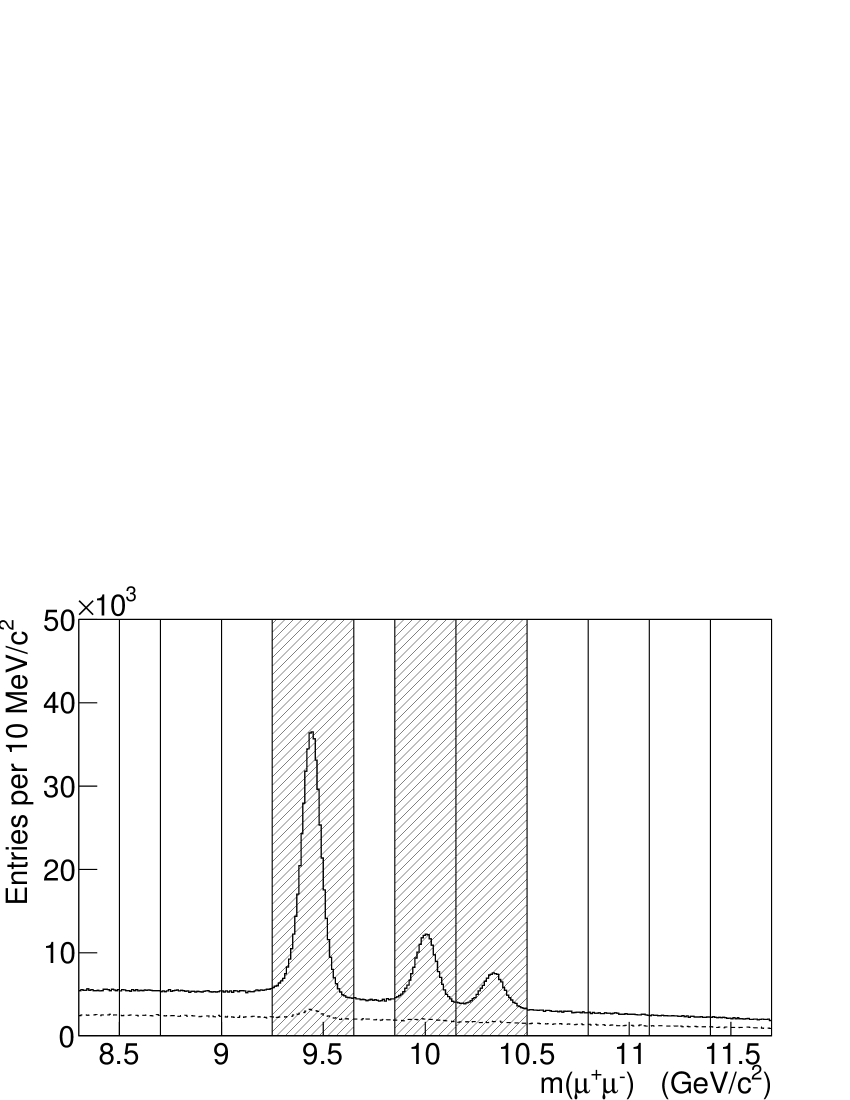
Figure 1: Distribution of $\mu^{+}\mu^{-}$ invariant mass. Pairs where both originate from close to the beam axis are indicated by the solid histogram, while those for which at least one misses the beamline by more than $150\;{\rm\mu m}$ are shown in the dashed histogram. The shaded regions indicate the range of masses used to select the $\Upsilon(1S)$, $\Upsilon(2S)$ and $\Upsilon(3S)$ states, while the other regions are used to study background properties.

3.2 Angular Distributions in Background Events

The analysis of the angular distributions of muons from $\Upsilon$ decays relies on accurately subtracting the angular distributions that are present in the background which are estimated using the displaced track sample. The validity of this procedure is checked by comparing the observed distribution of decay angles in the high and low mass sideband regions. The example shown in Fig. 2 demonstrates that this is the case, with consistency between the two samples tested by computing the Kolmogorov–Smirnov statistic.

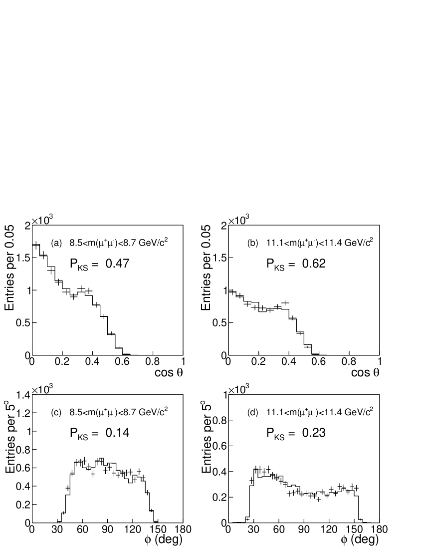
Figure 2: Comparisons of $\cos\theta$ (a,b) and $\varphi$ (c,d) distributions, measured in the Collins–Soper frame, for prompt and displaced samples (histograms and error bars, respectively). Reasonable agreement, quantified by computing the Kolmogorov–Smirnov statistic, is observed in mass regions both below (a,c) the $\Upsilon(1S)$ and above (b,d) the $\Upsilon(3S)$ resonances.

3.3 Simultaneous Fit in Signal Regions

The similarities observed in the angular distributions of prompt and displaced muon samples at masses both above and below the $\Upsilon(nS)$ resonances support the use of the displaced muon sample to model the background properties under the $\Upsilon$ signals. Thus, we apply the simultaneous fit to prompt and displaced muon samples with mass selected from each of the three regions containing the $\Upsilon$ signals indicated in Fig. (1). To accommodate the description of the angular distribution of the background, which is observed to be very non-isotropic, an additional term proportional to $\cos^{4}\theta$ is added to Eq. (1) to obtain the functiona used for $w_{b}$. In addition, a component of the sample that is strongly peaked at large values of $\cos\theta$ in the $s$–channel helicity frame is removed by requiring that $|p_{T}(\mu^{+})-p_{T}(\mu^{-})|<(p_{T}(\mu^{+}\mu^{-})-0.5\;{\rm GeV}/c)$. This restriction is included in the calculation of the $\Upsilon$ acceptance but has a negligible effect for $p_{T}(\Upsilon)>6\;{\rm GeV}/c$.

The quality of the resulting fit is assessed by comparing projections of the angular distributions observed in the data with the corresponding projections of the fit. Fig. 3 shows an example of projections for muon pairs selected from the mass range containing the $\Upsilon(1S)$ signal.

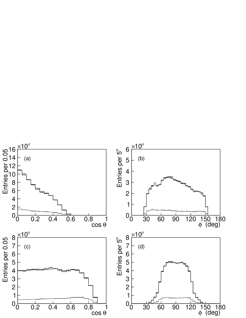
Figure 3: Projections of angular distributions measured in the Collins–Soper frame (a,b) and the $s$–channel helicity frame (c,d) for muon pairs with $4<p_{T}<6\;{\rm GeV}/c$ and mass in the vicinity of the $\Upsilon(1S)$ signal. The projected distributions in the data are indicated with error bars for the prompt (black) and displaced (gray) samples. Solid histograms show the projections of the fits.

The quality of fits applied to the other kinematic regions is similar and shows no systematic trends that depend on either $p_{T}(\mu^{+}\mu^{-})$ or their invariant mass.

3.4 Results

The new measurements of $\lambda_{\theta}$ for the $\Upsilon(1S)$ state can be compared with previous results from the CDF and D0 experiments and with recent NLO predictions bib-qwg ; bib-nrqcd ; bib-csm . These are shown in Fig. 4 from which it is apparent that although the new results are consistent with the Run I CDF measurement, they are inconsistent with D0 analysis, with the significance estimated to be approximately $4.5\sigma$.

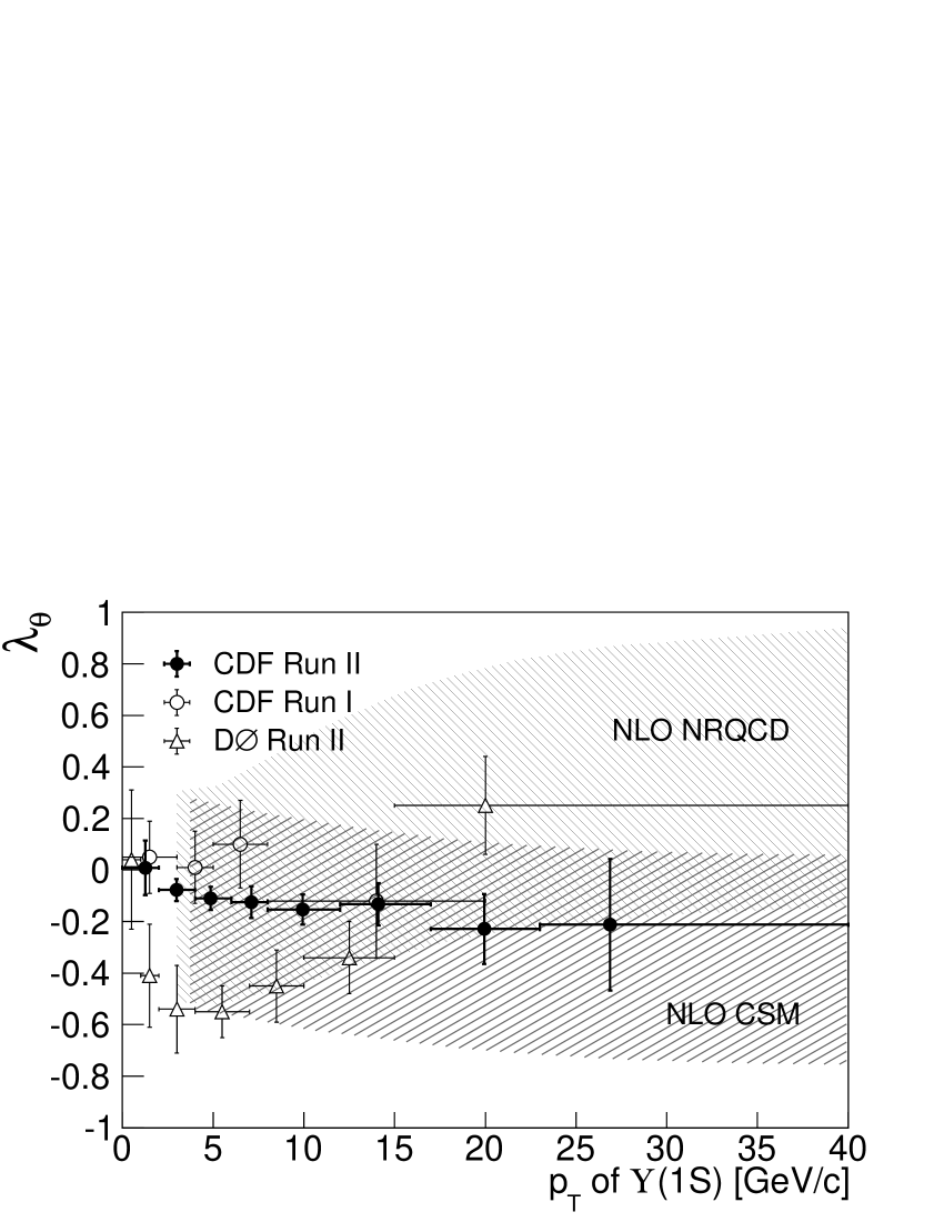
Figure 4: Measurements of $\lambda_{\theta}$ in the $s$–channel helicity frame for the $\Upsilon(1S)$ state compared with previous results from CDF (with $|y(\Upsilon)|<0.4$) and D0 (with $|y|<1.8$) and with next-to-leading order calculations based on NRQCD with color-octet matrix elements, and a next-to-leading order color-singlet model.

The theoretical predictions are currently somewhat imprecise due to the poorly measured production cross sections for $\chi_{bJ}(nP)$ states that decay into $\Upsilon(1S)$ bib-cdfchib , but recent results from the ATLAS experimentbib-atlas may improve on this situation.

4 Rotational Invariants

We also demonstrate the internal consistency of the results by calculating the rotational invariant $\tilde{\lambda}=(\lambda_{\theta}+3\lambda_{\varphi})/(1-\lambda_{\varphi})$ using the values of $\lambda_{\theta}$ and $\lambda_{\varphi}$ measured in the $s$–channel helicity frame and the Collins–Soper frames. Agreement between the values calculated in each coordinate frame is an important consistency test because poor determination of the experimental acceptance or inaccuracies in the subtraction of the highly non-isotropic backgrounds would be expected to introduce coordinate frame dependent biases in the measured angular distributions.

The value of $\tilde{\lambda}$ quantifies the shape of the angular distribution independent of its orientation with respect to a coordinate frame. Decays of $\Upsilon$ states with pure transverse polarization yield angular distributions with $\tilde{\lambda}=+1$ while a purely longitudinal polarization gives $\tilde{\lambda}=-1$. A value of $\tilde{\lambda}=0$ correspond to an isotropic angular distribution, which cannot result from the decay of a pure spin-1 state but instead would indicate that multiple production mechanisms are present leading to an effectively unpolarized ensemble of decays.

Figure 5 shows the values of $\tilde{\lambda}$ measured for the $\Upsilon(1S)$, $\Upsilon(2S)$ and $\Upsilon(3S)$ states as functions of $p_{T}(\Upsilon)$ in both the Collins–Soper and the $s$–channel helicity frames.

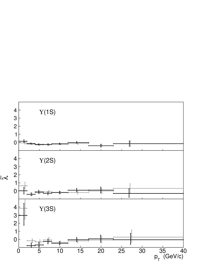
Figure 5: Rotational invariant $\tilde{\lambda}$, measured in the Collins–Soper frame (dark lines) and $s$–channel helicity frame (gray lines) as functions of $p_{T}(\Upsilon)$.

Since $\tilde{\lambda}$ is measured in each coordinate frame using the same data samples, the statistical uncertainty of each measurement is highly correlated. The sizes of variations in values of $\tilde{\lambda}$ measured in the two frames that would be expected from purely statistical fluctuations were estimated using Monte Carlo simulations and found to be generally consistent with the observed differences. This is the first analysis to perform such a test and based on these findings, there appears to be no evidence for significant biases in the calculated acceptance.

The values $\tilde{\lambda}\approx 0$ reached at large $p_{T}$ suggest that all three of the $\Upsilon(nS)$ states are produced in an unpolarized mixture. This is the first measurement of angular distributions in $\Upsilon(3S)$ decays and is significant because it had been thought that a greater fraction of $3S$ states should be produced directly, rather than via feed-down from $\chi_{b}$ states, in which case the calculated spin alignment predictions should be more precise.

5 Conclusions

The measurements described here provide the most detailed characterization of the angular distributions of $\Upsilon\rightarrow\mu^{+}\mu^{-}$ decays produced at a hadron collider to date. We find little evidence for strong polarization of any of the three $\Upsilon(nS)$ states in the central region of rapidity $|y|<0.6$ and with $p_{T}$ up to $40\;{\rm GeV}/c$. This is consistent with the results previously obtained in Run I by CDF and inconsistent with measurements carried out by D0 in Run II. Although the D0 measurements were carried out over the wider range of rapidity $|y(\Upsilon)|<1.8$, we find no evidence that the angular distributions change rapidly in the central region of rapidity accessible to the CDF detector. We look forward to the possibility of refined predictions from theory and new results from the LHC experiments which may be able to further clarify the experimental situation.

References

- (1) T. Aaltonen et al. (the CDF Collaboration), arXiv:1112.1591 [hep-ex] (submitted to Phys. Rev. Lett.)
- (2) D. Acosta et al. (CDF Collaboration), Phys. Rev. Lett. 88, 161802 (2002).
- (3) V.M. Abazov et al. (D0 Collaboration), Phys. Rev. Lett. 101, 182004 (2008).
- (4) P. Cho and A.K. Leibovich, Phys. Rev. D 53, 150 (1996); 53, 6203 (1996).
- (5) S.P. Baranov and N.P. Zotov, JETP Lett. 86, 435 (2007).
- (6) P. Faccioli, C. Lourenço, J. Seixas, and H. K. Wohri, Phys. Rev. Lett. 102, 151802 (2009); Eur. Phys. J. C 69, 657 (2010); P. Faccioli, C. Lourenço, and J. Seixas, Phys. Rev. Lett. 105, 061601 (2010); Phys. Rev. D 81, 111502(R) (2010).
- (7) J.C. Collins and D.E. Soper, Phys. Rev. D 16, 2219 (1977).
- (8) M. Noman and S. D. Rindani, Phys. Rev. D 19, 207 (1979).
- (9) E. J. Thomson et al., IEEE Trans. Nucl. Sci. 49, 1063 (2002).
- (10) Z. Conessa del Valle et al., Nucl. Phys. B (proc. Suppl.) 214, 3 (2011).
- (11) B. Gong, J.-X. Wang and H.-F. Zhang, Phys. Rev. D 83, 114021 (2011).
- (12) P. Artoisenet et al., Phys. Rev. Lett. 101, 152001 (2008).
- (13) T. Affolder et al. (the CDF Collaboration), Phys. Rev. Lett. 84, 2094 (2000).
- (14) G. Aad et al. (the ATLAS Collaboration), arXiv:1112.5154 [hep-ex] (submitted to Phys. Rev. Lett.)