Space Shift Keying (SSK–) MIMO with Practical Channel Estimates

Abstract

In this paper, we study the performance of space modulation for Multiple–Input–Multiple–Output (MIMO) wireless systems with imperfect channel knowledge at the receiver. We focus our attention on two transmission technologies, which are the building blocks of space modulation: i) Space Shift Keying (SSK) modulation; and ii) Time–Orthogonal–Signal–Design (TOSD–) SSK modulation, which is an improved version of SSK modulation providing transmit–diversity. We develop a single–integral closed–form analytical framework to compute the Average Bit Error Probability (ABEP) of a mismatched detector for both SSK and TOSD–SSK modulations. The framework exploits the theory of quadratic–forms in conditional complex Gaussian Random Variables (RVs) along with the Gil–Pelaez inversion theorem. The analytical model is very general and can be used for arbitrary transmit– and receive–antennas, fading distributions, fading spatial correlations, and training pilots. The analytical derivation is substantiated through Monte Carlo simulations, and it is shown, over independent and identically distributed (i.i.d.) Rayleigh fading channels, that SSK modulation is as robust as single–antenna systems to imperfect channel knowledge, and that TOSD–SSK modulation is more robust to channel estimation errors than the Alamouti scheme. Furthermore, it is pointed out that only few training pilots are needed to get reliable enough channel estimates for data detection, and that transmit– and receive–diversity of SSK and TOSD–SSK modulations are preserved even with imperfect channel knowledge.

I Introduction

Space modulation [1] is a novel digital modulation concept for Multiple–Input–Multiple–Output (MIMO) wireless systems, which is receiving a growing attention due to the possibility of realizing low–complexity and spectrally–efficient MIMO implementations [2]–[7]. The space modulation principle is known in the literature in various forms, such as Information–Guided Channel Hopping (IGCH) [2], Spatial Modulation (SM) [3], and Space Shift Keying (SSK) modulation [4]. Although different from one another, all these transmission technologies share the same fundamental working principle, which makes them unique with respect to conventional modulation schemes: they encode part of the information bits into the spatial positions of the transmit–antennas in the antenna–array, which plays the role of a constellation diagram (the so–called “spatial–constellation diagram”) for data modulation [1], [7]. In particular, SSK modulation exploits only the spatial–constellation diagram for data modulation, which results in a very low–complexity modulation concept for MIMO systems [4]. Recently, improved space modulation schemes that can achieve a transmit–diversity gain have been proposed in [8]–[11]. Furthermore, a unified MIMO architecture based on the SSK modulation principle has been introduced in [12].

In SSK modulation, blocks of information bits are mapped into the index of a single transmit–antenna, which is switched on for data transmission while all the other antennas radiate no power [4]. SSK modulation exploits the location–specific property of the wireless channel for data modulation [7]: the messages sent by the transmitter can be decoded at the destination since the receiver sees a different Channel Impulse Response (CIR) on any transmit–to–receive wireless link. In [4] and [7], it has been shown that the CIRs are the points of the spatial–constellation diagram, and that the Bit Error Probability (BEP) depends on the distance among these points. Recent results have shown that, if the receiver has Perfect Channel State Information (P–CSI), space modulation can provide better performance than conventional modulation schemes with similar complexity [2]–[4], [9], [10], and [13]–[17]. However, due to its inherent working principle, the major criticism about the adoption of SSK modulation in realistic propagation environments is its robustness to the imperfect knowledge of the wireless channel at the receiver. In particular, it is often argued that space modulation is more sensitive to channel estimation errors than conventional systems. The main contribution of this paper is to shed light on this matter.

Some research works on the performance of space modulation with imperfect channel knowledge are available in the literature. However, they are insufficient and only based on numerical simulations. In [4], the authors have studied the ABEP of SSK modulation with non–ideal channel knowledge. However, there are four limitations in this paper: i) the ABEP is obtained only through Monte Carlo simulations, which is not very much insightful; ii) the arguments in [4] are applicable only to Gaussian fading channels and do not take into account the cross–product between channel estimation error and Additive White Gaussian Noise (AWGN) at the receiver; iii) it is unclear from [4] how the ABEP changes with the pilot symbols used by the channel estimator; and iv) the robustness/weakness of SSK modulation with respect to conventional modulation schemes is not analyzed. In [18], we have studied the performance of SSK modulation when the receiver does not exploit for data detection the knowledge of the phase of the channel gains (semi–blind receiver). It is shown that semi–blind receivers are much worse than coherent detection schemes, and, thus, that the assessment of the performance of coherent detection with imperfect channel knowledge is a crucial aspect for SSK modulation. A very interesting study has been recently conducted in [19], where the authors have compared the performance of SM and V–BLAST (Vertical Bell Laboratories Layered Space–Time) [20] schemes with practical channel estimates. It is shown that the claimed sensitivity of space modulation to channel estimation errors is simply a misconception and that, on the contrary, SM is more robust than V–BLAST to imperfections on the channel estimates, and that less training is, in general, needed. However, the study in [19] is conducted only through Monte Carlo simulations, which do not give too much insights for performance analysis and system optimization. Finally, in [10] the authors have proposed a Differential Space–Time Shift Keying (DSTSK) scheme, which is based on the Cayley unitary transform theory. The DSTSK scheme requires no channel estimation at the receiver, but incurs in a 3dB performance loss with respect to coherent detection. Furthermore, it can be applied to only real–valued signal constellations. Unlike [10], which avoids channel estimation, we are interested in studying the training overhead that is needed for channel estimation and to achieve close–to–optimal performance with coherent detection.

Motivated by these considerations, this paper is aimed at developing a very general analytical framework to assess the performance of space modulation with coherent detection and practical channel estimates. In particular, we focus our attention on two transmission technologies, which are the building blocks of space modulation: i) Space Shift Keying (SSK) modulation [4]; and ii) Time–Orthogonal–Signal–Design (TOSD–) SSK modulation, which is an improved version of SSK modulation providing transmit–diversity [8], [11]. Our theoretical and numerical results corroborate the findings in [19], and highlight three important outcomes: i) SSK modulation is as robust as single–antenna systems to imperfect channel knowledge; ii) TOSD–SSK modulation is more robust to channel estimation errors than the Alamouti scheme [21]; and iii) only few training pilots are needed to get reliable enough channel estimates for data detection. More precisely, we provide the following contributions: i) we develop a single–integral closed–form analytical framework to compute the Average BEP (ABEP) of a mismatched detector [22] for SSK and TOSD–SSK modulations, which can be used for arbitrary transmit– and receive–antennas, fading distributions, fading spatial correlations, and training pilots for channel estimation. It is shown that the mismatched detector of SSK and TOSD–SSK modulations can be cast in terms of a quadratic–form in complex Gaussian Random Variables (RVs) when conditioning upon fading channel statistics, and that the ABEP can be computed by exploiting the Gil–Pelaez inversion theorem [23]; ii) over independent and identically distributed (i.i.d.) Rayleigh fading channels, we show that SSK modulation is superior to Quadrature Amplitude Modulation (QAM), regardless of the number of training pulses, if the spectral efficiency is greater than 2 bpcu (bits per channel use) and the receiver has at least two antennas; iii) in the same fading channel, we show that TOSD–SSK modulation is superior, regardless of the number of antennas at the receiver and training pulses, to the Alamouti scheme with QAM if the spectral efficiency is greater than 2 bpcu. Also, unlike the P–CSI setup, TOSD–SSK modulation can outperform the Alamouti scheme if the spectral efficiency is 2 bpcu, just one pilot pulse for channel estimation is used, and the detector is equipped with at least two antennas; iv) still over i.i.d. Rayleigh fading, we show that, compared to the P–CSI scenario, SSK and TOSD–SSK modulations have a Signal–to–Noise–Ratio (SNR) penalty of approximately 3dB and 2dB when only one pilot pulse can be used for channel estimation, respectively. Also, single–antenna and Alamouti schemes have a SNR penalty of approximately 3dB for QAM; and v) we verify that transmit– and receive–diversity of SSK and TOSD–SSK modulations are preserved even for a mismatched detector.

The remainder of this paper is organized as follows. In Section II, the system model is introduced. In Section III and Section IV, SSK and TOSD–SSK modulations are described and the analytical frameworks to compute the ABEP with imperfect channel knowledge are developed, respectively. In Section V, the spectral efficiency of TOSD–SSK modulation with time–orthogonal shaping filters is studied. In Section VI, numerical results are shown to substantiate the analytical derivation, and to compare SSK and TOSD–SSK modulations with state–of–the–art single–antenna and Alamouti schemes. Finally, Section VII concludes this paper.

II System Model

We consider a generic $N_{t}\times N_{r}$ MIMO system, with $N_{t}$ and $N_{r}$ being the number of antennas at the transmitter and at the receiver, respectively. SSK and TOSD–SSK modulations work as follows [4], [8], [11]: i) the transmitter encodes blocks of $\log_{2}\left(N_{t}\right)$ data bits into the index of a single transmit–antenna, which is switched on for data transmission while all the other antennas are kept silent; and ii) the receiver solves an $N_{t}$–hypothesis detection problem to estimate the transmit–antenna that is not idle, which results in the estimation of the unique sequence of bits emitted by the encoder. With respect to SSK modulation [4], in TOSD–SSK modulation [11] the $t$–th transmit–antenna, when active, radiates a distinct pulse waveform ${w_{t}\left(\cdot\right)}$ for $t=1,2,\ldots,N_{t}$, and the waveforms across the antennas are time–orthogonal, i.e., $\int\nolimits_{-\infty}^{+\infty}{w_{t_{1}}\left(\xi\right)w_{t_{2}}^{*}\left(\xi\right)d\xi}=0$ if $t_{1}\neq t_{2}$ and $\int\nolimits_{-\infty}^{+\infty}{w_{t_{1}}\left(\xi\right)w_{t_{2}}^{*}\left(\xi\right)d\xi}=1$ if $t_{1}=t_{2}$. In other words, SSK modulation is a special case of TOSD–SSK modulation with $w_{t}\left(\xi\right)=w_{0}\left(\xi\right)$ for $t=1,2,\ldots,N_{t}$.

In [11], we have analytically proved that the diversity order of SSK modulation is $N_{r}$, while the diversity order of TOSD–SSK modulation is $2N_{r}$, which results in a transmit–diversity equal to 2 and a receive–diversity equal to $N_{r}$. Thus, TOSD–SSK modulation provides a full–diversity–achieving (i.e., the diversity gain is $N_{t}N_{r}$) system if $N_{t}=2$. This scheme has been recently generalized in [24] to achieve arbitrary transmit–diversity. It is worth emphasizing that in TOSD–SSK modulation a single–antenna is active for data transmission and that the information bits are still encoded into the index of the transmit–antenna, and are not encoded into the impulse (time) response, ${w_{t}\left(\cdot\right)}$, of the shaping filter. In other words, TOSD–SSK modulation is different from conventional Single–Input–Single–Output (SISO) schemes with Orthogonal Pulse Shape Modulation (O–PSM) [25], which are unable to achieve transmit–diversity as only a single wireless link is exploited for communication [11]. Also, TOSD–SSK modulation is different from conventional transmit–diversity schemes [26], and requires no extra time–slots for transmit–diversity. Further details are available in [11] and are here omitted to avoid repetitions.

Throughout this paper, the block of information bits encoded into the index of the $t$–th transmit–antenna is called “message”, and it is denoted by $m_{t}$ for $t=1,2,\ldots,N_{t}$. The $N_{t}$ messages are assumed to be equiprobable. Moreover, the related transmitted signal is denoted by $s_{t}\left(\cdot\right)$. It is implicitly assumed with this notation that, if $m_{t}$ is transmitted, the analog signal $s_{t}\left(\cdot\right)$ is emitted by the $t$–th transmit–antenna while the other antennas radiate no power.

II-A Notation

Main notation is as follows. i) We adopt a complex–envelope signal representation. ii) $j=\sqrt{-1}$ is the imaginary unit. iii) $\left({x\otimes y}\right)\left(u\right)=\int_{-\infty}^{+\infty}{x\left(\xi\right)y\left({u-\xi}\right)d\xi}$ is the convolution of signals $x\left(\cdot\right)$ and $y\left(\cdot\right)$. iv) $\left|{\cdot}\right|^{2}$ is the square absolute value. v) $\textrm{E}\left\{\cdot\right\}$ is the expectation operator computed over channel fading statistics. vi) ${\mathop{\rm Re}\nolimits}\left\{\cdot\right\}$ and ${\mathop{\rm Im}\nolimits}\left\{\cdot\right\}$ are real and imaginary part operators, respectively. vii) $\Pr\left\{\cdot\right\}$ denotes probability. viii) $Q\left(u\right)=\left({{1\mathord{\left/{\vphantom{1{\sqrt{2\pi}}}}\right.\kern-1.2pt}{\sqrt{2\pi}}}}\right)\int_{u}^{+\infty}{\exp\left({-{{\xi^{2}}\mathord{\left/{\vphantom{{\xi^{2}}2}}\right.\kern-1.2pt}2}}\right)d\xi}$ is the Q–function. ix) $\delta\left(\cdot\right)$ and $\delta_{\cdot,\cdot}$ are Dirac and Kronecker delta functions, respectively. x) $M_{X}\left(s\right)=\textrm{E}\left\{{\exp\left({sX}\right)}\right\}$ and $\Psi_{X}\left(\nu\right)=\textrm{E}\left\{{\exp\left({j\nu X}\right)}\right\}$ are Moment Generating Function (MGF) and Characteristic Function (CF) of RV $X$, respectively. xi) $\propto$ denotes “is proportional to”.

II-B Channel Model

We consider a general frequency–flat slowly–varying channel model with generically correlated and non–identically distributed fading gains. In particular ($t=1,2,\ldots,N_{t}$, $r=1,2,\ldots,N_{r}$):

• $h_{t,r}\left(\xi\right)=\alpha_{t,r}\delta\left({\xi-\tau_{t,r}}\right)$ is the channel impulse response of the transmit–to–receive wireless link from the $t$–th transmit–antenna to the $r$–th receive–antenna. $\alpha_{t,r}=\beta_{t,r}\exp\left({j\varphi_{t,r}}\right)$ is the complex channel gain with $\beta_{t,r}$ and $\varphi_{t,r}$ denoting the channel envelope and phase, respectively, and $\tau_{t,r}$ is the propagation time–delay.

• The time–delays $\tau_{t,r}$ are assumed to be known at the receiver, i.e., perfect time–synchronization is considered. Furthermore, we consider $\tau_{1,1}\cong\tau_{1,2}\cong\ldots\cong\tau_{N_{t},N_{r}}$, which is a realistic assumption when the distance between the transmitter and the receiver is much larger than the spacing between the transmit– and receive–antennas [7]. Due to the these assumptions, the propagation delays can be neglected in the remainder of this paper.

II-C Channel Estimation

Let $E_{p}$ and $N_{p}$ be the energy transmitted for each pilot pulse and the number of pilot pulses used for channel estimation, respectively. Similar to [27] and [28], we assume that channel estimation is performed by using a Maximum–Likelihood (ML) detector, and by observing $N_{p}$ pilot pulses that are transmitted before the modulated data. During the transmission of one block of pilot–plus–data symbols, the wireless channel is assumed to be constant, i.e. a quasi–static channel model is considered. With these assumptions, the estimates of channel gains $\alpha_{t,r}$ ($t=1,2,\ldots,N_{t}$, $r=1,2,\ldots,N_{r}$) can be written as follows:

$$\hat{\alpha}_{t,r}=\hat{\beta}_{t,r}\exp\left({j\hat{\varphi}_{t,r}}\right)=\alpha_{t,r}+\varepsilon_{t,r}$$ (1)

where $\hat{\alpha}_{t,r}$, $\hat{\beta}_{t,r}$, and ${\hat{\varphi}_{t,r}}$ are the estimates of $\alpha_{t,r}$, $\beta_{t,r}$, and ${\varphi_{t,r}}$, respectively, at the output of the channel estimation unit, and $\varepsilon_{t,r}$ is the additive channel estimation error, which can be shown to be complex Gaussian distributed with zero–mean and variance $\sigma_{\varepsilon}^{2}={{N_{0}}\mathord{\left/{\vphantom{{N_{0}}{\left({E_{p}N_{p}}\right)}}}\right.\kern-1.2pt}{\left({E_{p}N_{p}}\right)}}$ per dimension [27], [28], where $N_{0}$ denotes the power spectral density per dimension of the AWGN at the receiver. The channel estimation errors, $\varepsilon_{t,r}$, are statistically independent and identically distributed, as well as statistically independent of the channel gains and the AWGN at the receiver.

$$\hat{D}_{m_{q}}\left({m_{t}}\right)=-\sum\limits_{r=1}^{N_{r}}{\left[{\int_{T_{m}}{\left|{z_{r}\left(\xi\right)-\hat{s}_{t,r}\left(\xi\right)}\right|^{2}d\xi}}\right]}\propto\sum\limits_{r=1}^{N_{r}}{\left[{{\mathop{\rm Re}\limits}\left\{{\int\nolimits_{T_{m}}{z_{r}\left(\xi\right)\hat{s}_{t,r}^{*}\left(\xi\right)d\xi}}\right\}-\frac{1}{2}\int\nolimits_{T_{m}}{\hat{s}_{t,r}\left(\xi\right)\hat{s}_{t,r}^{*}\left(\xi\right)d\xi}}\right]}$$ (4)

$$\hat{D}_{m_{q}}\left({m_{t}}\right)=-\sum\limits_{r=1}^{N_{r}}{\left\{{\int_{T_{m}}{\left|{\left[{\sqrt{\frac{{E_{m}}}{{N_{0}}}}\alpha_{q,r}w_{0}\left(\xi\right)+\frac{{\eta_{r}\left(\xi\right)}}{{\sqrt{N_{0}}}}}\right]-\left[{\sqrt{\frac{{E_{m}}}{{N_{0}}}}\alpha_{t,r}w_{0}\left(\xi\right)+\sqrt{\frac{{E_{m}}}{{N_{0}}}}\varepsilon_{t,r}w_{0}\left(\xi\right)}\right]}\right|^{2}d\xi}}\right\}}$$ (5)

$$\begin{split}\hat{m}&=\mathop{\arg\max}\limits_{m_{t}\;{\rm{for}}\;t=1,2,\ldots,N_{t}}\left\{{\hat{D}_{m_{q}}\left({m_{t}}\right)}\right\}\propto\mathop{\arg\min}\limits_{m_{t}\;{\rm{for}}\;t=1,2,\ldots,N_{t}}\left\{{\hat{D}_{m_{q}}^{\left(e\right)}\left({m_{t}}\right)}\right\}\\ &=\mathop{\arg\min}\limits_{m_{t}\;{\rm{for}}\;t=1,2,\ldots,N_{t}}\left\{{\sum\limits_{r=1}^{N_{r}}{{\left|{\frac{{\tilde{\eta}_{0,r}}}{{\sqrt{N_{0}}}}-\left[{\sqrt{\frac{{E_{m}}}{{N_{0}}}}\left({\alpha_{t,r}-\alpha_{q,r}}\right)+\sqrt{\frac{{E_{m}}}{{N_{0}}}}\varepsilon_{t,r}}\right]}\right|^{2}}}}\right\}\\ \end{split}$$ (6)

II-D Mismatched ML–Optimum Detector

For data detection, we consider the so–called mismatched ML–optimum receiver according to the definition given in [22]. In particular, a detector with mismatched metric estimates the complex channel gains as in (1), and uses them in the same metric that would be applied if the channels were perfectly known. To avoid repetitions in the analysis of SSK and TOSD–SSK modulations, the mismatched detector is here described by assuming arbitrary shaping filters.

The mismatched ML–optimum detector can be obtained as follows. Let $m_{q}$ with $q=1,2,\ldots,N_{t}$ be the transmitted message. The signal received after propagation through the wireless fading channel and impinging upon the $r$–th receive–antenna can be written as follows:

$$z_{r}\left(\xi\right)=\tilde{s}_{q,r}\left(\xi\right)+\eta_{r}\left(\xi\right)\quad\quad{\rm{if}}\;m_{q}\;{\rm{is}}\;{\rm{sent}}$$ (2)

where: i) $\tilde{s}_{q,r}\left(\xi\right)=\left({s_{q}\otimes h_{q,r}}\right)\left(\xi\right)=\alpha_{q,r}s_{q}\left({\xi}\right)=\beta_{q,r}\exp\left({j\varphi_{q,r}}\right)s_{q}\left({\xi}\right)$ for $q=1,2,\ldots,N_{t}$ and $r=1,2,\ldots,N_{r}$; ii) $s_{q}\left(\xi\right)=\sqrt{E_{m}}w_{q}\left(\xi\right)$ for $q=1,2,\ldots,N_{t}$, where $E_{m}$ is the average energy transmitted by each antenna that emits a non–zero signal; and iii) $\eta_{r}\left(\cdot\right)$ is the complex AWGN at the input of the $r$–th receive–antenna for $r=1,2,\ldots,N_{r}$, which has power spectral density $N_{0}$ per dimension. Across the receive–antennas, the noises $\eta_{r}\left(\cdot\right)$ are statistically independent.

In particular, (2) is a general $N_{t}$–hypothesis detection problem [29, Sec. 7.1], [30, Sec. 4.2, pp. 257] in AWGN, when conditioning upon fading channel statistics. Accordingly, the mismatched ML–optimum detector with imperfect CSI at the receiver is as follows:

$$\hat{m}=\mathop{\arg\max}\limits_{m_{t}\;{\rm{for}}\;t=1,2,\ldots,N_{t}}\left\{{\hat{D}_{m_{q}}\left({m_{t}}\right)}\right\}$$ (3)

where $\hat{m}$ is the estimated message and $\hat{D}_{m_{q}}\left({m_{t}}\right)$ is the mismatched decision metric [7], [11], which is shown in (4) on top of this page, where $\hat{s}_{t,r}\left(\xi\right)=\hat{\alpha}_{t,r}s_{t}\left(\xi\right)=\left({\alpha_{t,r}+\varepsilon_{t,r}}\right)s_{t}\left(\xi\right)$ and $T_{m}$ is the symbol period.

III SSK Modulation

III-A Decision Metrics

In SSK modulation, the decision metric in (4) can be re–written from (1) and (2) as shown in (5) on top of this page, where we have taken into account that for SSK modulation the shaping filters are all equal to $w_{0}\left(\cdot\right)$, and we have introduced the scaling factor ${1\mathord{\left/{\vphantom{1{N_{0}}}}\right.\kern-1.2pt}{N_{0}}}$, which does not affect (3).

From (5), and after some algebra, the maximization problem in (3) reduces to (6) shown on top of this page, where $\tilde{\eta}_{0,r}=\int\nolimits_{T_{m}}{\eta_{r}\left(\xi\right)w_{0}^{*}\left(\xi\right)d\xi}$, and ${\hat{D}_{m_{q}}^{\left(e\right)}\left({m_{t}}\right)}$ is statistically equivalent to $\hat{D}_{m_{q}}\left({m_{t}}\right)$. In particular, (6) can be thought as a mismatched detector in which: i) first, pulse–matched filtering is performed; and ii) then, ML–optimum decoding is applied to the resulting signal.

III-B ABEP

The ABEP of the detector in (6) can be computed in closed–form as follows:

$$\begin{split}{\rm{ABEP}}&\mathop{=}\limits^{\left(a\right)}{\rm{E}}\left\{{\sum\limits_{q=1}^{N_{t}}{\sum\limits_{t=1}^{N_{t}}{\frac{{N_{H}\left({t,q}\right)}}{{N_{t}\log_{2}\left({N_{t}}\right)}}\Pr\left\{{\left.{\hat{m}=m_{t}}\right|m_{q}}\right\}}}}\right\}\\ &\mathop{\leq}\limits^{\left(b\right)}\sum\limits_{q=1}^{N_{t}}{\sum\limits_{t=1}^{N_{t}}{\frac{{N_{H}\left({t,q}\right)}}{{N_{t}\log_{2}\left({N_{t}}\right)}}\underbrace{{\rm{E}}\left\{{\Pr\left\{{m_{q}\to m_{t}}\right\}}\right\}}_{{\rm{APEP}}\left({m_{q}\to m_{t}}\right)}}}\\ \end{split}$$ (7)

where $\mathop{=}\limits^{\left(a\right)}$ comes from [31, Eq. (4) and Eq. (5)], and $\mathop{=}\limits^{\left(b\right)}$ is the asymptotically–tight union–bound recently introduced in [7, Eq. (35)]. Furthermore, ${N_{H}\left({t,q}\right)}$ is the Hamming distance between the bit–to–antenna–index mappings of ${m_{t}}$ and ${m_{q}}$; and ${\rm{APEP}}\left({m_{q}\to m_{t}}\right)={\rm{E}}\left\{{{\rm{PEP}}\left({m_{q}\to m_{t}}\right)}\right\}={\rm{E}}\left\{{\Pr\left\{{m_{q}\to m_{t}}\right\}}\right\}$ is the Average Pairwise Error Probability (APEP), i.e., the probability of estimating ${m_{t}}$ when, instead, ${m_{q}}$ is transmitted, under the assumption that ${m_{t}}$ and ${m_{q}}$ are the only two messages possibly being transmitted.

Let us note that (7) simplifies significantly when ${\rm{APEP}}\left({m_{q}\to m_{t}}\right)={\rm{APEP}}_{\rm{0}}$ for $t=1,2,\ldots,N_{t}$ and $q=1,2,\ldots,N_{t}$ (e.g., for i.i.d. fading). In this case, the ABEP in (7) becomes:

$${\rm{ABEP}}\leq\frac{{{\rm{APEP}}_{0}}}{{N_{t}\log_{2}\left({N_{t}}\right)}}\sum\limits_{q=1}^{N_{t}}{\sum\limits_{t=1}^{N_{t}}{N_{H}\left({t,q}\right)}}\mathop{=}\limits^{\left(a\right)}\frac{{N_{t}}}{2}{\rm{APEP}}_{0}$$ (8)

where $\mathop{=}\limits^{\left(a\right)}$ comes from the identity $\sum\nolimits_{q=1}^{N_{t}}{\sum\nolimits_{t=1}^{N_{t}}{N_{H}\left({t,q}\right)}}=\left({{{N_{t}^{2}}\mathord{\left/{\vphantom{{N_{t}^{2}}2}}\right.\kern-1.2pt}2}}\right)\log_{2}\left({N_{t}}\right)$, which can be derived via direct inspection for all possible bit–to–antenna–index mappings.

$$\Psi_{D}\left({\left.\nu\right|{\boldsymbol{\alpha}}_{t,q}}\right)=\frac{{\left({v_{a}v_{b}}\right)^{N_{r}}}}{{\left({\nu+jv_{a}}\right)^{N_{r}}\left({\nu-jv_{b}}\right)^{N_{r}}}}\exp\left\{{\frac{{v_{a}v_{b}\left({-\nu^{2}g_{a}\gamma_{t,q}+j\nu g_{b}\gamma_{t,q}}\right)}}{{\left({\nu+jv_{a}}\right)\left({\nu-jv_{b}}\right)}}}\right\}=\Upsilon\left(\nu\right)\exp\left\{{\Delta\left(\nu\right)\gamma_{t,q}}\right\}$$ (15)

$${\rm{ABEP}}\leq\frac{1}{{N_{t}\log_{2}\left({N_{t}}\right)}}\sum\limits_{q=1}^{N_{t}}{\sum\limits_{t=1}^{N_{t}}{\left[{N_{H}\left({t,q}\right)\left({\frac{1}{2}-\frac{1}{\pi}\int\nolimits_{0}^{+\infty}{{\frac{{{\mathop{\rm Im}\nolimits}\left\{{\Upsilon\left(\nu\right)M_{\gamma_{t,q}}\left({\Delta\left(\nu\right)}\right)}\right\}}}{\nu}}d\nu}}\right)}\right]}}$$ (19)

III-C Computation of PEPs

Let us start by computing the PEPs, i.e., the pairwise probabilities in (7) when conditioning upon fading channel statistics. From (6), ${\rm{PEP}}\left({m_{q}\to m_{t}}\right)$ is as follows:

$${\rm{PEP}}\left({m_{q}\to m_{t}}\right)=\Pr\left\{{\hat{D}_{m_{q}}^{\left(e\right)}\left({m_{t}}\right)<\hat{D}_{m_{q}}^{\left(e\right)}\left({m_{q}}\right)}\right\}$$ (9)

where:

$$\left\{\begin{array}[]{l}\hat{D}_{m_{q}}^{\left(e\right)}\left({m_{t}}\right)=\sum\limits_{r=1}^{N_{r}}{\left|{\frac{{\tilde{\eta}_{0,r}}}{{\sqrt{N_{0}}}}-\left[{\sqrt{\frac{{E_{m}}}{{N_{0}}}}\left({\alpha_{t,r}-\alpha_{q,r}}\right)+\sqrt{\frac{{E_{m}}}{{N_{0}}}}\varepsilon_{t,r}}\right]}\right|^{2}}\\ \hat{D}_{m_{q}}^{\left(e\right)}\left({m_{q}}\right)=\sum\limits_{r=1}^{N_{r}}{\left|{\frac{{\tilde{\eta}_{0,r}}}{{\sqrt{N_{0}}}}-\sqrt{\frac{{E_{m}}}{{N_{0}}}}\varepsilon_{q,r}}\right|^{2}}\\ \end{array}\right.$$ (10)

By introducing the notation ($r=1,2,\ldots,N_{r}$):

$$\left\{\begin{array}[]{l}X_{r}=\frac{{\tilde{\eta}_{0,r}}}{{\sqrt{N_{0}}}}-\left[{\sqrt{\frac{{E_{m}}}{{N_{0}}}}\left({\alpha_{t,r}-\alpha_{q,r}}\right)+\sqrt{\frac{{E_{m}}}{{N_{0}}}}\varepsilon_{t,r}}\right]\\ Y_{r}=\frac{{\tilde{\eta}_{0,r}}}{{\sqrt{N_{0}}}}-\sqrt{\frac{{E_{m}}}{{N_{0}}}}\varepsilon_{q,r}\\ \end{array}\right.$$ (11)

the PEP in (9) can be re–written in the general form (with $A=1$, $B=-1$, and $C=0$):

$${\rm{PEP}}\left({m_{q}\to m_{t}}\right)=\Pr\left\{{D<0}\right\}$$ (12)

where:

$$D=\sum\limits_{r=1}^{N_{r}}{\left({A\left|{X_{r}}\right|^{2}+B\left|{Y_{r}}\right|^{2}+CX_{r}Y_{r}^{*}+C^{*}X_{r}^{*}Y_{r}}\right)}$$ (13)

From [23, Sec. III], we notice that, when conditioning upon fading channel statistics, the RV $D$ in (13) is a quadratic–form in complex Gaussian RVs. In fact, AWGN at the receiver input and channel estimation error are Gaussian distributed RVs. Furthermore, they are mutually independent among themselves and across the $N_{r}$ receive–antennas. Literature on quadratic–forms in complex Gaussian RVs is very rich, and during the last decades many different techniques have been developed for their analysis (see, e.g., [23] and [32] for a survey). Furthermore, effective methods for the computation of the PEP over generalized fading channels have been proposed, e.g., [33]–[35], and simple analytical frameworks for some special fading scenarios are available in [36, Ch. 9]. In this paper, we propose to use the Gil–Pelaez inversion theorem [37].

Accordingly, by using [37] the PEP can be computed as follows:

$$\begin{split}{\rm{PEP}}\left({m_{q}\to m_{t}}\right)&=\frac{1}{2}-\frac{1}{\pi}\int\nolimits_{0}^{+\infty}{{\frac{{{\mathop{\rm Im}\nolimits}\left\{{\Psi_{D}\left({\left.\nu\right|{\boldsymbol{\alpha}}_{t,q}}\right)}\right\}}}{\nu}d\nu}}\\ &=\frac{1}{2}-\frac{1}{\pi}\int\nolimits_{0}^{{\pi\mathord{\left/{\vphantom{\pi 2}}\right.\kern-1.2pt}2}}{{\frac{{{\mathop{\rm Im}\nolimits}\left\{{\Psi_{D}\left({\left.{\tan\left(\xi\right)}\right|{\boldsymbol{\alpha}}_{t,q}}\right)}\right\}}}{{\sin\left(\xi\right)\cos\left(\xi\right)}}d\xi}}\end{split}$$ (14)

where $\Psi_{D}\left({\left.\cdot\right|{\boldsymbol{\alpha}}_{t,q}}\right)$ is the CF of RV $D$ when conditioning upon the channel gains, and ${\boldsymbol{\alpha}}_{t,q}=\left\{{\alpha_{t,r},\alpha_{q,r}}\right\}_{r=1}^{N_{r}}$ is a short–hand to denote all the channel gains in (13).

The conditional CF, $\Psi_{D}\left({\left.\cdot\right|{\boldsymbol{\alpha}}_{t,q}}\right)$, of RV $D$ is given by [23, Eq. (2) and Eq. (3)] shown in (15) on top of this page, where: i) $\bar{\gamma}{\rm{=}}{{E_{m}}\mathord{\left/{\vphantom{{E_{m}}{{N_{0}}}}}\right.\kern-1.2pt}{{N_{0}}}}$; ii) $r_{pm}={{E_{p}}\mathord{\left/{\vphantom{{E_{p}}{E_{m}}}}\right.\kern-1.2pt}{E_{m}}}$; iii) $g_{a}=2\bar{\gamma}\left[{1+\left({N_{p}r_{pm}}\right)^{-1}}\right]$; iv) $g_{b}=\bar{\gamma}$; and:

$$\left\{\begin{array}[]{l}v_{a}=v_{b}=\left({{1\mathord{\left/{\vphantom{12}}\right.\kern-1.2pt}2}}\right)\sqrt{\left[{\left({N_{p}r_{pm}}\right)^{-2}+2\left({N_{p}r_{pm}}\right)^{-1}}\right]^{-1}}\\ \gamma_{t,q}=\gamma\left({\boldsymbol{\alpha}}_{t,q}\right)=\sum\limits_{r=1}^{N_{r}}{\left|{\alpha_{q,r}-\alpha_{t,r}}\right|^{2}}\\ \Delta\left(\nu\right)=v_{a}v_{b}\left({-\nu^{2}g_{a}+j\nu g_{b}}\right)\left({\nu+jv_{a}}\right)^{-1}\left({\nu-jv_{b}}\right)^{-1}\\ \Upsilon\left(\nu\right)=\left({v_{a}v_{b}}\right)^{N_{r}}\left({\nu+jv_{a}}\right)^{-N_{r}}\left({\nu-jv_{b}}\right)^{-N_{r}}\end{array}\right.$$ (16)

III-D Computation of APEPs

The APEP can be computed from (14) by removing the conditioning over the fading channel:

$$\begin{split}{\rm{APEP}}\left({m_{q}\to m_{t}}\right)&={\rm{E}}\left\{{{\rm{PEP}}\left({m_{q}\to m_{t}}\right)}\right\}\\ &=\frac{1}{2}-\frac{1}{\pi}\int\nolimits_{0}^{+\infty}{{\frac{{{\mathop{\rm Im}\nolimits}\left\{{\Psi_{D}\left(\nu\right)}\right\}}}{\nu}}d\nu}\end{split}$$ (17)

where $\Psi_{D}\left(\nu\right)={\rm{E}}\left\{{\Psi_{D}\left({\left.\nu\right|{\boldsymbol{\alpha}}_{t,q}}\right)}\right\}$ is the CF of RV $D$ averaged over all fading channel statistics. It can be computed from (15), as follows:

$$\Psi_{D}\left(\nu\right)={\rm{E}}\left\{{\Upsilon\left(\nu\right)\exp\left\{{\Delta\left(\nu\right)\gamma_{t,q}}\right\}}\right\}\mathop{=}\limits^{\left(a\right)}\Upsilon\left(\nu\right)M_{\gamma_{t,q}}\left({\Delta\left(\nu\right)}\right)$$ (18)

where $M_{\gamma_{t,q}}\left(\cdot\right)$ is the MGF of RV $\gamma_{t,q}$, and $\mathop{=}\limits^{\left(a\right)}$ comes from the definition of MGF.

In conclusion, the ABEP of SSK modulation over arbitrary fading channels and with practical channel estimates can be computed in closed–form from (7), (17), and (18), as shown in (19) on top of this page.

The formula in (19) provides a very simple analytical tool for performance assessment of SSK modulation with channel estimation errors, and allows us to estimate the number of pilot pulses, $N_{p}$, and the fraction of energy, $r_{pm}$, to be allocated to each pilot pulse to get the desired performance. In particular, (19) needs only the MGF of RV $\gamma_{t,q}$ to be computed. This latter MGF is the building block for computing the ABEP with P–CSI, and it has been recently computed in closed–form for a number of MIMO setups and fading conditions. In particular: i) it is known in closed–form for arbitrary correlated Nakagami–m fading channels and $N_{r}=1$ [7]; ii) it can be derived from [7] for independent Nakagami–m fading channels and arbitrary $N_{r}$ [38]; iii) it can be derived from [7] for Nakagami–m fading channels and arbitrary $N_{r}$ when the channel gains are correlated at the transmitter–side but are independent at the receiver–side [38]; and iv) it is known in closed–form for arbitrary correlated Rician fading channels and arbitrary $N_{r}$ [11]. For example, for i.i.d. Rayleigh fading channels, the ABEP in (19) reduces, from (8), to:

$${\rm{ABEP}}\leq\frac{{N_{t}}}{4}-\frac{{N_{t}}}{{2\pi}}\int\nolimits_{0}^{+\infty}{{{\mathop{\rm Im}\nolimits}\left\{{\frac{{\Upsilon\left(\nu\right)}}{\nu}\frac{1}{{\left({1-2\Omega_{0}\Delta\left(\nu\right)}\right)^{N_{r}}}}}\right\}}d\nu}$$ (20)

where $\Omega_{0}={\rm{E}}\left\{{\left|{\alpha_{t,r}}\right|^{2}}\right\}$ is the mean square value of the i.i.d. channel gains.

Finally, we conclude this section with three general comments about (19): i) the integrand function is, in general, well–behaved when $\nu\to 0$ for typical MGFs used in wireless communication problems. Thus, the numerical computation of the integral does not provide any critical issues. The interested reader might check this out in (20), where it can be shown that the integrand function tends to a finite value when $\nu\to 0$; ii) since the ABEP depends on the MGF of RV $\gamma_{t,q}$, from [11] and [39] we conclude that the diversity order of the system is given by $N_{r}$, which is the same as the P–CSI scenario. We will verify this statement in Section VI with some numerical examples, which will highlight that there is no loss in the diversity order with practical channel estimation; and iii) by direct inspection, it can be shown that (19) reduces to the P–CSI lower–bound if $N_{p}r_{pm}\to+\infty$.

$$\left\{\begin{array}[]{l}\hat{D}_{m_{q}}\left({m_{t}}\right)=\sum\limits_{r=1}^{N_{r}}{{\mathop{\rm Re}\nolimits}\left\{{\left({\alpha_{t,r}+\varepsilon_{t,r}}\right)^{*}\sqrt{E_{m}}\tilde{\eta}_{t,r}}\right\}}-\frac{{E_{m}}}{2}\sum\limits_{r=1}^{N_{r}}{\left|{\hat{\alpha}_{t,r}}\right|^{2}}\\ \hat{D}_{m_{q}}\left({m_{q}}\right)=\sum\limits_{r=1}^{N_{r}}{{\mathop{\rm Re}\nolimits}\left\{{\left({\alpha_{q,r}+\varepsilon_{q,r}}\right)^{*}\left({\alpha_{q,r}E_{m}+\sqrt{E_{m}}\tilde{\eta}_{q,r}}\right)}\right\}}-\frac{{E_{m}}}{2}\sum\limits_{r=1}^{N_{r}}{\left|{\hat{\alpha}_{q,r}}\right|^{2}}\\ \end{array}\right.$$ (22)

$$\footnotesize\begin{array}[]{l}{\rm{PEP}}\left({m_{q}\to m_{t}}\right)\\ =\Pr\left\{\begin{array}[]{c}\sum\limits_{r=1}^{N_{r}}{\left[{\frac{1}{2}\left({\alpha_{q,r}\sqrt{\bar{\gamma}}+\varepsilon_{q,r}\sqrt{\bar{\gamma}}}\right)^{*}\left({\alpha_{q,r}\sqrt{\bar{\gamma}}+\frac{{\tilde{\eta}_{q,r}}}{{\sqrt{N_{0}}}}}\right)+\frac{1}{2}\left({\alpha_{q,r}\sqrt{\bar{\gamma}}+\varepsilon_{q,r}\sqrt{\bar{\gamma}}}\right)\left({\alpha_{q,r}\sqrt{\bar{\gamma}}+\frac{{\tilde{\eta}_{q,r}}}{{\sqrt{N_{0}}}}}\right)^{*}-\frac{1}{2}\left|{\alpha_{q,r}\sqrt{\bar{\gamma}}+\varepsilon_{q,r}\sqrt{\bar{\gamma}}}\right|^{2}}\right]}\\ <\\ \sum\limits_{r=1}^{N_{r}}{\left[{\frac{1}{2}\left({\alpha_{t,r}\sqrt{\bar{\gamma}}+\varepsilon_{t,r}\sqrt{\bar{\gamma}}}\right)^{*}\frac{{\tilde{\eta}_{t,r}}}{{\sqrt{N_{0}}}}+\frac{1}{2}\left({\alpha_{t,r}\sqrt{\bar{\gamma}}+\varepsilon_{t,r}\sqrt{\bar{\gamma}}}\right)\frac{{\tilde{\eta}_{t,r}^{*}}}{{\sqrt{N_{0}}}}-\frac{1}{2}\left|{\alpha_{t,r}\sqrt{\bar{\gamma}}+\varepsilon_{t,r}\sqrt{\bar{\gamma}}}\right|^{2}}\right]}\\ \end{array}\right\}\\ \end{array}$$ (24)

IV TOSD–SSK Modulation

In this section, we focus our attention only on decision metrics and PEPs/APEPs since (7) and (8) are general and can be used for TOSD–SSK modulation too.

IV-A Decision Metrics

In TOSD–SSK modulation, the decision metric in (4), can be re–written as:

$$\begin{split}\hat{D}_{m_{q}}\left({m_{t}}\right)&=\sum\limits_{r=1}^{N_{r}}{{\mathop{\rm Re}\nolimits}\left\{{\alpha_{q,r}\hat{\alpha}_{t,r}^{*}E_{m}\delta_{t,q}+\hat{\alpha}_{t,r}^{*}\sqrt{E_{m}}\tilde{\eta}_{t,r}}\right\}}\\ &-\frac{{E_{m}}}{2}\sum\limits_{r=1}^{N_{r}}{\left|{\hat{\alpha}_{t,r}}\right|^{2}}\end{split}$$ (21)

where we have taken into account that the shaping filters, $w_{t}\left(\cdot\right)$, are time–orthogonal to one another, and we have defined $\tilde{\eta}_{t,r}=\int\nolimits_{T_{m}}{\eta_{r}\left(\xi\right)w_{t}^{*}\left(\xi\right)d\xi}$. In particular, for $t\neq q$ and $t=q$, the decision metric in (21) simplifies as shown in (22) on top of this page.

$${\rm{ABEP}}\leq\frac{1}{{N_{t}\log_{2}\left({N_{t}}\right)}}\sum\limits_{q=1}^{N_{t}}{\sum\limits_{t=1}^{N_{t}}{\left[{N_{H}\left({t,q}\right)\left({\frac{1}{2}-\frac{1}{\pi}\int\nolimits_{0}^{+\infty}{{\frac{{{\mathop{\rm Im}\nolimits}\left\{{\Upsilon_{q}\left(\nu\right)\Upsilon_{t}\left({-\nu}\right)M_{\gamma_{t,q}^{\left(\Delta\right)}\left(\nu\right)}\left(1\right)}\right\}}}{\nu}}d\nu}}\right)}\right]}}$$ (32)

$${\rm{ABEP}}\leq\frac{{N_{t}}}{4}-\frac{{N_{t}}}{{2\pi}}\int\nolimits_{0}^{+\infty}{{{\mathop{\rm Im}\nolimits}\left\{{\frac{{\Upsilon_{q}\left(\nu\right)\Upsilon_{t}\left({-\nu}\right)}}{\nu}\frac{1}{{\left({1-\Omega_{0}\Delta_{q}\left(\nu\right)}\right)^{N_{r}}\left({1-\Omega_{0}\Delta_{t}\left({-\nu}\right)}\right)^{N_{r}}}}}\right\}}d\nu}$$ (34)

IV-B Computation of PEPs

The PEPs, ${\rm{PEP}}\left({m_{q}\to m_{t}}\right)$, in (7) can be computed from (3) and (22):

$$\begin{split}{\rm{PEP}}\left({m_{q}\to m_{t}}\right)&=\Pr\left\{{\hat{D}_{m_{q}}\left({m_{q}}\right)<\hat{D}_{m_{q}}\left({m_{t}}\right)}\right\}\\ &=\Pr\left\{{\frac{{\hat{D}_{m_{q}}\left({m_{q}}\right)}}{{N_{0}}}<\frac{{\hat{D}_{m_{q}}\left({m_{t}}\right)}}{{N_{0}}}}\right\}\end{split}$$ (23)

By using the identity ${\mathop{\rm Re}\nolimits}\left\{{ab^{*}}\right\}=\left({{1\mathord{\left/{\vphantom{12}}\right.\kern-1.2pt}2}}\right)ab^{*}+\left({{1\mathord{\left/{\vphantom{12}}\right.\kern-1.2pt}2}}\right)a^{*}b$, which holds for every pair of complex numbers $a$ and $b$, and by explicitly showing the SNR $\bar{\gamma}{\rm{=}}{{E_{m}}\mathord{\left/{\vphantom{{E_{m}}{{N_{0}}}}}\right.\kern-1.2pt}{{N_{0}}}}$ in (22), the PEPs in (23) simplifies as shown in (24) on top of this page.

By introducing the RVs ($r=1,2,\ldots,N_{r}$): i) $X_{q,r}=\alpha_{q,r}\sqrt{\bar{\gamma}}+\varepsilon_{q,r}\sqrt{\bar{\gamma}}$; ii) $Y_{q,r}=\alpha_{q,r}\sqrt{\bar{\gamma}}+\left({{{\tilde{\eta}_{q,r}}\mathord{\left/{\vphantom{{\tilde{\eta}_{q,r}}{\sqrt{N_{0}}}}}\right.\kern-1.2pt}{\sqrt{N_{0}}}}}\right)$; iii) $X_{t,r}=\alpha_{t,r}\sqrt{\bar{\gamma}}+\varepsilon_{t,r}\sqrt{\bar{\gamma}}$; iv) $Y_{t,r}={{\tilde{\eta}_{t,r}}\mathord{\left/{\vphantom{{\tilde{\eta}_{t,r}}{\sqrt{N_{0}}}}}\right.\kern-1.2pt}{\sqrt{N_{0}}}}$; and:

$$\footnotesize\left\{\begin{array}[]{l}D_{q}=\sum\limits_{r=1}^{N_{r}}{\left({A\left|{X_{q,r}}\right|^{2}+B\left|{Y_{q,r}}\right|^{2}+CX_{q,r}Y_{q,r}^{*}+C^{*}X_{q,r}^{*}Y_{q,r}}\right)}\\ D_{t}=\sum\limits_{r=1}^{N_{r}}{\left({A\left|{X_{t,r}}\right|^{2}+B\left|{Y_{t,r}}\right|^{2}+CX_{t,r}Y_{t,r}^{*}+C^{*}X_{t,r}^{*}Y_{t,r}}\right)}\\ \end{array}\right.$$ (25)

the PEP in (24) can be re–written (with $A=-{1\mathord{\left/{\vphantom{12}}\right.\kern-1.2pt}2}$, $B=0$, and $C={1\mathord{\left/{\vphantom{12}}\right.\kern-1.2pt}2}$) as:

$$\begin{split}{\rm{PEP}}\left({m_{q}\to m_{t}}\right)&=\Pr\left\{{D_{q}<D_{t}}\right\}\\ &=\Pr\left\{{D_{t,q}=D_{q}-D_{t}<0}\right\}\end{split}$$ (26)

Similar to Section III-C, from [23, Sec. III], we can readily conclude that both $D_{q}$ and $D_{t}$ in (25) are quadratic–forms in conditional complex Gaussian RVs. Furthermore, we note that $D_{q}$ and $D_{t}$ are, when conditioning upon the fading channel gains, statistically independent, as AWGN and channel estimation errors are independent from one another if $t\neq q$ and across the $N_{r}$ receive–antennas. We emphasize that to compute the ABEP in (7) we are interested only in the cases where $t\neq q$, as $N_{H}\left({t,q}\right)=0$ if $t=q$.

From (26), the PEPs can be still computed by using the Gil–Pelaez inversion theorem [37]:

$$\begin{split}&{\rm{PEP}}\left({m_{q}\to m_{t}}\right)=\frac{1}{2}-\frac{1}{\pi}\int\nolimits_{0}^{+\infty}{{\frac{{{\mathop{\rm Im}\nolimits}\left\{{\Psi_{D_{t,q}}\left({\left.\nu\right|{\boldsymbol{\alpha}}_{t,q}}\right)}\right\}}}{\nu}d\nu}}\\ &\hskip 14.22636pt\mathop{=}\limits^{\left(a\right)}\frac{1}{2}-\frac{1}{\pi}\int\nolimits_{0}^{+\infty}{{\frac{{{\mathop{\rm Im}\nolimits}\left\{{\Psi_{D_{q}}\left({\left.\nu\right|{\boldsymbol{\alpha}}_{q}}\right)\Psi_{D_{t}}\left({\left.{-\nu}\right|{\boldsymbol{\alpha}}_{t}}\right)}\right\}}}{\nu}d\nu}}\end{split}$$ (27)

where $\Psi_{D_{t,q}}\left({\left.\cdot\right|{\boldsymbol{\alpha}}_{t,q}}\right)$ is the CF of RV $D_{t,q}$ when conditioning upon the fading gains ${\boldsymbol{\alpha}}_{t,q}=\left\{{\alpha_{t,r},\alpha_{q,r}}\right\}_{r=1}^{N_{r}}$, and ${\Psi_{D_{q}}\left({\left.\cdot\right|{\boldsymbol{\alpha}}_{q}}\right)}$ and ${\Psi_{D_{t}}\left({\left.{\cdot}\right|{\boldsymbol{\alpha}}_{t}}\right)}$ are the CFs of RVs $D_{q}$ and $D_{t}$ when conditioning upon the fading gains ${\boldsymbol{\alpha}}_{q}=\left\{{\alpha_{q,r}}\right\}_{r=1}^{N_{r}}$ and ${\boldsymbol{\alpha}}_{t}=\left\{{\alpha_{t,r}}\right\}_{r=1}^{N_{r}}$, respectively. Furthermore, $\mathop{=}\limits^{\left(a\right)}$ comes from the independence of the conditional RVs $D_{q}$ and $D_{t}$, and the definition of CF, i.e., $\Psi_{D_{t,q}}\left({\left.\nu\right|{\boldsymbol{\alpha}}_{t,q}}\right)={\rm{E}}_{\eta{\rm{,}}\varepsilon}\left\{{\exp\left({j\nu D_{t,q}}\right)}\right\}={\rm{E}}_{\eta{\rm{,}}\varepsilon}\left\{{\exp\left({j\nu D_{q}}\right)\exp\left({-j\nu D_{t}}\right)}\right\}=\Psi_{D_{q}}\left({\left.\nu\right|{\boldsymbol{\alpha}}_{q}}\right)\Psi_{D_{t}}\left({\left.{-\nu}\right|{\boldsymbol{\alpha}}_{t}}\right)$. We emphasize that ${\rm{E}}_{\eta{\rm{,}}\varepsilon}\left\{\cdot\right\}$ is the expectation operator computed over AWGN and channel estimation errors, as we are conditioning upon the channel gains.

The last step is to compute the CFs in (27), which can be obtained from [23, Eq. (2) and Eq.(3)] by using the theory of quadratic–forms in conditional complex Gaussian RVs, as:

$$\left\{\begin{array}[]{l}\Psi_{D_{q}}\left({\left.\nu\right|{\boldsymbol{\alpha}}_{q}}\right)=\Upsilon_{q}\left(\nu\right)\exp\left\{{\Delta_{q}\left(\nu\right)\gamma_{q}}\right\}\\ \Psi_{D_{t}}\left({\left.\nu\right|{\boldsymbol{\alpha}}_{t}}\right)=\Upsilon_{t}\left(\nu\right)\exp\left\{{\Delta_{t}\left(\nu\right)\gamma_{t}}\right\}\\ \end{array}\right.$$ (28)

where we have defined: i) $v_{a}=\sqrt{\left({{1\mathord{\left/{\vphantom{14}}\right.\kern-1.2pt}4}}\right)+N_{p}r_{pm}}+\left({{1\mathord{\left/{\vphantom{12}}\right.\kern-1.2pt}2}}\right)$; ii) $v_{b}=\sqrt{\left({{1\mathord{\left/{\vphantom{14}}\right.\kern-1.2pt}4}}\right)+N_{p}r_{pm}}-\left({{1\mathord{\left/{\vphantom{12}}\right.\kern-1.2pt}2}}\right)$; iii) $\gamma_{q}=\gamma\left({{\boldsymbol{\alpha}}_{q}}\right)=\sum\nolimits_{r=1}^{N_{r}}{\left|{\alpha_{q,r}}\right|^{2}}$; iv) $\gamma_{t}=\gamma\left({{\boldsymbol{\alpha}}_{t}}\right)=\sum\nolimits_{r=1}^{N_{r}}{\left|{\alpha_{t,r}}\right|^{2}}$; v) $g_{a}^{\left(q\right)}=\left({{1\mathord{\left/{\vphantom{12}}\right.\kern-1.2pt}2}}\right)\bar{\gamma}\left[{1+\left({N_{p}r_{pm}}\right)^{-1}}\right]$; vi) $g_{b}^{\left(q\right)}=g_{a}^{\left(t\right)}=-g_{b}^{\left(t\right)}=\left({{1\mathord{\left/{\vphantom{12}}\right.\kern-1.2pt}2}}\right)\bar{\gamma}$; and:

$$\footnotesize\left\{\begin{array}[]{l}\Delta_{q}\left(\nu\right)=v_{a}v_{b}\left({-\nu^{2}g_{a}^{\left(q\right)}+j\nu g_{b}^{\left(q\right)}}\right)\left({\nu+jv_{a}}\right)^{-1}\left({\nu-jv_{b}}\right)^{-1}\\ \Delta_{t}\left(\nu\right)=v_{a}v_{b}\left({-\nu^{2}g_{a}^{\left(t\right)}+j\nu g_{b}^{\left(t\right)}}\right)\left({\nu+jv_{a}}\right)^{-1}\left({\nu-jv_{b}}\right)^{-1}\\ \Upsilon_{q}\left(\nu\right)=\Upsilon_{t}\left(\nu\right)=\left({v_{a}v_{b}}\right)^{N_{r}}\left({\nu+jv_{a}}\right)^{-N_{r}}\left({\nu-jv_{b}}\right)^{-N_{r}}\\ \end{array}\right.$$ (29)

IV-C Computation of APEPs

The APEP can be computed from (27) and (28) by still using the Gil–Pelaez inversion theorem [37]:

$$\begin{split}{\rm{APEP}}\left({m_{q}\to m_{t}}\right)&={\rm{E}}\left\{{{\rm{PEP}}\left({m_{q}\to m_{t}}\right)}\right\}\\ &=\frac{1}{2}-\frac{1}{\pi}\int\nolimits_{0}^{+\infty}{{\frac{{{\mathop{\rm Im}\nolimits}\left\{{\Psi_{D_{t,q}}\left(\nu\right)}\right\}}}{\nu}d\nu}}\end{split}$$ (30)

where $\Psi_{D_{t,q}}\left(\nu\right)={\rm{E}}\left\{{\Psi_{D_{q}}\left({\left.\nu\right|{\boldsymbol{\alpha}}_{q}}\right)\Psi_{D_{t}}\left({\left.{-\nu}\right|{\boldsymbol{\alpha}}_{t}}\right)}\right\}$, which, for generic fading channels, is:

$$\begin{split}&\Psi_{D_{t,q}}\left(\nu\right)={\rm{E}}\left\{{\Psi_{D_{q}}\left({\left.\nu\right|{\boldsymbol{\alpha}}_{q}}\right)\Psi_{D_{t}}\left({\left.{-\nu}\right|{\boldsymbol{\alpha}}_{t}}\right)}\right\}\\ &\hskip 14.22636pt={\rm{E}}\left\{{\Upsilon_{q}\left(\nu\right)\exp\left\{{\Delta_{q}\left(\nu\right)\gamma_{q}}\right\}\Upsilon_{t}\left({-\nu}\right)\exp\left\{{\Delta_{t}\left({-\nu}\right)\gamma_{t}}\right\}}\right\}\\ &\hskip 14.22636pt=\Upsilon_{q}\left(\nu\right)\Upsilon_{t}\left({-\nu}\right){\rm{E}}\left\{{\exp\left\{{\Delta_{q}\left(\nu\right)\gamma_{q}+\Delta_{t}\left({-\nu}\right)\gamma_{t}}\right\}}\right\}\\ &\hskip 14.22636pt=\Upsilon_{q}\left(\nu\right)\Upsilon_{t}\left({-\nu}\right)M_{\gamma_{t,q}^{\left(\Delta\right)}\left(\nu\right)}\left(1\right)\end{split}$$ (31)

and $M_{\gamma_{t,q}^{\left(\Delta\right)}\left(\nu\right)}\left(s\right)={\rm{E}}\left\{{\exp\left({s\gamma_{t,q}^{\left(\Delta\right)}\left(\nu\right)}\right)}\right\}$ is the MGF of RV $\gamma_{t,q}^{\left(\Delta\right)}\left(\nu\right)=\Delta_{q}\left(\nu\right)\gamma_{q}+\Delta_{t}\left({-\nu}\right)\gamma_{t}$.

In conclusion, the ABEP of TOSD–SSK modulation over arbitrary fading channels and with practical channel estimates can be computed in closed–form from (7), (30), and (31) as shown in (32) on top of this page.

Similar to SSK modulation, (32) is general and useful for every MIMO setups. To be computed, a closed–form expression of the MGF of RV $\gamma_{t,q}^{\left(\Delta\right)}\left(\nu\right)=\Delta_{q}\left(\nu\right)\gamma_{q}+\Delta_{t}\left({-\nu}\right)\gamma_{t}$, which is given by the linear combination of the power–sum of generically correlated and distributed channel gains, is needed. This MGF is available for various fading channel models in [29], or, e.g., it can be readily computed by exploiting the Moschopoulos method for arbitrarily correlated and distributed Rician fading channels, as described in [11]. In particular, if all the channel gains are independent, but not necessarily identically distributed, the MGF $M_{\gamma_{t,q}^{\left(\Delta\right)}\left(\nu\right)}\left(\cdot\right)$ reduces to:

$$\begin{split}&M_{\gamma_{t,q}^{\left(\Delta\right)}\left(\nu\right)}\left(s\right)={\rm{E}}\left\{{\exp\left({s\gamma_{t,q}^{\left(\Delta\right)}\left(\nu\right)}\right)}\right\}\\ &\hskip 9.38945pt={\rm{E}}\left\{{\exp\left\{{s\Delta_{q}\left(\nu\right)\gamma_{q}}\right\}}\right\}{\rm{E}}\left\{{\exp\left\{{s\Delta_{t}\left({-\nu}\right)\gamma_{t}}\right\}}\right\}\\ &\hskip 9.38945pt=\left[{\prod\limits_{r=1}^{N_{r}}{M_{\left|{\alpha_{q,r}}\right|^{2}}\left({s\Delta_{q}\left(\nu\right)}\right)}}\right]\cdot\left[{\prod\limits_{r=1}^{N_{r}}{M_{\left|{\alpha_{t,r}}\right|^{2}}\left({s\Delta_{t}\left({-\nu}\right)}\right)}}\right]\\ \end{split}$$ (33)

where the MGFs $M_{\left|{\alpha_{t,r}}\right|^{2}}\left(\cdot\right)$ and $M_{\left|{\alpha_{q,r}}\right|^{2}}\left(\cdot\right)$ are available in closed–form in [29] for almost all fading channel models of interest in wireless communications. For example, if the channel gains are i.i.d. Rayleigh distributed the ABEP in (32) reduces, from (8), to (34) shown on top of this page.

Finally, similar to Section III-D, we note that: i) the integrand function in (32) is, for typical MGFs used in communication problems, well–behaved when $\nu\to 0$; ii) since the ABEP in, e.g., (33) and (34) is given by the products of $2N_{r}$ MGFs, we conclude from [11] and [39] that the diversity order of the system is $2N_{r}$, which is the same as the P–CSI scenario [11]; and iii) (32) reduces to the P–CSI lower–bound if $N_{p}r_{pm}\to+\infty$.

TABLE I: Bandwidth of various time–limited shaping filters. Time and frequency responses of rectangular, half–sine, and raised–cosine shaping filters are available in the captions of Fig. 1. The shaping filters ${w_{t}\left(\cdot\right)}$ are given in (35). Let $P\left(\omega\right)=\left(1/\sqrt{{\rm{2}}\pi}\right)\int\nolimits_{-\infty}^{+\infty}{p\left(\xi\right)\exp\left({-j\omega\xi}\right)d\xi}$ be the Fourier transform of a generic shaping filter with time response $p\left(\cdot\right)$. Then: i) the Fractional Power Containment Bandwidth (FPCB) is defined as ${\rm{FPCB}}_{{\rm{X}}_{\rm{\%}}}=\mathop{\min}\limits_{B\in\left[{0,+\infty}\right)}\left\{{B|\frac{{\int\nolimits_{0}^{B}{\left|{P\left(\omega\right)}\right|^{2}d\omega}}}{{\int\nolimits_{0}^{+\infty}{\left|{P\left(\omega\right)}\right|^{2}d\omega}}}>{\rm{X}}_{\rm{\%}}}\right\}$ [48, p. 15], which is the bandwidth $B$ where ${{\rm{X}}_{\rm{\%}}}$ percent of the energy is contained; and ii) the Bounded Power Spectral Density Bandwidth (BPSDB) is defined as ${\rm{BPSDB}}_{{\rm{TH}}_{{\rm{dB}}}}=\mathop{\min}\limits_{B\in\left[{0,+\infty}\right)}\left\{{B|\log_{10}\left({\left|{P\left(\omega\right)}\right|^{2}}\right)<\log_{10}\left({\left|{P\left({\omega_{{\rm{peak}}}}\right)}\right|^{2}}\right)-{\rm{TH}}_{{\rm{dB}}},\;\forall\omega>B\;}\right\}$ [48, p. 18], which is the bandwidth $B$ beyond which the spectral density is ${{\rm{TH}}_{{\rm{dB}}}}$ below its peak (maximum value), i.e., ${\left|{P\left({\omega_{{\rm{peak}}}}\right)}\right|^{2}}$.

Fractional Power Containment Bandwidth ($B/(2\pi)$ kHz)
${{\rm{X}}_{\rm{\%}}}$	Rectangular	Half-Sine	Raised-Cosine	${w_{t}\left(\cdot\right)}$
99%	7.61	1.18	1.41	4.97
99.995%	$>$30	6.98	3.29	6.46
99.9999%	$>$30	22.14	6.64	7.31
99.99999%	$>$30	29.96	10.57	7.76
Bounded Power Spectral Density Bandwidth ($B/(2\pi)$ kHz)
${{\rm{TH}}_{{\rm{dB}}}}$	Rectangular	Half-Sine	Raised-Cosine	${w_{t}\left(\cdot\right)}$
3dB	9.59	2.28	1.85	6.35
5dB	$>$30	8.18	4.62	7.40
6dB	$>$30	15.13	6.64	7.85
7dB	$>$30	28.03	9.65	8.27
10dB	$>$30	$>$30	$>$30	9.39

V Bandwidth Efficiency of Orthogonal Shaping Filters Design

In Section IV, we have shown that TOSD–SSK modulation provides, even in the presence of channel estimation errors and with a single active antenna at the transmitter, a diversity order that is equal to $2N_{r}$. This is achieved by using time–orthogonal shaping filters at the transmitter, which is an additional design constraint that might not be required by SSK modulation and conventional single– and multiple–antenna systems. Thus, for a fair comparison among the various modulation schemes, it is important to assess whether the time–orthogonal constraint affects the overall bandwidth efficiency of the communication system. More specifically, this section is aimed at understanding whether a larger transmission bandwidth is required for the transmission of the same number of bits in a given signaling time–interval $T_{m}$, i.e., for a given bit/symbol or bpcu requirement. To shed light on this matter, in this section we analyze the bandwidth occupancy of commonly used shaping filters and, as an illustrative example, a family of recently proposed spectrally–efficient orthogonal shaping filters. More specifically: i) as far state–of–the–art shaping filters are concerned, we consider well–known time–limited rectangular, half–sine, and raised–cosine prototypes [40, Sec. III–B]; on the other hand, ii) as far as time–orthogonal shaping filters are concerned, we consider waveforms built upon linear combinations of Hermite polynomials [11], [25]. The analytical expressions of time and frequency responses of these letter filters are available in Appendix A for $N_{t}=4$.

Three important comments are worth being made about the shaping filters that are considered in our comparative study: 1) we limit our study to considering time–limited shaping filters, which are simpler to be implemented than bandwidth–limited filters [40], [41]. This choice allows us to perform a fair comparison among SSK modulation and conventional modulation schemes. In fact, an important benefit of SSK and TOSD–SSK modulations is to take advantage of multiple–antenna technology with a single Radio Frequency (RF) front end at the transmitter [3], [4], which is a research challenge that is currently stimulating the development of novel MIMO concepts based, e.g., on parasitic antenna architectures [42]–[44]. A recent survey on single–RF MIMO design is available in [45]. In order to use a single–RF chain, SSK and TOSD–SSK modulations need shaping filters that are time–limited and have a duration that is equal to the signaling time–interval $T_{m}$. In fact, as remarked in [4, Section II–D], the adoption of shaping filters that are not time–limited would require a number of RF chains that is equal to the number of signaling time–intervals $T_{m}$ where the filter has a non–zero time response (i.e., the time–duration of the filter). Thus, bandwidth–limited shaping filters [41] would require multiple RF chains; 2) even though the orthogonal shaping filters considered in the present paper and summarized in Appendix A are obtained by using the algorithm proposed in [25], which was introduced for Ultra Wide Band (UWB) systems, time–duration and bandwidth can be adequately scaled for narrow–band communication systems. For example, Fig. 1 is representative of a narrow–band system with pulses having a practical time–duration of milliseconds and a practical bandwidth of kilohertz. Thus, neither UWB nor Spread Spectrum (SS) systems with orthogonal spreading codes are needed for space modulation; and 3) the method proposed in [25] for the design of orthogonal shaping filters guarantees that all the waveforms have the same time–duration and (practical) bandwidth. Thus, unlike conventional Hermite polynomials, time–orthogonality is guaranteed without bandwidth expansion. Let us emphasize that other methods are available in the literature to generate time–limited and time–orthogonal shaping filters. Two examples, which allow us to jointly tuning time–duration and bandwidth and to guaranteeing low out–of–band interference, are given in [46] and [47].

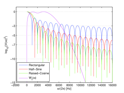
Figure 1: Examples of time–limited shaping filters commonly used in the literature (frequency responses). The time responses are as follows. i) Rectangular pulse: $v\left(\xi\right)=p_{T_{0}}\left(\xi\right)$, where $p_{T_{0}}\left(\xi\right)=1$ if $-T_{0}/2\leq\xi\leq T_{0}/2$ and $p_{T_{0}}\left(\xi\right)=1$ elsewhere. ii) Half–sine pulse: $v\left(\xi\right)=\sqrt{2}\sin\left[{\pi\left({\xi+0.5T_{0}}\right)/T_{0}}\right]p_{T_{0}}\left(\xi\right)$. iii) Raised–cosine pulse: $v\left(\xi\right)=\sqrt{2/3}\left\{{1-\cos\left[{2\pi\left({\xi+0.5T_{0}}\right)/T_{0}}\right]}\right\}p_{T_{0}}\left(\xi\right)$. iv) The orthogonal shaping filters for $N_{t}=4$ are given in (35) in Appendix A with $t_{0}=10^{-4}$. $T_{0}=10^{-3}$ is the time duration of the filters. The frequency response is defined as $V\left(\omega\right)=\left(1/{\sqrt{2\pi}}\right)\int\nolimits_{-\infty}^{+\infty}{v\left(\xi\right)\exp\left({-j\omega\xi}\right)d\xi}$. They are as follows. i) Rectangular pulse: $\left|{V\left({2\pi\omega}\right)}\right|=\kappa_{r}{\rm{sinc}}\left({\omega T_{0}}\right)$, where ${\rm{sinc}}\left(x\right)=1$ if $x=0$ and ${\rm{sinc}}\left(x\right)=\sin\left({\pi x}\right)/\pi x$ if $x\neq 0$. ii) Half–sine pulse: $\left|{V\left({2\pi\omega}\right)}\right|=\kappa_{hs}\left[{\cos\left({\pi\omega T_{0}}\right)/\left({1-4\omega^{2}T_{0}^{2}}\right)}\right]$. iii) Raised–cosine pulse: $\left|{V\left({2\pi\omega}\right)}\right|=\kappa_{rc}\left[{{\rm{sinc}}\left({\omega T_{0}}\right)+\left({1/2}\right){\rm{sinc}}\left({\omega T_{0}-1}\right)+\left({1/2}\right){\rm{sinc}}\left({\omega T_{0}+1}\right)}\right]$. iv) The orthogonal shaping filters for $N_{t}=4$ are given in (36) in Appendix A with $t_{0}=10^{-4}$. $\kappa_{r}$, $\kappa_{hs}$, and $\kappa_{rc}$ are constant factors that are not relevant for our analysis.

Let us now compare the bandwidth efficiency of the orthogonal shaping filters available in Appendix A with state–of–the–art shaping filters. A qualitative and quantitative comparisons are shown in Fig. 1 and in Table I, respectively, by using two commonly adopted definitions of bandwidth [48]: i) the Fractional Power Containment Bandwidth (FPCB) [48, p. 15]; and ii) the Bounded Power Spectral Density Bandwidth (BPSDB) [48, p. 18]. The formal definition of these two concepts of bandwidth is given in the caption of Table I. By carefully analyzing both Table I and Fig. 1, we notice that the bandwidth efficiency of the different shaping filters depend on how stringent the criterion to define the bandwidth is. In particular, if the percentage of energy that is required to be contained in the bandwidth (FPCB) is 99%, then the best shaping filter to use is the half–sine. On the other hand, if, to reduce the interference produced in adjacent transmission bands, the requirement moves from 99% to 99.99999%, then the best shaping filters to us are those given in Appendix A. A similar comment applies when the BPSDB definition of bandwidth is used, but the best shaping filters are the raised–cosine (less stringent requirement) and the orthogonal filters in Appendix A (more stringent requirement). A similar trade–off has been shown in [40] and [48] for conventional modulation schemes and shaping filters.

In other words, the shaping filters in Appendix A are designed to have a very flat spectrum in the transmission band to improve the energy efficiency, as well as a very fast roll–off to reduce interference and enhance coexistence capabilities. This is especially useful to increase the system efficiency since current standards require the transmitted spectrum to occupy a well–defined spectral mask, e.g., for Wireless Local Area Networks (WLAN) and UWB wireless systems. For this reason, the shaping filters in Appendix A have a very good energy containment and bounded energy spectrum. Finally, we emphasize that the shaping filters given in Appendix A are just an example of time–orthogonal filters that can be obtained with state–of–the–art signal processing algorithms [46], [47], as well as that the waveforms compared in Table I have the same time–duration $T_{m}$, and, thus, they provide the same signaling rate $1/T_{m}$.

For illustrative purposes, in this paper we choose the shaping filters with the main objective to limit, as much as possible, out–of–band interference in order to enhance the coexistence capabilities of our communication system, and to reduce interference in adjacent transmission bands. Thus, our criterion is based on choosing filters which, for the same time–duration, have a stringent energy containment or bounded energy spectrum. For example, we assume either ${{\rm{X}}_{\rm{\%}}}>99.9999\%$ or ${{\rm{TH}}_{{\rm{dB}}}}>6{{\rm{dB}}}$ in Table I. With these assumptions, the orthogonal shaping filters given in Appendix A are the best choice, and are chosen to obtain the simulation results in Section VI. For applications where less stringent coexistence capabilities might be required, the shaping filters given in Appendix A might not be the best choice, as they would require a larger bandwidth. In that case, by using the algorithms in [25], [46], [47], and references therein, new orthogonal pulses could be generated with the required time–duration and (practical) bandwidth.

VI Numerical and Simulation Results

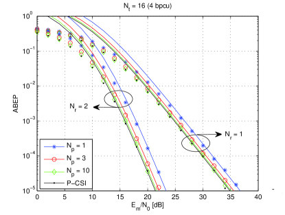
Figure 8: ABEP of TOSD–SSK modulation against $E_{m}/N_{0}$ for: i) $N_{t}=16$ (4 bpcu); ii) $N_{r}=\left\{{1,2}\right\}$; iii) $N_{p}=\left\{{1,3,10}\right\}$; and iv) P–CSI denotes the ABEP with no channel estimation errors. Solid lines show the analytical model and markers show Monte Carlo simulations.

In this section, we show some numerical examples in order to: i) study the performance of SSK and TOSD–SSK modulations in the presence of channel estimation errors; ii) compare the achievable performance with single–antenna and Alamouti schemes; and iii) assess the accuracy of our analytical derivation. For illustrative purposes, i.i.d Rayleigh fading channels are considered in all the analyzed scenarios. The interested reader might find in [7], [11], and [18] numerical examples about the performance of SSK and TOSD–SSK modulations for different wireless channels. Single–antenna and Alamouti schemes are chosen as state–of–the–art transmission technologies for performance comparison because they have the same diversity order and the same decoding complexity as SSK and TOSD–SSK modulations, respectively. The interested reader might find in [49, Fig. 2] the comparison with transmit–diversity Space–Time–Block–Codes (STBCs) for MIMO systems with more than two antennas at the transmitter, and in [50, Fig. 8] the comparison with spatial multiplexing MIMO systems with multi–user detection. In these latter cases, both STBCs and spatial multiplexing MIMO have higher decoding complexity and worse performance than space modulation.

The simulation setup used in our study is as follows: i) we consider i.i.d Rayleigh fading with unit–power over all the wireless links. The related analytical framework is available, by setting $\Omega_{0}=1$, in (20) and (34) for SSK and TOSD–SSK modulations, respectively; ii) $r_{pm}=1$ for all the analyzed scenarios; iii) the bpcu of SSK and TOSD–SSK modulations are equal to $R=\log_{2}\left({N_{t}}\right)$; iv) as far single–antenna and Alamouti schemes are concerned, we consider QAM with constellation size $M$ and bpcu equal to $R=\log_{2}\left({M}\right)$; v) as mentioned in Section V, the shaping filters are obtained from [25]. For example, when $N_{t}=4$, $w_{t_{1}}\left(\cdot\right)$ in Appendix A is used for SSK modulation, single–antenna, and Alamouti schemes, while the set of four orthogonal filters in (35) is used for TOSD–SSK modulation. Furthermore, for a fair comparison among the modulation schemes, the same spectral efficiency (measured in bpcu) is considered; vi) the ABEP of the P–CSI scenario is computed by assuming an infinite number of pilot pulses; vii) the ABEP of single–antenna and Alamouti schemes is obtained through Monte Carlo simulations only, but to check that our simulator is well–tuned the numerical results are compared, for the P–CSI scenario, to the ABEP predicted by the union–bound recently developed in [50] for single– and multi–user systems; viii) as far as single–antenna schemes are concerned, $E_{m}$ is the average energy transmitted for each information symbol; and ix) as far as the Alamouti scheme is concerned, $E_{m}$ is the average energy transmitted for each information symbol from the two active transmit–antennas, i.e., $E_{m}$ is equally split between the two antennas.

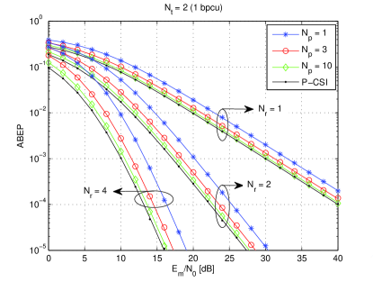
Figure 2: ABEP of SSK modulation against $E_{m}/N_{0}$ for: i) $N_{t}=2$ (1 bpcu); ii) $N_{r}=\left\{{1,2,4}\right\}$; iii) $N_{p}=\left\{{1,3,10}\right\}$; and iv) P–CSI denotes the ABEP with no channel estimation errors. Solid lines show the analytical model and markers show Monte Carlo simulations.

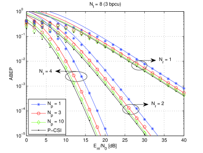
Figure 3: ABEP of SSK modulation against $E_{m}/N_{0}$ for: i) $N_{t}=8$ (3 bpcu); ii) $N_{r}=\left\{{1,2,4}\right\}$; iii) $N_{p}=\left\{{1,3,10}\right\}$; and iv) P–CSI denotes the ABEP with no channel estimation errors. Solid lines show the analytical model and markers show Monte Carlo simulations.

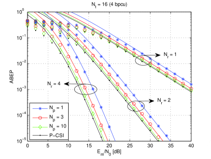
Figure 4: ABEP of SSK modulation against $E_{m}/N_{0}$ for: i) $N_{t}=16$ (4 bpcu); ii) $N_{r}=\left\{{1,2,4}\right\}$; iii) $N_{p}=\left\{{1,3,10}\right\}$; and iv) P–CSI denotes the ABEP with no channel estimation errors. Solid lines show the analytical model and markers show Monte Carlo simulations.

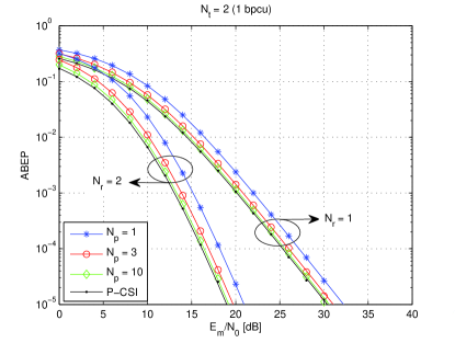
Figure 7: ABEP of TOSD–SSK modulation against $E_{m}/N_{0}$ for: i) $N_{t}=2$ (1 bpcu); ii) $N_{r}=\left\{{1,2}\right\}$; iii) $N_{p}=\left\{{1,3,10}\right\}$; and iv) P–CSI denotes the ABEP with no channel estimation errors. Solid lines show the analytical model and markers show Monte Carlo simulations.

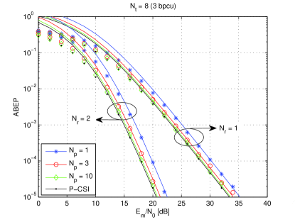
Figure 9: ABEP of TOSD–SSK modulation against $E_{m}/N_{0}$ for: i) $N_{t}=8$ (3 bpcu); ii) $N_{r}=\left\{{1,2}\right\}$; iii) $N_{p}=\left\{{1,3,10}\right\}$; and iv) P–CSI denotes the ABEP with no channel estimation errors. Solid lines show the analytical model and markers show Monte Carlo simulations.

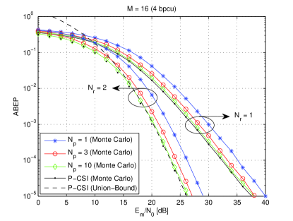
Figure 10: ABEP of Alamouti scheme with QAM against $E_{m}/N_{0}$ for: i) $M=16$ (4 bpcu); ii) $N_{r}=\left\{{1,2}\right\}$; iii) $N_{p}=\left\{{1,3,10}\right\}$; and iv) P–CSI denotes the ABEP with no channel estimation errors. Solid lines with markers or just markers show Monte Carlo simulations. Dashed lines show the union–bound computed from [50] with no channel estimation errors at the receiver (P–CSI scenario). This union–bound is shown only for a subset of curves in order to improve the readability of the figure, and avoid overlap among closely–spaced curves.

The results are shown in Figs. 2–6 for transmission technologies with no transmit–diversity gain (SSK and QAM), and in Figs. 7–10 for transmission technologies with transmit–diversity gain (TOSD–SSK and Alamouti). As far as SSK and TOSD–SSK modulations are concerned, we observe that: i) our analytical frameworks are very accurate and asymptotically–tight for all the analyzed scenarios. In particular, as expected, they are exact for $N_{t}=2$; ii) there is no loss of the diversity order in the presence of channel estimation errors. Only a loss of the coding gain can be observed for all MIMO setups; iii) even though in space modulation the information is encoded into the CIRs, the performance degradation observed when reducing the number of pilot pulses, $N_{p}$, is not very high, and the ABEP is very close to the P–CSI lower–bound, in the analyzed scenarios, for $N_{p}=10$; iv) SSK and TOSD–SSK modulations have a SNR penalty, with respect to the P–CSI lower–bound, of approximately 3dB and 2dB when $N_{p}=1$, respectively; v) the ABEP gets worse for increasing $N_{t}$, as a consequence of the increased size of the spatial–constellation diagram, and gets better for increasing $N_{r}$, due to the receive–diversity gain; and vi) TOSD–SSK modulation significantly outperforms SSK modulation, due to the transmit–diversity gain introduced by the orthogonal pulse shaping design.

As far as the performance comparison with single–antenna and Alamouti schemes is concerned, the following conclusions can be drawn (see Table II for numerical values): i) SSK modulation outperforms single–antenna QAM, in all the analyzed scenarios, for spectral efficiencies greater than 2 bpcu and for $N_{r}>1$. If $N_{r}=1$, QAM always outperforms SSK modulation; ii) SSK and single–antenna QAM have almost the same robustness to channel estimation errors, with a SNR penalty, with respect to the P–CSI lower–bound, of approximately 3dB when $N_{p}=1$; iii) TOSD–SSK modulation outperforms the Alamouti scheme with QAM, in all the analyzed scenarios, for spectral efficiencies greater than 2 bpcu. In particular, unlike SSK modulation, TOSD–SSK modulation is superior to the Alamouti scheme with QAM for $N_{r}=1$ as well. This is due to the transmit–diversity gain of TOSD–SSK modulation; iv) TOSD–SSK modulation is more robust to channel estimation errors than the Alamouti scheme with QAM. A clear example can be observed in Table II when $R=2$ bpcu and $N_{p}=1$. In fact, the Alamouti scheme is superior to TOSD–SSK modulation in the P–CSI scenario, but TOSD–SSK modulation provides better performance if $N_{p}=1$ and $N_{r}>1$. More in general, Table II shows that the Alamouti scheme with QAM has a SNR penalty, with respect to the P–CSI lower–bound, of approximately 3dB when $N_{p}=1$, while TOSD–SSK modulation has a SNR penalty of only 2dB; and v) the performance gain of SSK and TOSD–SSK modulations with respect to single–antenna and Alamouti schemes increases with $N_{r}$, because, as analytically proved in [50], space modulation takes much better advantage of receive–diversity. The results shown in this section confirm that this trend is retained in the presence of channel estimation errors as well.

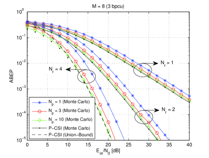
Figure 5: ABEP of QAM against $E_{m}/N_{0}$ for: i) $M=8$ (3 bpcu); ii) $N_{r}=\left\{{1,2,4}\right\}$; iii) $N_{p}=\left\{{1,3,10}\right\}$; and iv) P–CSI denotes the ABEP with no channel estimation errors. Solid lines with markers or just markers show Monte Carlo simulations. Dashed lines show the union–bound computed from [50] with no channel estimation errors at the receiver (P–CSI scenario). This union–bound is shown only for a subset of curves in order to improve the readability of the figure, and avoid overlap among closely–spaced curves.

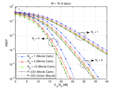
Figure 6: ABEP of QAM against $E_{m}/N_{0}$ for: i) $M=16$ (4 bpcu); ii) $N_{r}=\left\{{1,2,4}\right\}$; iii) $N_{p}=\left\{{1,3,10}\right\}$; and iv) P–CSI denotes the ABEP with no channel estimation errors. Solid lines with markers or just markers show Monte Carlo simulations. Dashed lines show the union–bound computed from [50] with no channel estimation errors at the receiver (P–CSI scenario). This union–bound is shown only for a subset of curves in order to improve the readability of the figure, and avoid overlap among closely–spaced curves.

In conclusion, SSK modulation is as robust as single–antenna systems to imperfect channel knowledge, and it provides better performance when the target spectral efficiency is greater than 2 bpcu and $N_{r}>1$. On the other hand, TOSD–SSK modulation is more robust than the Alamouti scheme to imperfect channel knowledge, and it provides better performance when the target spectral efficiency is greater than 2 bpcu. In all the cases, the price to be paid for this performance improvement is the need of increasing the number of radiating elements $N_{t}$ at the transmitter, while still retaining a single–RF chain and avoiding inter–antenna synchronization, which are beneficial for low–complexity implementations [42]. This remark is somehow similar to [51], as far as the achievable transmit–diversity of STBCs is concerned. Finally, it is worth emphasizing that the need of a large number of radiating elements seems not to be a critical bottleneck for the development of the next generation cellular systems, as current research is moving towards the utilization of the millimeter–wave frequency spectrum [52]. In fact, in this band compact horn antenna–arrays with 48 elements and compact patch antenna–arrays with more than 4 elements at the base station and at the mobile terminal, respectively, are currently being developed to support multi–gigabit transmission rates [53]. Furthermore, SSK and TOSD–SSK seem to be well–suited low–complexity modulation schemes for the recently proposed “massive MIMO” paradigm [54], according to which unprecedent spectral efficiencies can be achieved in cellular networks by using antenna–arrays with very large (with tens or hundreds) active radiating elements.

VII Conclusion

In this paper, we have analyzed the performance of space modulation when CSI is not perfectly known at the receiver. A very accurate and general analytical framework has been proposed, and it has been shown that, unlike common belief, SSK modulation has the same robustness to channel estimation errors as conventional modulation schemes, while TOSD–SSK modulation is less sensitive to channel estimation errors than conventional modulations. Also, it has been shown that few pilot pulses are needed to achieve almost the same performance as the P–CSI lower–bound, and that the performance gain, over state–of–the–art MIMO technologies, promised by space modulation is retained even with imperfect channel knowledge. These results confirm the usefulness of space modulation in practical operating conditions, and, in particular, the notable performance advantage of TOSD–SSK modulation, which provides transmit–diversity and is more robust to channel estimation errors than conventional schemes, such as the Alamouti code.

Appendix A Orthogonal Shaping Filters for $N_{t}=4$

In this appendix, we show an example of orthogonal shaping filters that can be used for TOSD–SSK modulation. Without loss of generality we consider the case study with $N_{t}=4$, but the procedure can be generalized to larger antenna–arrays.

More specifically, we consider the procedure described in [25], which allows us to generate orthogonal shaping filters with the same time–duration and bandwidth. Similar techniques are available in [46], [47]. From [25], we can obtain the four orthogonal impulse (time) responses shown in (35) at the bottom of the previous page, as well as the four related frequency responses (Fourier transform) $P\left(\omega\right)=\left({{1\mathord{\left/{\vphantom{1{\sqrt{2\pi}}}}\right.\kern-1.2pt}{\sqrt{2\pi}}}}\right)\int\nolimits_{-\infty}^{+\infty}{p\left(\xi\right)\exp\left({-j\omega\xi}\right)d\xi}$ shown in (36) at the bottom of the previous page too, where we have defined:

$$\left\{\begin{array}[]{l}p_{1}\left(\xi\right)=\left({\frac{1}{{\sqrt{\sqrt{\pi}}}}}\right)\exp\left[{-\frac{1}{2}\left({\frac{\xi}{{t_{0}}}}\right)^{2}}\right]\\ p_{2}\left(\xi\right)=\left({\frac{{2\xi}}{{\sqrt{2\sqrt{\pi}}}}}\right)\exp\left[{-\frac{1}{2}\left({\frac{\xi}{{t_{0}}}}\right)^{2}}\right]\\ p_{3}\left(\xi\right)=\left({\frac{{4\xi^{2}-2}}{{\sqrt{8\sqrt{\pi}}}}}\right)\exp\left[{-\frac{1}{2}\left({\frac{\xi}{{t_{0}}}}\right)^{2}}\right]\\ p_{4}\left(\xi\right)=\left({\frac{{8\xi^{3}-12\xi}}{{\sqrt{48\sqrt{\pi}}}}}\right)\exp\left[{-\frac{1}{2}\left({\frac{\xi}{{t_{0}}}}\right)^{2}}\right]\\ p_{5}\left(\xi\right)=\left({\frac{{16\xi^{4}-48\xi^{2}+12}}{{\sqrt{384\sqrt{\pi}}}}}\right)\exp\left[{-\frac{1}{2}\left({\frac{\xi}{{t_{0}}}}\right)^{2}}\right]\\ \end{array}\right.$$ (37)

and:

$$\left\{\begin{array}[]{l}P_{1}\left(\omega\right)=\left({\frac{{t_{0}}}{{\sqrt{\sqrt{\pi}}}}}\right)\exp\left[{-\frac{1}{2}\left({t_{0}\omega}\right)^{2}}\right]\\ P_{2}\left(\omega\right)=\left({\frac{{2jt_{0}^{2}\omega}}{{\sqrt{2\sqrt{\pi}}}}}\right)\exp\left[{-\frac{1}{2}\left({t_{0}\omega}\right)^{2}}\right]\\ P_{3}\left(\omega\right)=\left({\frac{{2t_{0}-4t_{0}^{3}\omega^{2}}}{{\sqrt{8\sqrt{\pi}}}}}\right)\exp\left[{-\frac{1}{2}\left({t_{0}\omega}\right)^{2}}\right]\\ P_{4}\left(\omega\right)=\left({\frac{{12jt_{0}^{2}\omega-8jt_{0}^{4}\omega^{3}}}{{\sqrt{48\sqrt{\pi}}}}}\right)\exp\left[{-\frac{1}{2}\left({t_{0}\omega}\right)^{2}}\right]\\ P_{5}\left(\omega\right)=\left({\frac{{12t_{0}-48t_{0}^{3}\omega^{2}+16t_{0}^{5}\omega^{4}}}{{\sqrt{384\sqrt{\pi}}}}}\right)\exp\left[{-\frac{1}{2}\left({t_{0}\omega}\right)^{2}}\right]\\ \end{array}\right.$$ (38)

Finally, we mention that, by adjusting the form factor $t_{0}$, the bandwidth can be arbitrarily chosen, and both narrow– and wide–band communication systems can be considered.

Marco Di Renzo (SM’05–AM’07–M’09) was born in L’Aquila, Italy, in 1978. He received the Laurea (cum laude) and the Ph.D. degrees in Electrical and Information Engineering from the Department of Electrical and Information Engineering, University of L’Aquila, Italy, in April 2003 and in January 2007, respectively. From August 2002 to January 2008, he was with the Center of Excellence for Research DEWS, University of L’Aquila, Italy. From February 2008 to April 2009, he was a Research Associate with the Telecommunications Technological Center of Catalonia (CTTC), Barcelona, Spain. From May 2009 to December 2009, he was an EPSRC Research Fellow with the Institute for Digital Communications (IDCOM), The University of Edinburgh, Edinburgh, United Kingdom (UK). Since January 2010, he has been a Tenured Researcher (“Chargé de Recherche Titulaire”) with the French National Center for Scientific Research (CNRS), as well as a research staff member of the Laboratory of Signals and Systems (L2S), a joint research laboratory of the CNRS, the École Supérieure d’Électricité (SUPÉLEC), and the University of Paris–Sud XI, Paris, France. His main research interests are in the area of wireless communications theory, signal processing, and information theory. Dr. Di Renzo is the recipient of the special mention for the outstanding five–year (1997–2003) academic career, University of L’Aquila, Italy; the THALES Communications fellowship for doctoral studies (2003–2006), University of L’Aquila, Italy; and the Torres Quevedo award for his research on ultra wide band systems and cooperative localization for wireless networks (2008–2009), Ministry of Science and Innovation, Spain.

Dario De Leonardis was born in Atri, Italy, in 1984. He received the Bachelor and the Master degrees in Telecommunications Engineering from the Department of Electrical and Information Engineering, University of L’Aquila, Italy, in October 2006 and in May 2009, respectively. From September 2008 to March 2009, he was a Visiting ERASMUS student at the Telecommunications Technological Center of Catalonia (CTTC), Barcelona, Spain, where he conducted research for his Master thesis project on low–complexity receiver design for ultra wide band wireless systems. In April 2010, he received a personal research grant from the National Inter–University Consortium for Telecommunications (CNIT), Italy, to conduct research on space modulation for multiple–input–multiple–output wireless systems, and he was affiliated with the Department of Electrical and Information Engineering and the Center of Excellence for Research DEWS, University of L’Aquila, Italy. Since December 2010, he has been a Ph.D. candidate in the same institution. His main research interests are in the area of wireless communications.

Fabio Graziosi (S’96 -M’97) was born in L’Aquila, Italy, in 1968. He received the Laurea degree (cum laude) and the Ph.D. degree in electronic engineering from the University of L’Aquila, Italy, in 1993 and in 1997, respectively. Since February 1997, he has been with the Department of Electrical Engineering, University of L’Aquila, where he is currently an Associate Professor. He is a member of the Executive Committee, Center of Excellence Design methodologies for Embedded controllers, Wireless interconnect and System-on-chip (DEWS), University of L’Aquila, and the Executive Committee, Consorzio Nazionale Interuniversitario per le Telecomunicazioni (CNIT). He is also the Chairman of the Board of Directors of WEST Aquila s.r.l., a spin–off R&D company of the University of L’Aquila, and the Center of Excellence DEWS. He is involved in major national and European research programs in the field of wireless systems and he has been a reviewer for major technical journals and international conferences in communications. He also serves as Technical Program Committee (TPC) member and Session Chairman of several international conferences in communications. His current research interests are mainly focused on wireless communication systems with emphasis on wireless sensor networks, ultra wide band communication techniques, cognitive radio, and cooperative communications.

Harald Haas (SM’98–AM’00–M’03) holds the Chair of Mobile Communications in the Institute for Digital Communications (IDCOM) at the University of Edinburgh. His main research interests are in the areas of wireless system design and analysis as well as digital signal processing, with a particular focus on interference coordination in wireless networks, spatial modulation and optical wireless communication. Professor Haas holds more than 15 patents. He has published more than 50 journal papers including a Science Article and more than 140 peer–reviewed conference papers. Nine of his papers are invited papers. He has co–authored a book entitled “Next Generation Mobile Access Technologies: Implementing TDD” with Cambridge University Press. Since 2007, he has been a Regular High Level Visiting Scientist supported by the Chinese “111 program” at Beijing University of Posts and Telecommunications (BUPT). He was an invited speaker at the TED Global conference 2011. He has been shortlisted for the World Technology Award for communications technology (individual) 2011.

References

- [1] M. Di Renzo, H. Haas, and P. M. Grant, “Spatial modulation for multiple–antenna wireless systems: A survey”, IEEE Commun. Mag., vol. 49, no. 12, pp. 182–191, Dec. 2011.
- [2] Y. Yang and B. Jiao, “Information–guided channel–hopping for high data rate wireless communication”, IEEE Commun. Lett., vol. 12, no. 4, pp. 225–227, Apr. 2008.
- [3] R. Y. Mesleh, H. Haas, S. Sinanovic, C. W. Ahn, and S. Yun, “Spatial modulation”, IEEE Trans. Veh. Technol., vol. 57, no. 4, pp. 2228–2241, July 2008.
- [4] J. Jeganathan, A. Ghrayeb, L. Szczecinski, and A. Ceron, “Space shift keying modulation for MIMO channels”, IEEE Trans. Wireless Commun., vol. 8, no. 7, pp. 3692–3703, July 2009.
- [5] N. Serafimovski, M. Di Renzo, S. Sinanovic, R. Y. Mesleh, and H. Haas, “Fractional bit encoded spatial modulation (FBE–SM)”, IEEE Commun. Lett., vol. 14, no. 5, pp. 429–431, May 2010.
- [6] M. Di Renzo and H. Haas, “Improving the performance of space shift keying (SSK) modulation via opportunistic power allocation”, IEEE Commun. Lett., vol. 14, no. 6, pp. 500–502, June 2010.
- [7] M. Di Renzo and H. Haas, “A general framework for performance analysis of space shift keying (SSK) modulation for MISO correlated Nakagami–m fading channels”, IEEE Trans. Commun., vol. 58, no. 9, pp. 2590–2603, Sep. 2010.
- [8] M. Di Renzo and H. Haas, “Performance comparison of different spatial modulation schemes in correlated fading channels”, IEEE Int. Conf. Commun., pp. 1–6, May 2010.
- [9] E. Basar, U. Aygolu, E. Panayirci, and H. V. Poor, “Space–time block coded spatial modulation”, IEEE Trans. Commun., vol. 59, no. 3, pp. 823–832, Mar. 2011.
- [10] S. Sugiura, S. Chen, and L. Hanzo, “Coherent and differential space–time shift keying: A dispersion matrix approach”, IEEE Trans. Commun., vol. 58, no. 11, pp. 3219–3230, Nov. 2010.
- [11] M. Di Renzo and H. Haas, “Space shift keying (SSK–) MIMO over correlated Rician fading channels: Performance analysis and a new method for transmit–diversity”, IEEE Trans. Commun., vol. 59, no. 1, pp. 116–129, Jan. 2011.
- [12] S. Sugiura, S. Chen, and L. Hanzo, “A unified MIMO architecture subsuming space shift keying, OSTBC, BLAST and LDC”, IEEE Veh. Technol. Conf. – Fall, pp. 1–5, Sep. 2010.
- [13] J. Jeganathan, A. Ghrayeb, and L. Szczecinski, “Spatial modulation: Optimal detection and performance analysis”, IEEE Commun. Lett., vol. 12, no. 8, pp. 545–547, Aug. 2008.
- [14] J. Jeganathan, A. Ghrayeb, and L. Szczecinski, “Generalized space shift keying modulation for MIMO channels”, IEEE Int. Symp. Personal, Indoor, Mobile Radio Commun., pp. 1–5, Sep. 2008.
- [15] T. Handte, A. Muller, and J. Speidel, “BER analysis and optimization of generalized spatial modulation in correlated fading channels”, IEEE Veh. Technol. Conf. – Fall, pp. 1–5, Sep. 2009.
- [16] R. Y. Mesleh, M. Di Renzo, H. Haas, and P. M. Grant, “Trellis coded spatial modulation”, IEEE Trans. Wireless Commun., vol. 9, no. 7, pp. 2349–2361, July 2010.
- [17] M. Di Renzo and H. Haas, “Performance analysis of spatial modulation”, IEEE Int. Conf. Commun. Networking in China, pp. 1–7, Aug. 2010.
- [18] M. Di Renzo and H. Haas, “Space shift keying (SSK) modulation with partial channel state information: Optimal detector and performance analysis over fading channels”, IEEE Trans. Commun., vol. 58, no. 11, pp. 3196–3210, Nov. 2010.
- [19] M. M. Ulla Faiz, S. Al–Ghadhban, and A. Zerguine, “Recursive least–squares adaptive channel estimation for spatial modulation systems”, IEEE Malaysia Int. Conf. Commun., pp. 1–4, Dec. 2009.
- [20] P. Wolniansky, G. Foschini, G. Golden, and R. Valenzuela, “V–BLAST: An architecture for realizing very high data rates over the rich–scattering wireless channel”, IEEE Int. Symp. Signals, Systems, Electr., pp. 295–300, Sep./Oct. 1998.
- [21] S. M. Alamouti, “A simple transmit diversity technique for wireless communications”, IEEE J. Sel. Areas Commun., vol. 16, no. 8, pp. 1451–1458, Oct. 1998.
- [22] G. Taricco and E. Biglieri, “Space–time decoding with imperfect channel estimation”, IEEE Trans. Wireless Commun., vol. 4, no. 4, pp. 1874–1888, July 2005.
- [23] M. Di Renzo F. Graziosi, and F. Santucci, “On the cumulative distribution function of quadratic–form receivers over generalized fading channels with tone interference”, IEEE Trans. Commun., vol. 57, no. 7, pp. 2122–2137, July 2009.
- [24] M. Di Renzo and H. Haas, “Space shift keying (SSK) modulation: On the transmit–diversity/multiplexing trade–off”, IEEE Int. Conf. Commun., pp. 1–6, June 2011.
- [25] J. A. Ney da Silva and M. L. R. de Campos, “Spectrally efficient UWB pulse shaping with application in orthogonal PSM”, IEEE Trans. Commun., vol. 55, no. 2, pp. 313–322, Feb. 2007.
- [26] R. Derryberry, S. Gray, D. Ionescu, G. Mandyam, and B. Raghothaman, “Transmit diversity in 3G CDMA systems”, IEEE Commun. Mag., vol. 40, vol. 4, pp. 68-75, Apr. 2002.
- [27] J. G. Proakis, “Probabilities of error for adaptive reception of M–phase signals”, IEEE Trans. Commun. Technol., vol. COM–16, no. 1, pp. 71–81, Feb. 1968.
- [28] W. M. Gifford, M. Z. Win, and M. Chiani, “Diversity with practical channel estimation”, IEEE Trans. Wireless Commun., vol. 4, no. 4, pp. 1935–1947, July 2005.
- [29] M. K. Simon and M.–S. Alouini, Digital Communication over Fading Channels, John Wiley Sons, Inc., 1st ed., 2000.
- [30] H. L. Van Trees, Detection, Estimation, and Modulation Theory, Part I: Detection, Estimation, and Linear Modulation Theory, John Wiley Sons, Inc. 2001.
- [31] M. I. Irshid and I. Salous, “Bit error probability for coherent M–ary PSK systems” IEEE Trans. Commun., vol. 39, no. 3, pp. 349–352, Mar. 1991.
- [32] J. G. Proakis, “On the probability of error for multichannel reception of binary signals”, IEEE Trans. Commun. Technol., vol. COM–16, no. 1, pp. 68–71, Feb. 1968.
- [33] M. K. Simon and M.–S. Alouini, “A unified approach to the probability of error for noncoherent and differentially coherent modulations over generalized fading channels”, IEEE Trans. Commun., vol. 46, no. 12, pp. 1625–1638, Dec. 1998.
- [34] L.–F. Tsaur and D. C. Lee, “Simplifying performance expressions for noncoherent and differentially coherent modulations over generalized fading multiple channels”, IEEE Trans. Commun., vol. 49, no. 4, pp. 583–584, Apr. 2001.
- [35] C. O’Driscoll and C. C. Murphy, “A simplified expression for the probability of error for binary multichannel communications”, IEEE Trans. Commun., vol. 57, no. 1, pp. 32–35, Jan. 2009.
- [36] M. K. Simon, Probability Distributions Involving Gaussian Random Variables: A Handbook for Engineers and Scientists, Kluwer, 2002.
- [37] J. Gil–Pelaez, “Note on the inversion theorem” Biometrika, vol. 38, pp. 481–482, Dec. 1951.
- [38] M. Di Renzo and H. Haas, “Bit error probability of space modulation over Nakagami–m fading: Asymptotic analysis”, IEEE Commun. Lett., vol. 15, no. 10, pp. 1026–1028, Oct. 2011.
- [39] Z. Wang and G. B. Giannakis, “A simple and general parameterization quantifying performance in fading channels”, IEEE Trans. Commun., vol. 51, no. 8, pp. 1389–1398, Aug. 2003.
- [40] H. Wei, L.–L. Yang, and L. Hanzo, “On the performance of band–limited asynchronous DS–CDMA over Nakagami–m channels”, IEEE Trans. Wireless Commun., vol. 5, no. 7, pp. 1586–1593, July 2006.
- [41] A. S. Kang and V. Sharma, “Data communication using pulse shaping techniques in wireless signal processing approach – In depth review”, Int. J. of Computational Engineering and Management, vol. 22, pp. 24–33, Apr. 2011.
- [42] A. Kalis, A. G. Kanatas, and C. B. Papadias, “A novel approach to MIMO transmission using a single RF front end”, IEEE J. Select. Areas Commun., vol. 26, no. 6, pp. 972–980, Aug. 2008.
- [43] O. N. Alrabadi, C. B. Papadias, A. Kalis, and R. Prasad, “A universal encoding scheme for MIMO transmission using a single active element for PSK modulation schemes”, IEEE Trans. Wireless Commun., vol. 8, no. 9, pp. 5133–5143, Sep. 2009.
- [44] O. N. Alrabadi, C. Divarathne, P. Tragas, A. Kalis, N. Marchetti, C. B. Papadias, and R. Prasad, “Spatial multiplexing with a single radio: Proof–of–concept experiments in an indoor environment with a 2.6 GHz prototypes”, IEEE Commun. Lett., vol. 15, no. 2, pp. 178–180, Feb. 2011.
- [45] A. Mohammadi and F. M. Ghannouchi, “Single RF front–end MIMO transceivers”, IEEE Commun. Mag., vol. 49, no. 12, pp. 104–109, Dec. 2011.
- [46] B. Parr, B.–L. Cho, K. Wallace, and Z. Ding, “A novel ultra–wideband pulse design algorithm”, IEEE Commun. Lett., vol. 7, no. 5, pp. 219–221, May 2003.
- [47] X. Wu, Z. Tian, T. N. Davidson, and G. B. Giannakis, “Optimal waveform design for UWB radios”, IEEE Trans. Signal Processing, vol. 54, no. 6, pp. 2009–2021, June 2006.
- [48] F. Amoroso, “The bandwidth of digital data signal”, IEEE Commun. Mag., vol. 18, no. 6, pp. 13–24, Nov. 1980.
- [49] M. Di Renzo and H. Haas, “Transmit–diversity for spatial modulation (SM): Towards the design of high–rate spatially–modulated space–time block codes”, IEEE Int. Conf. Commun., pp. 1–6, June 2011.
- [50] M. Di Renzo and H. Haas, “Bit error probability of space shift keying MIMO over multiple–access independent fading channels”, IEEE Trans. Veh. Technol., vol. 60, no. 8, pp. 3694–3711, Oct. 2011.
- [51] V. Tarokh, H. Jafarkhani, and A. R. Calderbank, “Space–time block coding for wireless communications: Performance results”, IEEE J. Sel. Areas Commun., vol. 17, no. 3, pp. 451–460, Mar. 1999.
- [52] F. Khan and J. Pi, “Millimeter–wave mobile broadband: Unleashing 3–300GHz spectrum”, IEEE Wireless Commun. Netw. Conf., Mar. 2011, tutorial presentation. [Online]. Available: http://www.ieee-wcnc.org/2011/tut/t1.pdf.
- [53] S. Rajagopal, S. Abu–Surra, Z. Pi, and F. Khan, “Antenna array design for multi–Gbps mmWave mobile broadband communication”, IEEE Global Commun. Conf., pp. 1–6, Dec. 2011.
- [54] T. L. Marzetta, “Noncooperative cellular wireless with unlimited numbers of base station antennas”, IEEE Trans. Wireless Commun., vol. 9, no. 11, pp. 3590–3600, Nov. 2010.