PageRank and rank-reversal dependence on the damping factor

Abstract

PageRank (PR) is an algorithm originally developed by Google to evaluate the importance of web pages. Considering how deeply rooted Google’s PR algorithm is to gathering relevant information or to the success of modern businesses, the question of rank-stability and choice of the damping factor (a parameter in the algorithm) is clearly important. We investigate PR as a function of the damping factor $d$ on a network obtained from a domain of the World Wide Web, finding that rank-reversal happens frequently over a broad range of PR (and of $d$). We use three different correlation measures, Pearson, Spearman, and Kendall, to study rank-reversal as $d$ changes, and show that the correlation of PR vectors drops rapidly as $d$ changes from its frequently cited value, $d_{0}=0.85$. Rank-reversal is also observed by measuring the Spearman and Kendall rank correlation, which evaluate relative ranks rather than absolute PR. Rank-reversal happens not only in directed networks containing rank-sinks but also in a single strongly connected component, which by definition does not contain any sinks. We relate rank-reversals to rank-pockets and bottlenecks in the directed network structure. For the network studied, the relative rank is more stable by our measures around $d=0.65$ than at $d=d_{0}$.

1 Introduction

Web pages and their hyperlinks comprising the World Wide Web (WWW) can be represented as sets of nodes (vertices) and directed links (edges). Such representations are referred to as complex networks or graphs [1]. Recently, much study has been devoted to dynamics on complex networks in relation to, for example, the spread of epidemics through human travel networks [2], the propagation of viruses through the Internet [3], information diffusion or consensus of opinion in social acquaintance networks [4, 5, 6], and energy or metabolite flux in ecological and metabolic networks [7]. In addition, applications of network dynamics have been explored as powerful predictive mechanisms for elucidating community structure [8, 9] and node centrality [10]. Foremost among these various applications is Google’s ranking algorithm [11], PageRank (PR), a centrality or importance measure based on random walks.

As originally conceived, PR rates web pages according to a link analysis that takes into consideration only the topological structure of the Web, and not the contents of its pages [11, 12], using a fundamental dynamic process, random walks [13, 14]. The algorithm assumes that a random surfer (walker), starting from a random web page, chooses the next page to which it will move by clicking at random, with probability $d$, one of the hyperlinks in the current page. This probability is represented by a so-called ‘damping factor’ $d$, where $d\in(0,1)$. Otherwise, with probability $(1-d)$, the surfer jumps to any web page in the network. If a page is a dangling end, meaning it has no outgoing hyperlinks, the random surfer selects an arbitrary web page from a uniform distribution and “teleports” to that page. In the case that many random surfers exhibit the same surfing behavior, such that a stationary state exists, the density of the surfers at each page indicates the relative importance of each web page, i.e., its PageRank.

Denoting the total number of pages as $N$, the elements of the transition matrix $\boldsymbol{P}$ are defined such that if page $j$ has an outgoing link to $i$ (here we ignore multiple links), $p_{ij}=1/k^{\rm out}_{j}$, where $k^{\rm out}_{j}$ is the outgoing degree of page $j$, $p_{ij}=1/N$ if page $j$ is a dangling end with no outgoing degree ($k^{\rm out}_{j}=0$), and $p_{ij}=0$, otherwise. We can describe the evolution of the PR (column) vector $\boldsymbol{\pi}$ by the equation

$$\boldsymbol{\pi}(t)=d\boldsymbol{P}\boldsymbol{\pi}(t-1)+\frac{(1-d)}{N}\boldsymbol{1},$$ (1)

where the column vector $\boldsymbol{1}=[1,\ldots,1]^{T}$, $\pi_{i}(t)$ is the probability to be on page $i$ at time $t$, and $d$ is the damping factor. If we write Eq. (1) element-wise,

$$\pi_{i}(t)=d\sum_{j}p_{ij}\pi_{j}(t-1)+\frac{(1-d)}{N}.$$ (2)

For $t\rightarrow\infty$, $\boldsymbol{\pi}(t)$ converges to the stationary state which is given by the solution of the linear system $(\boldsymbol{I}-d\boldsymbol{P})\boldsymbol{\pi}=\frac{(1-d)}{N}\boldsymbol{1}$. Alternatively, PR can be described by $\boldsymbol{\pi}(t)=\boldsymbol{G}\boldsymbol{\pi}(t-1)$ with the Google matrix $\boldsymbol{G}$ defined as

$$\boldsymbol{G}=d\boldsymbol{P}+\frac{(1-d)}{N}\boldsymbol{E},$$ (3)

where the matrix $\boldsymbol{E}=\boldsymbol{1}\boldsymbol{1}^{T}$ is $1$ for all elements. The Google matrix is a Markov matrix. For $d<1$ it is (left) stochastic, aperiodic, and irreducible. The PR vector $\boldsymbol{\pi}$ is the principal eigenvector, i.e., the eigenvector corresponding to the largest eigenvalue 1, of the system $\boldsymbol{G}\boldsymbol{\pi}=\boldsymbol{\pi}$. If $\pi_{i}>\pi_{j}$, then page $i$ ranks above page $j$.

Even though the damping factor $d$ is introduced mainly to prevent the Google matrix from being reducible, its effect on the PR is substantial. When $d$ goes to 0, the random teleport process dominates. The result is a uniform state where all $\pi_{i}=1/N$. On the other hand, as $d$ approaches 1, the transition process dominates, which might suggest that the resulting PR reflects the network structure more accurately. However, the resulting PR is not actually a good indicator for finding important nodes. As Boldi et al. point out, in the limit $d\rightarrow 1$, random walkers trivially concentrate in the rank-sinks [15, 16], nodes (or groups of nodes) which have incoming paths but no outgoing paths. Many important nodes will therefore have zero PR in this limit.

As a result, choosing the damping factor close to 1 does not provide a PR that indicates important nodes. Moreover when the value of $d$ changes, not only can the PR values change significantly [17], but also the relative rankings can be radically altered [18, 19], a process called rank-reversal. When we consider that a top-of-list Google ranking is deeply related to e.g. the success of businesses and sales, rank-reversal stemming from damping factor changes is of more than purely theoretical relevance. Here we investigate rank-reversal dependence on the damping factor and discuss its origin in directed networks.

2 Strongly connected component decomposition

Because hyperlinks are directed, a random surfer may be able to hop from page $A$ to page $B$ (possibly through several hyperlinks), but may find that the return journey (from B to A) is impossible. If this is the case, pages (nodes) $A$ and $B$ are weakly connected. If, however, the surfer can return to $A$ from $B$ along a path of hyperlinks, $A$ and $B$ are considered to be strongly connected. A strongly connected component (SCC) is a maximal subnetwork of a directed network, such that every pair of nodes in it is strongly connected; likewise, a maximal weakly connected subnetwork is a weakly connected component (WCC). A directed network can therefore be naturally decomposed into one or more SCCs without ambiguity. Tarjan’s algorithm [20] efficiently finds the SCCs of a directed network by performing a single depth-first search. If we map each SCC to a virtual node (coarse-graining), a directed network is abstracted as an acyclic weighted network, including self-links, where the size of each virtual node represents the number of nodes contained in its SCC (See Fig. 1).

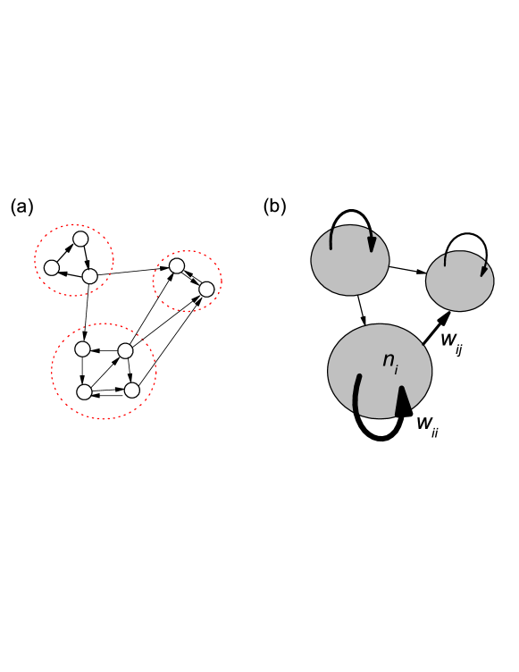
Figure 1: (Color online) SCC diagram. (a) A directed network can be decomposed into several SCCs. Each red-dotted circle in (a) delineates a SCC. (b) A directed network can also be abstracted into a SCC diagram through coarse-graining. This abstracted SCC diagram is an acyclic weighted network, containing self-links (denoted by $w_{ii}$) and size-heterogeneous nodes ($n_{i}$).

The largest SCC is called the giant strongly connected component (GSCC), and every SCC (including single nodes) having paths to the GSCC belongs to an incoming component. Conversely every SCC having paths from the GSCC is called an outgoing component. If a random walker starts from any node in the network of Fig. 1(a) and follows only the directed links without teleporting, the random walker will ultimately be trapped in the top right SCC. This type of “recurrent” SCC is called a rank-sink.

To prevent this situation, the damping factor is used. Nonetheless, depending on one’s choice of $d$, nodes can obtain different ranking. Rank stability refers to how close relative rankings are for different damping factors.

3 Correlation Coefficients

To quantify rank-stability we use three different correlation measures. The first is the well-known Pearson correlation coefficient, which is defined for two paired sequences $(X_{i},Y_{i})$ as follows,

$$r=\frac{\sum_{i=1}^{N}\left(X_{i}-\bar{X}\right)\left(Y_{i}-\bar{Y}\right)}{\sqrt{\sum_{i=1}^{N}\left(X_{i}-\bar{X}\right)^{2}}\sqrt{\sum_{i=1}^{N}\left(Y_{i}-\bar{Y}\right)^{2}}},$$ (4)

where $\bar{X}$, $\bar{Y}$ are the sample mean of each variable. Even though the Pearson correlation coefficient is widely used across disciplines, owing to its invariance under scaling and relocation of the mean, it is not robust [21], as it strongly depends on outliers in heavy-tailed data [22]. This is a serious problem, as many complex networks show heterogeneous degree distributions and the PR vectors are also heavy-tailed. Therefore we also use two other measures – the Spearman and Kendall rank correlation coefficients, which are known to be robust [22]. These also deal specifically with relative ranks than absolute PR values, which is more relevant for searches.

Defining $x_{i}$ and $y_{i}$ as the rank of $X_{i}$ and $Y_{i}$, respectively, the Spearman correlation $r_{S}$ between $X$ and $Y$ is just the Pearson correlation coefficient between the ranks $x$ and $y$. It is defined as

$$r_{S}=\frac{\sum_{i=1}^{N}\left(x_{i}-\bar{x}\right)\left(y_{i}-\bar{y}\right)}{\sqrt{\sum_{i=1}^{N}\left(x_{i}-\bar{x}\right)^{2}}\sqrt{\sum_{i=1}^{N}\left(y_{i}-\bar{y}\right)^{2}}}=1-\frac{6\sum_{i=1}^{N}(x_{i}-y_{i})^{2}}{N(N^{2}-1)}.$$ (5)

The Spearman correlation reflects the monotonic relatedness of two variables. The Kendall rank correlation coefficient, on the other hand, counts the difference between the number of concordant pairs and the number of discordant pairs, according to

$$\tau=\frac{\sum_{i=1}^{N}\sum_{j=1}^{N}{\rm sgn}\left[(x_{i}-x_{j})(y_{i}-y_{j})\right]}{N(N-1)},$$ (6)

where ${\rm sgn}(x)$ is the sign function, which returns 1 if $x>0$; $-1$ if $x<0$; and 0 for $x=0$. Here $(x_{i}-x_{j})(y_{i}-y_{j})>0$ means concordant, and negative means discordant. The Kendall rank correlation coefficient is typically used to quantify rank-stability and rank-similarity [19].

4 Dataset

Here we use the Stanford Web data, collected in 2002 [23, 24], from Stanford University’s Internet domain (stanford.edu). The data contains 281,903 web pages and 2,312,497 hyperlinks. Even though this is, itself, a subsample of the whole WWW, it is an accurate representation of a part of the Web since it was not gathered by a crawler, but instead contains all web pages in a single domain [25]. It exhibits the topological characteristics of the WWW [24, 26]. (See the detailed topological properties of the Stanford network data in the Appendix.)

Table 1: Summary of the Stanford Web data.

Number of	Number of	Average	Number of	Size of	Degree-degree
nodes	links	degree	SCCs	the giant SCC	auto-correlation
281,903	2,312,497	8.20	29,914	150,532 (0.534)	0.047

5 Effects of damping factor on PageRank

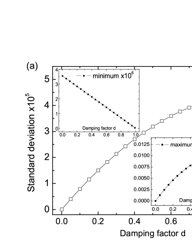
Figure 2: (Color online) (a) Standard deviation of the PR of the Stanford network, along with its minimum and maximum. The standard deviation of the PR gradually increases as the damping factor increases. In the insets: the minimum of the PR follows a trivial linear relation, while the maximum is nontrivially correlated with the value of the damping factor. (b) PR values of the three nodes having the highest PR are traced as the value of the damping factor is changed. Rank reversals occur around $d=0.55$ and $d=0.75$.

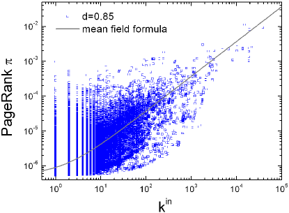
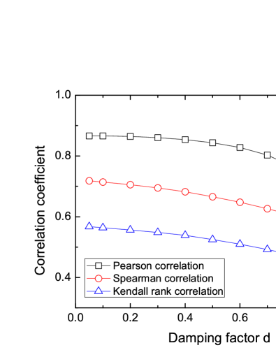
Figure 3: (Color online) The relationship between incoming degree and PR. The left panel clearly shows a positive correlation between the incoming degree and PR for $d_{0}=0.85$. It agrees well with the mean field result of Ref. [27], indicated by the solid line. The right-side panel shows the three different correlation coefficients between incoming degree and PR at different values of $d$. The correlation increases as the damping factor decreases.

We first examine the responses of PR to changes in the value of the damping factor $d$, as quantified by its standard deviation, minimum, and maximum. As can be seen from Fig. 2(a), the standard deviation of the PR gradually increases as the damping factor changes from zero to one. When the damping factor is zero, every PR is $1/N$ since in this regime only teleportation occurs. Therefore, both the minimum and maximum of the PR are $1/N$. The minimum of the PR (in Fig. 2(a), the left inset) decreases linearly as the damping factor increases since nodes with no incoming degree attain the minimum PR, $(1-d)/N$. However, the maximum of the PR is not trivial (in Fig. 2(a), the right inset). It seems to depend on the topology of the network. To understand the behavior of the maximum PR we follow the behavior of the three nodes of highest PR, as shown in Fig. 2(b). For any value of $d$, the maximum of PR is always associated to one of these nodes. These three nodes, situated in the giant SCC, show rank-reversal as the damping factor changes, thus accounting for the anomalous behavior of the maximum.

A correlation between incoming degree and PR has been reported by Fortunato et al. [27] and is confirmed in Fig. 3. The correlation coefficients between incoming degree and PR are $(r,r_{S},\tau)=(0.730,0.589,0.460)$ at $d=0.85$. As shown in the left-side panel, nodes with large incoming degree exhibit relatively narrow fluctuations in PR, while nodes of small degree show larger fluctuations. As the damping factor increases, the fluctuations of small degree nodes become broader and seem to induce smaller correlation coefficients at higher damping factors (See Fig. 3, the right-side panel). The correlation between PR and incoming degree, on the other hand, becomes higher as the random teleporting process increases. In that case, random walkers follow fewer steps in the network before teleporting and therefore sense only incoming degree, rather than higher-order link-link correlations.

6 Rank-reversal under damping factor perturbations

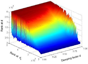
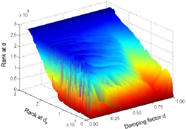
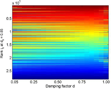
Figure 4: (Color online) Rank changes depending on the damping factor $d$. At $d_{0}=0.85$, nodes are sorted in descending order and are assigned an index $i_{0}$. Bottom figure: Color corresponds to the rank at the value $d$ given on the horizontal axis. Red represents the highest ranking and blue lowest. When the damping factor changes from 0.05 to 0.99, we observe how the rank changes. The top two plots give the rank changes in 3D (rank for $d$ is the z-axis). The rightmost plot is simply the leftmost plot shown from behind.

Figure 4 shows the overall change of the ranks for 281,903 nodes in response to damping factor changes away from $d_{0}=0.85$. We sort the nodes in descending order of PR at $d_{0}=0.85$ and assign to each node both a label $i_{0}$ as well as a corresponding color. Red represents the highest rank, blue the lowest. When the damping factor changes, we observe how the rank of each node changes. The top two plots give the rank changes in 3D (rank is the z-axis). The rightmost plot is the same as the leftmost plot but shown from behind. It demonstrates that rank changes occur often near the extremes of $d=0.05$ and $d=0.99$. Rank reverses near $d=0.85$ are quite apparent, and clear rank changes in this regime are observed over all nodes of the network. It seems that the middle-rank nodes show more rank change than do the top- and bottom-rank nodes near $d_{0}=0.85$.

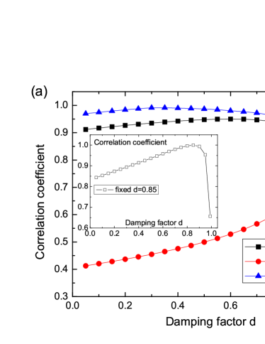
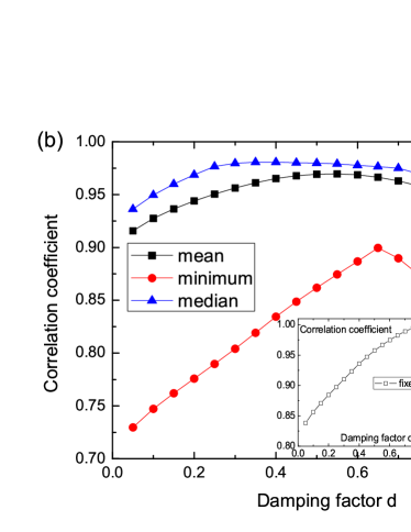
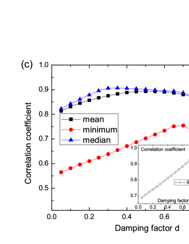
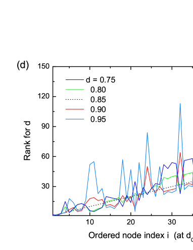
Figure 5: (Color online) The minimum, mean, and median of correlation coefficients of Pearson correlation (a), Spearman correlation (b), and Kendall rank correlation (c) between the PRs for different values of the damping factor. The inset of each figure illustrates the correlation coefficient between responses of PR at $d=0.85$ and its responses at the other damping factor values. (d) The 50 top-ranked nodes at $d=0.85$. While the damping factor changes by only 0.1 from 0.85, even the top 50 nodes are subject to relative rank fluctuations of up to three times their original rank.

In order to understand the sensitivity of PR to deviations in the value of the damping factor, we measure the correlation coefficients between two PR vectors at different $d$ values. For 20 values of the damping factor, $d=0.05,0.1,\cdots,0.95$ which are equally spaced except for the last one $d=0.99$, we compute the PRs and calculate correlation coefficients $C_{dd^{\prime}}$ of PR vectors for the 190 distinct damping factor pairs $(d,d^{\prime})$. For every $d$, we look at the minimum correlation coefficient $C_{d,\rm{min}}=\min_{d^{\prime}}C_{dd^{\prime}}$ at a given $d$, along with the mean and median of the distribution for the three correlation definitions. For comparison, we also compute these correlations for $d_{0}=0.85$ (the value used by Google), and display $C_{dd_{0}}$ in the inset of each plot for different correlation measures.

Figures 5(a)-(c) show the behaviors of the mean, median, and minimum of the three correlation coefficients for PR at a given damping factor $d$ compared to the other 19 values of the damping factor. The Pearson correlation in panel (a) shows that a peak of the minimum correlation coefficient line occurs around $d=0.90$ and decreases substantially for larger $d$. On the other hand, the other correlation coefficients, which are measurements of relative rank, place the peak of the minimum around 0.65. The relative rank given by PR is more stable around $d=0.65$ than it is around $d_{0}=0.85$ in this Stanford Web network, when we consider minimal rank-reversal. We do not know to what extent this result generalizes to other networks.

The panel insets relay the correlation coefficients between the PRs at $d_{0}=0.85$ and the other values of $d$. Observing these quantities, we can determine how much the PR changes when the damping factor increases or decreases by 0.05 around $d_{0}=0.85$. The Pearson correlation, in particular, suggests that the PR value is very sensitive to changes in $d$ when the damping factor is large. Rank changes in response to damping factor changes by 0.1 upward and downward are given in Fig. 5(d) for the 50 top-ranked pages at $d_{0}=0.85$. Remarkably, even the top-ranked nodes are subject to significant changes in rank (relative rank may change by up to three times its original value) when $d=0.95$. When $d$ increases 0.1 from $d_{0}=0.85$, the Kendall rank correlation becomes 0.918, which means roughly $1.6\times 10^{9}$ pairs (about 4% of the total pairs) are rank-reversed.

7 Rank-reversal in a single SCC

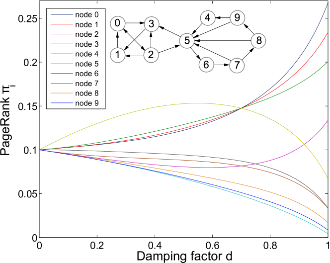
Figure 6: (Color online) Single SCC example of rank reversal. A directed network comprised of 10 strongly-connected nodes is, itself, a SCC without any dangling nodes or sinks. As can be seen in the figure, even this network undergoes rank reversal for high values of the damping factor.

As Boldi et al. discuss in their studies [15, 16], rank-reversals occur frequently in directed networks as a result of dangling nodes and rank-sinks. When the directed network contains a rank-sink, as the damping factor approaches 1 PR becomes trivially concentrated in the sink component(s). For this reason, choosing $d$ close to 1 does not give the best value of PR since many important nodes have a null PR in the limit $d\rightarrow 1$. In fact a similar effect occurs even when the directed network has no rank-sink, such as is the case with a single SCC.

To further explore this phenomenon, we examine a simple example of a directed network, comprised of 10 strongly-connected nodes (See Fig. 6). For this network, one can explicitly write down the 10 PR equations of Eq. (2):

$$\pi_{0}=d\left(\pi_{1}+\frac{\pi_{2}}{4}\right)+\frac{1-d}{10},\quad \pi_{1}=d\left(\pi_{3}+\frac{\pi_{2}}{4}\right)+\frac{1-d}{10},$$

$$\pi_{2}=d~{}\frac{\pi_{0}}{2}+\frac{1-d}{10}, \pi_{3}=d\left(\frac{\pi_{0}}{2}+\frac{\pi_{2}}{4}+\frac{\pi_{5}}{2}\right)+\frac{1-d}{10},$$

$$\pi_{4}=d~{}\frac{\pi_{9}}{2}+\frac{1-d}{10}, \pi_{5}=d\left(\pi_{4}+\frac{\pi_{2}}{4}+\frac{\pi_{7}}{2}+\frac{\pi_{8}}{2}+\frac{\pi_{9}}{2}\right)+\frac{1-d}{10},$$

$$\pi_{6}=d~{}\frac{\pi_{5}}{2}+\frac{1-d}{10}, \pi_{7}=d~{}\pi_{6}+\frac{1-d}{10},$$

$$\pi_{8}=d~{}\frac{\pi_{7}}{2}+\frac{1-d}{10}, \pi_{9}=d~{}\frac{\pi_{8}}{2}+\frac{1-d}{10}.$$

This system of 10 linear equations is solved and the results are plotted in Fig. 6 as a function of the damping factor $d$. While the network has only one SCC, rank reversals occur as the value of $d$ changes.

As one can see from this simple example, certain substructures of a network, like ‘pockets’ (rank-pockets), – in this example $\{0,1,2,3\}$ and $\{4,5,6,7,8,9\}$ – can concentrate the random walker inside causing rank-reversal. These structures could be modular structures like communities [8, 9]. In the above example, node 2 has outgoing degree 4. Among these outgoing links, however, only one link points toward the outside of the module, making a narrow channel. If we consider the extreme case that a node has very large outgoing degree $k^{\rm out}$ and all but one of the outgoing links of the node point toward the inside of the module (or rank-pocket) and only one link points outside, the pocket becomes a rank-sink in the limit $k^{\rm out}\rightarrow\infty$. In other words, the pocket becomes a trapping structure that is characterized by a vanishing ‘bottleneck’.

Uneven link density between modules (or other substructures) of a network allows pockets to concentrate random walkers inside, subsequently causing rank-reversal. These reversals call into question again: which damping factor $d$ is the best choice? In the example of Fig. 6, other centrality measures such as degree and betweenness centralities support node 5 as being the most important, but PR only supports this ranking when $d$ is less than about 0.7. The example, while simple, indicates that the best choice for damping factor may depend on the network structure, or on what features associated with a node’s position in a network one considers most important.

The structure of rank-pockets is very similar with that of ‘spam farms’ [28, 29]. These are groups of web pages that are intentionally interconnected to boost the PR of target pages giving them higher rankings than they deserve by “misleading” the PR’s link based algorithm. Since spam farms are continuously optimized through trial and error for Google’s ‘real’ damping factor and actual algorithm, filtering them is a challenging and outstanding computer science problem [29, 30].

8 Summary and concluding remark

Given that the success of modern businesses or the ranking of athletes [31], scientists [32], their papers [33], or scientific journals [8, 34] in which those papers are published depends on Google’s PageRank algorithm and its resulting ratings, it is far from a purely academic venture to understand rank-stability [35] and its dependence on network structure [36] and damping factor. Hence we have investigated PageRank (PR) as a function of its damping factor on a subset of pages from a single domain in the World Wide Web and found that rank-reversal occurs frequently and over a broader range of PR. We note that the Pearson correlation of PR between two different damping factors rapidly drops as the damping factor increases from the frequently-used value, 0.85. Rank-reversal is also observed by measuring the Spearman correlation and Kendall rank correlation. For this network the most stable value of the damping factor, in terms of relative rank, is about 0.65. This rank-reversal happens not only in directed networks containing rank-sinks but also in a single strongly connected component (SCC). This is due to the presence of rank-pockets and bottlenecks. When the damping factor approaches 1, PR converges trivially such that many important nodes have tiny PR possibly even within a single SCC. A better understanding rank-reversals may be essential to optimizing the stability of PR, to thwarting attempts to cheat such as spam farms, and ultimately to determining which scientists will be cited, which products will sell, and which businesses or other ventures will prosper.

Appendix A Stanford Web network

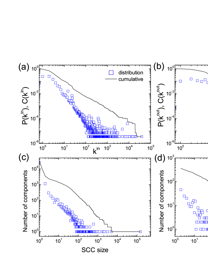
Figure 7: (Color online) (a) Incoming- and (b) outgoing-degree distributions and (c) SCC and (d) WCC size distributions for the Stanford Web network. The solid black line in each plot is the complementary cumulative distribution of the scatter plot.

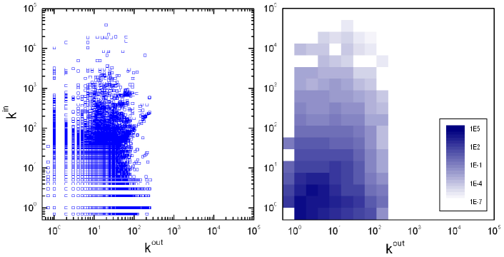
Figure 8: (Color online) Scatter plot of incoming and outgoing degrees for each node (left) and it density plot (right).

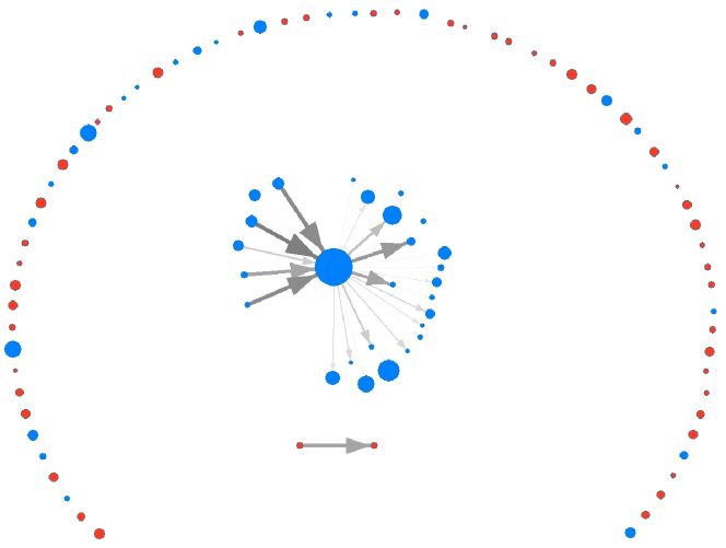
Figure 9: (Color online) SCC diagram for the Stanford Web network. For visualization, only the 98 largest SCCs have been displayed. Each circle corresponds to a SCC whose size is proportional to the logarithm of the number of nodes in the SCC. The SCCs in the largest WCC are colored blue, and the others red. The width and gray-scaled color of the directed links reflect their weight. Self-links are omitted. This SCC diagram shows a simple bow-tie structure.

The Stanford Web network we study exhibits a broad incoming degree distribution, that can be roughly characterized as a power-law $P(k)\sim k^{\gamma}$ with $\gamma\approx 2$, but its outgoing degree distribution is not easily classified (See Fig. 7(a), (b)). Looking at the degree-degree auto-correlation, the scatter plot of Fig. 8 shows no clear pattern in scatter plot. Only the density plot indicates a vague positive relationship between incoming and outgoing degrees in this network. The Pearson, Spearman, and Kendall correlations between incoming and outgoing degrees are 0.047, 0.258, and 0.206, respectively.

The Stanford Web data can be decomposed into 29,914 SCCs. Among these, 26,396 components have size 1, meaning that they are single nodes; the other 3,518 components consist of two or more nodes. The largest SCC contains 150,532 nodes– 53.4% of the total number of nodes in the network. We note that the Stanford data does not comprise a single connected network. Instead it contains 365 WCCs, the biggest of which consists of 255,265 nodes, or 90.6% of the total nodes in the network. The size distributions of the SCCs and the WCCs are displayed in the Fig. 7(c) and (d).

Figure 9 portrays the SCC structure of the 98 biggest SCCs in the Stanford Web data. For better visualization, only the 98 largest SCCs and their connecting links have been depicted. The smallest (98th) SCC in this diagram contains 162 nodes, and altogether, these 98 SCCs contain 198,123 nodes, which corresponds to 70.3% of the total nodes in the network. The size of each circle in Fig. 9 maps to the size of the corresponding SCC, and the color indicates whether a SCC lies inside or outside the giant WCC (blue is inside, and red is outside). As can be seen in Fig. 9, the network clearly exhibits a simple bow-tie structure [26].

References

References

- [1] Newman M E J 2003 SIAM Rev. 45 167
- [2] Colizza V, Barrat A, Barthelemy M and Vespignani A 2006 Proc. Natl. Acad. Sci. USA 103 2015
- [3] Wang P, González M C, Hidalgo C A and Barabási A-L 2009 Science 324 1071
- [4] Sood V and Redner S 2005 Phys. Rev. Lett. 94 178701
- [5] Baxter G J, Blythe R A and McKane A J 2008 Phys. Rev. Lett. 101 258701
- [6] Son S-W, Kim B J, Hong H and Jeong H 2009 Phys. Rev. Lett. 103 228702
- [7] Kim D-H and Motter A E 2009 New J. Phys. 11 113047
- [8] Rosvall M, Bergstrom C T 2008 Proc. Natl. Acad. Sci. USA 105 1118
- [9] Kim Y, Son S-W and Jeong H 2010 Phys. Rev. E 81 016103
- [10] Masuda N, Kawamura Y and Kori H 2009 New Journal of Physics 11 113002
- [11] Brin S and Page L 1998 Comput. Netw. ISDN Syst. 30 107
- [12] Borodin A, Roberts G O, Rosenthal J S and Tsaparas P 2001 In Proceedings of the 10th International World Wide Web Conference, Hong Kong 415
- [13] Hughes R D 1995 Random Walks and Random Environments, Vol. 1: Random walks (Clarendon, Oxford)
- [14] Noh J D and Rieger H 2004 Phys. Rev. Lett. 92 118701
- [15] Boldi P, Santini M and Vigna S 2005 Proceeding WWW ’05 Proceedings of the 14th international conference on World Wide Web 557
- [16] Boldi P, Santini M and Vigna S 2009 ACM Transactions on Information Systems 27 19
- [17] Pretto L 2002 LNCS 2476 131
- [18] Langville A N and Meyer C D 2003 Internet Mathematics 1 335
- [19] Lempel R and Moran S 2005 Information Retrieval 8 245
- [20] Tarjan R 1972 SIAM J. Comput. 1 146
- [21] Wilcox R 2005 Introduction to Robust Estimation and Hypothesis Testing, 2nd edition, Academic Press
- [22] Raschke M, Schläpfer M and Nibali R 2010 Phys. Rev. E 82 037102
- [23] http://snap.stanford.edu/data/web-Stanford.html
- [24] Leskovec J, Lang K, Dasgupta A and Mahoney M 2009 Internet Mathematics 6 29
- [25] Son S-W, Christensen C, Bizhani G, Foster D V, Grassberger P and Paczuski M 2012 e-print arXiv:1201.1507
- [26] Broder A et al. 2000 Computer Networks 33 309
- [27] Fortunato S, Boguñá M, Flammini A and Menczer F 2007 Internet Mathematics 4 245
- [28] Gyöngyi Z and Garcia-Molina H 2005 Proceedings of the First International Workshop on Adversarial Information Retrieval on the Web, Chiba, Japan
- [29] Du Y, Shi Y and Zhao X 2007 Proceedings of the 3rd International Workshop on Adversarial Information Retrieval on the Web, Banff, Alberta, Canada
- [30] Han S, Ahn Y-Y, Moon S and Jeong H 2006 Proceedings of International World Wide Web Conference, Workshop on the Weblogging Ecosystem
- [31] Radicchi F 2011 PLoS ONE 6 e17249
- [32] Radicchi F, Fortunato S, Markines B and Vespignani A 2009 Phys. Rev. E 80 056103
- [33] Chen P, Xie H, Maslov S and Redner S 2007 Journal of Infometrics 1 8
- [34] Bergstrom C T and West J 2008 Neurology 71 1850
- [35] Ng A Y, Zheng A X and Jordan M I 2001 Proceedings of the 24th International Conference on Research and Development in Information Retrieval (SIGIR) 258
- [36] Ghoshal G and Barabasi A-L 2011 Nature Communications 2 394