A Realistic Treatment of Geomagnetic Cherenkov Radiation
from Cosmic Ray Air Showers

Abstract

We present a macroscopic calculation of coherent electro-magnetic radiation from air showers initiated by ultra-high energy cosmic rays, based on currents obtained from three-dimensional Monte Carlo simulations of air showers in a realistic geo-magnetic field. We discuss the importance of a correct treatment of the index of refraction in air, given by the law of Gladstone and Dale, which affects the pulses enormously for certain configurations, compared to a simplified treatment using a constant index. We predict in particular a geomagnetic Cherenkov radiation, which provides strong signals at high frequencies (GHz), for certain geometries together with “normal radiation” from the shower maximum, leading to a double peak structure in the frequency spectrum. We also provide some information about the numerical procedures referred to as EVA 1.0.

I Introduction

The aim of our work is to provide a realistic calculation of radio emission from air showers, which might be used finally to analyze and understand the results from radio detection experiments (LOPES Fal05 ; Ape06 , CODALEMA Ard06 , LOFAR lofar2 ), and the new set-ups at the Pierre Auger Observatory (MAXIMA auger1 , AERA auger2 ).

There are two ways to compute the electric fields created by the moving charges of air showers: the “macroscopic approach” adds up the elementary charges and currents to obtain a macroscopic description of the total electric current in space and time, which is the source of the electric field obtained from solving Mawell’s equations. The “microscopic approach” computes the fields for each elementary charge, and adds then all the fields (with a large amount of cancellations).

Already in the earliest works of  Jel65 ; Por65 ; Kah66 ; All71 , a macroscopic treatment of the radio emission was proposed, but at the time the assumptions about the currents were rather crude. There is recent progress concerning the macroscopic approach. In 2007, we performed calculations allowing under simplifying conditions to obtain a simple analytic expression for the pulse shape, showing a clear relation between the pulse shape and the shower profile olaf . This allows, for example, to determine from the radio signal the chemical composition krijn2 of the cosmic ray. The picture used was very similar to the one in Ref. Kah66 , which has been refined by using a more realistic shower profile and where we calculate the time-dependence of the pulse. Recently it was confirmed that the pulse predicted in the microscopic description huegear1 ; alvarez agrees with the predictions following from the macroscopic picture as shown in huegear2 .

In Ref. klaus1 , we advance further by computing first the four-current from a realistic Monte Carlo simulation (in the presence of a geo-magnetic field), and then solve the Maxwell equations to obtain the electric field, while considering a realistic (variable) index of refraction, given by the Gladstone-Dale law as

$$n=n_{GD}=1+0.226\frac{\mathrm{cm^{3}}}{g}\rho(h),$$ (1)

with $\rho(h)$ being the density of air at an atmospheric height $h$. Although this index varies only between 1 and 1.0003, this variation has important consequences, as discussed in detail in Ref. klaus1 . For example, the retarded time $t^{*}$ (the time when the signal was sent out) for a given observer position is a multivalued function of the observer time $t$, which gives rise to “Cherenkov effect” phenomena, where the signal may become very short and very strong. The caveat in this treatment is the fact that we consider the currents to be point-like, which is only a good approximation far from the shower axis. The Cherenkov-like effects actually show up as singularities, and we expect these singularities to disappear when we give up the “point-like” assumption. Nevertheless, although Ref. klaus1 does not provide a realistic picture for all observer distances, its results are very important as the basis of the much more realistic description employed in the present paper.

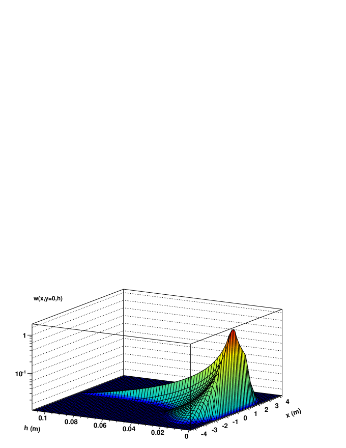
Figure 1: The distribution of charged particles $w(x,y,h)$ at a given time, as a function of the transverse coordinate $x$ and the longitudinal coordinate $h$, for $y=0$.

Anyhow, the notion “point-like” has to be taken with care. In the point-like picture described in Ref. klaus1 , we do not have a simple moving point-like charge, we rather have already transverse currents, and also the longitudinal structure is nontrivial, just all these currents are – at a given time – concentrated in a very small volume. But there must be an internal structure, and therefore it is natural as a next step to investigate the three-dimensional structure of the shower at a given time. In order to do so, we consider a “shower fixed” coordinate system. The origin $O$ of this system is the center of the shower front. We use the coordinates $x$ and $y$ to describe positions in the plane transverse to the shower axis, and $h$ as the longitudinal distance behind the shower front. The latter one is actually a hypothetical plane, which contains real particles only around $x=y=0$, whereas for larger distances, the fastest particles stay behind this plane. The situation as obtained in a realistic Monte Carlo simulation (details to be discussed later) is shown in fig. 1. The distribution of charged particles shows a very sharp maximum at the origin ($x=y=h=0)$, and falls steeply in transverse and longitudinal direction. We will discuss the functional form of this distribution later in detail, for the moment we only want to illustrate the fact that the distribution obtained from simulations shows nontrivial structures, concentrated in a small range in particular concerning the $h$ variable.

In the current paper, we want to take into account the realistic three-dimensional form (at a given time) of the shower, as obtained from shower simulations, still using a realistic index of refraction. The numerical procedures of our approach, referred to as EVA 1 (Electric fields, using a Variable index of refraction in Air shower simulations), amount to air shower simulations, analysis tools for extracting currents and shower shapes, and automatic fitting procedures providing smooth functions for all relevant shower characteristics. First results of our new approach have been published recently krijn . In the last part of the paper, we discuss important consequences of our approach, referred to as “geomagnetic Cherenkov radiation”, which provides strong emissions in the GHz frequency domain, alone or as double peak structures in the frequency spectrum.

II Taming singularities

We first repeat some elementary facts of the shower evolution, which have been discussed in detail in Ref. klaus1 . We consider here showers due to a very energetic primary particle, with an energy above $10^{14}\,\mathrm{eV}$. Such a shower moves with a velocity $\beta c$, which is very close to the vacuum velocity of light $c$. There is a constant creation of electrons and positrons at the shower front, with somewhat more electrons than positrons (electron excess). This is compensated by positive ions in the air, essentially at rest. The electrons and positrons of the shower scatter and lose energy, and therefore they move slower than the shower front, falling behind, and finally drop out as “slow electrons / positrons”. Close to the shower maximum, the charge excess of the “dropping out” particles is compensated by the positive ions, since there is no current before or behind the shower. Taking all together we have the situation of a moving charge, moving with the vacuum velocity of light, even though the electrons and positrons are moving slower, and they are deviated (in opposite directions) in the Earth magnetic field.

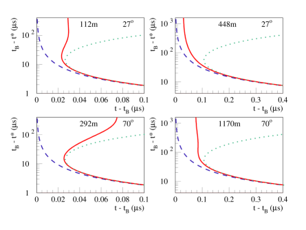
Figure 2: The dependence of the retarded time $t^{*}$ on the observer time $t$ for $n=1$ (dashed line), $n=n_{GD}$ (solid line), and $n=n_{\mathrm{ground}}\approx 1.0003$ (dotted line) for inclined showers (27^o and 70^o and for different distances in meters of the observer from the impact). The reference time $t_{B}$ is the time of closest approach of the shower with respect to the observer.

Neglecting the finite dimension of the shower, referred to as “point-like” (PL) approximation, one has a four-current

$$j_{\mathrm{PL}}(t^{\prime},\vec{x})=J(t^{\prime})\,\delta^{3}(\vec{x}-\vec{\xi}(t^{\prime})),$$ (2)

with a longitudinal component due to charge excess, and a transverse component due to the geo-magnetic field. Solving Maxwell’s equations, we can express the potential in terms of the four-current $J$, evaluated at the retarded time $t^{*}$, as klaus1

$$A_{\mathrm{PL}}^{\beta}(t,\vec{x})=\frac{\mu_{0}}{4\pi}\,\frac{J^{\beta}}{|\widetilde{R}V|}\,,$$ (3)

with $V=c^{-1}d\xi/dt^{\prime}$, and with $\widetilde{R}$ being a four-vector defined as $\widetilde{R}{}^{0}=c(t-t^{*})$ and $\widetilde{R}{}^{i}=-L\partial/\partial\xi^{i}L,$ where $L$ is the optical path length between the source $\vec{\xi}(t^{*})$ and the observer. This point-like approximation is certainly only valid at large impact parameters ($>500\,\mathrm{m}$), but even more importantly it will serve as a basis for more realistic calculations, as discussed later. It should be noted that in case of $n>1$ and even more for $n=n_{GD}$ the vector potential shows singularities, which arise from $1/|\widetilde{R}V|\propto$ $dt^{*}/dt$ and the fact that $t^{*}$ is a non-monotonic function of $t$, as shown in fig. 2 and discussed in detail in klaus1 . We show the realistic case $n=n_{GD}$ with the corresponding curve situated between the two limiting cases $n=1$ and $n=1.0003$.

In general, one needs to consider the finite extension of the shower at a given time $t^{\prime}$, expressed via a weight function $w(r^{1},r^{2},h)$, where $r^{1}$ and $r^{2}$ represent the transverse distance from the shower axis, and $h$ the longitudinal distance from the shower front, the latter one moving by definition with the vacuum velocity of light. Positive $h$ means a position behind the shower front, and therefore $w$ is non-vanishing only for positive $h$. The weight will fall off rapidly with increasing distance $r=\sqrt{(r^{1})^{2}+(r^{2})^{2}}$ from the axis. The precise form of $w$ will be discussed in a later chapter. In principle one needs to convolute the weight $w$ with the currents, and then compute the potential and field. Due to a translation invariance (being correct to a very good approximation, since the index of refraction varies slowly), this is the same as computing first the potential in PL approximation, and then performing a convolution as

$$A^{\beta}(t,\vec{x})=\int\!\!d^{2}r\!\!\int\!\!dh\,w(\vec{r},h)A_{\mathrm{PL}}^{\beta}(t,x^{\|}-h,\vec{x}^{\perp}+\vec{r}).$$ (4)

where $x^{\|}$ and $\vec{x}^{\bot}=(x^{\bot 1},x^{\bot 2})$ are coordinates parallel and transverse to the shower axis. Defining $\vec{y}^{\bot}=\vec{x}^{\bot}+\vec{r}$, we get

$$A^{\beta}(t,\vec{x})=\int\!\!d^{2}y^{\bot}\!\!\int\!\!dh\,w(\vec{y}^{\bot}-\vec{x}_{\perp},h)A_{\mathrm{PL}}^{\beta}(t,x^{\|}-h,\vec{y}^{\bot}).$$ (5)

The electric field is then obtained from the derivatives of $A$.

One cannot simply exchange derivation and integration, due to the presence of singularities as discussed before, and therefore a naive convolution of $w$ with $\vec{E}_{\mathrm{PL}}$ is not possible: one needs a more sophisticated treatment of the singularities. So let us consider the most general case of a multi-valued function $t^{*}$ as a function of the observation time $t$, as sketched in fig. 3.

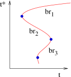
Figure 3: Several branches of the function of $t^{*}$ versus $t$, where $t^{*}$ is the retarded time corresponding to an observer time $t$ .

The function is composed of several branches, $\mathrm{br}_{n}$, limited by certain times $t_{k}$. The derivative $dt^{*}/dt$ becomes infinite at these branch endpoints, and the point-like potential becomes singular. This is why we refer to the $t_{k}$ as ”critical times”. Close to these singularities, we have

$$t^{*}-t^{*}(t_{k})\sim|t-t_{k}|^{1/2},\quad\mathrm{and}\quad\frac{dt^{*}}{dt}\sim|t-t_{k}|^{-1/2}.$$ (6)

When evaluating eq. (5), we have to worry about the critical time for a given observer position $(x^{\|}-h,\vec{y}^{\bot})$, corresponding to the arguments of $A_{\mathrm{PL}}$. In other words, $t_{k}$ is a function of these variables, i.e.

$$t_{k}=t_{k}(x^{\|}-h,\vec{y}^{\bot}).$$ (7)

It is useful to define a “critical $h$ value” $h_{k}$, for given $t$, via

$$t=t_{k}(x^{\|}-h_{k},\vec{y}^{\bot}),$$ (8)

which allows us to write eq. (5) for a single branch as

$$A^{\beta}(t,\vec{x}) =\int\!\!d^{2}y^{\bot}\!\!\int_{0}^{h_{k}}\!\!dh\,w(\vec{y}^{\bot}-\vec{x}^{\bot},h)$$

$$\qquad A_{\mathrm{PL}}^{\beta}(t,x^{\|}-h,\vec{y}^{\bot}).$$ (9)

Using the integration variable $\lambda=h_{k}-h$, we obtain our master formula for the vector potential,

$$A^{\beta}(t,\vec{x}) =\int\!\!d^{2}y^{\bot}\!\!\int_{0}^{h_{k}}\!\!d\lambda\,w(\vec{y}^{\bot}-\vec{x}^{\bot},h_{k}-\lambda)$$

$$\qquad A_{\mathrm{PL}}^{\beta}(t,x^{\|}-h_{k}+\lambda,\vec{y}^{\bot}),$$ (10)

which is useful because $A_{\mathrm{PL}}$ has a singularity in $\lambda\>$ for
$\lambda\to 0$, which does not interfere with the derivatives which have to be performed in order to get the fields. In the following we keep in mind that $A_{\mathrm{PL}}^{\beta}$ has the following arguments: the time $t$, the longitudinal variable $x^{\|}-h_{k}+\lambda$, and the transverse variable $\vec{y}_{\perp}$; $w$ has the arguments $h_{k}-\lambda$ and $\vec{y}_{\perp}-\vec{x}_{\perp}$. We do not write these arguments explicitly, to simplify the notation. We also omit the arguments $t,\vec{x}$ of the vector potential. So we write

$$A^{\beta}=\int\!\!d^{2}y^{\bot}\!\!\int_{0}^{h_{k}}\!\!d\lambda\,w\,A_{\mathrm{PL}}^{\beta}.$$ (11)

The components of the electric field are

$$E^{\|}=c(-\frac{\partial A^{0}}{\partial x^{\|}}-\frac{\partial A^{\|}}{\partial\,ct})$$ (12)

$$E^{\bot i}=c(-\frac{\partial A^{0}}{\partial x^{\bot i}}-\frac{\partial A^{\bot i}}{\partial\,ct}).$$ (13)

Using $A_{\mathrm{PL}}^{i}=\frac{\mu_{0}}{4\pi}\,J^{i}\,|\widetilde{R}V|^{-1}$ and eqs. (31,32), the time derivative of the vector potential may be written as

$$\frac{\partial A^{i}}{\partial\,ct}=\int d^{2}y_{\perp}\!\!\int_{0}^{h_{k}}\!\!d\lambda\,\left\{-w^{\prime}\,A_{\mathrm{PL}}^{i}+w\,\dot{A}_{\mathrm{PL}}^{i}\right\},$$ (14)

with $w^{\prime}=\partial w/\partial h$, $\dot{A}_{\mathrm{PL}}^{i}=\frac{\mu_{0}}{4\pi}\,K^{i}\,|\widetilde{R}V|^{-1}$, $K=dJ/dt^{\prime}$. In principle there is an additional term from the time derivative of the upper limit of integration, but this contribution vanishes due to $w(0)=0$ (see next chapter). Concerning the space derivative, we first compute the derivative with respect to the longitudinal variable. We find

$$-\frac{\partial}{\partial x^{\|}}A^{0}=-\int d^{2}y_{\perp}\!\!\int_{0}^{h_{k}}\!w^{\prime}\,A_{\mathrm{PL}}^{0}\!d\lambda\,$$ (15)

since the total longitudinal space derivative of $A_{\mathrm{PL}}^{0}$ vanishes exactly. The transverse derivatives of the scalar potential can be expressed in terms of the derivatives $w^{i}=\partial w/\partial r^{i}$ of the weight function $w$ as

$$-\frac{\partial}{\partial x^{\bot i}}A^{0}\!=\!\int\!d^{2}y_{\perp}\!\int_{0}^{h_{k}}\!\!d\lambda\,w^{i}\,A_{\mathrm{PL}}^{0}.$$ (16)

The above results for the partial derivatives of the vector potential $A^{\mu}$ allow us to obtain corresponding expressions for the electric field. The longitudinal electric field $c(\partial^{\|}A^{0}-\partial^{0}A^{\|})$ is given as

$$E^{\|}=-c\!\int\!d^{2}y_{\perp}\!\int_{0}^{h_{k}}\!\!d\lambda\,\left\{w^{\prime}\,A_{\mathrm{PL}}^{0}-w^{\prime}\,A_{\mathrm{PL}}^{\|}+w\,\dot{A}_{\mathrm{PL}}^{\|}\right\}.$$ (17)

The transverse field $c(\partial^{\bot i}A^{0}-\partial^{0}A^{\bot i})$ can be written as

$$E^{\bot i}=c\int\!\!d^{2}y_{\perp}\!\!\int_{0}^{h_{k}}\!\!d\lambda\left\{w^{i}\,A_{\mathrm{PL}}^{0}+w^{\prime}\,A_{\mathrm{PL}}^{\bot}-w\,\dot{A}_{\mathrm{PL}}^{\bot}\right\}.$$ (18)

The formulas simplify considerably far from the singularity as well as at the singularity, but we keep the exact expressions, in order to interpolate correctly between the two extremes. It should be noted that the above expression concerns a single branch, the complete field is the sum over all branches.

In the present work we have derived the electric field directly from the Li nard-Wiechert potentials in the Lorentz gauge without further approximations. The distribution of the particles in the shower front over a finite volume is the reason that our final result is not plagued with singularities in the vicinity of Cherenkov emission. We thus explicitly include both the near- and the far-field components of the radiation. In this sense it differs considerably from the calculations presented in alvarez where an ad-hoc frequency cut-off is introduced in the calculations of $300$ MHz, and the near-field component of the electric field is neglected (the Fraunhofer condition). As can be seen from fig. 26 below, the data show a considerable intensity above $300$ MHz. A question that arises in this respect is the validity of the Fraunhofer condition when Cherenkov effects come into play which implicitly is assumed in alvarez . Often the Fraunhofer condition is formulated as $a^{2}\sin^{2}\theta/R<\lambda/2\pi\;,$where $a$ is the length of the emission trajectory, $\theta$ is the opening angle from the emission point to the observer, $\lambda$ the wavelength of the emitted signal, and $R$ the distance from the emission point to the observer. If there is a single point on $a$ where the Cherenkov condition is fulfilled, the electric field will diverge at this point whereas the field is finite at all other points. This implies that thus the Fraunhofer condition is not valid. A Lorentz-invariant formulation of the Fraunhofer condition is $a^{2}\sin^{2}\theta/\tilde{R}V<\lambda/2\pi,$ where the distance $R$ is replaced by the retarded distance $\tilde{R}V$. Since the retarded distance vanishes at the Cherenkov angle this clearly shows that at this point the Fraunhofer condition is no longer valid for which reason we have not made this assumption in our approach.

III Monte Carlo simulations and fitting procedures: EVA 1.0

The numerical evaluation of the eqs. (17,18) is done employing the EVA 1.0 package, which

• provides the weights $w$,

• provides the currents $J$ needed to compute the potentials $A_{\mathrm{PL}}^{\mu}$,

• does the numerical integration of eqs. (17,18) and the summation over branches.

Both the weights $w$ and the point-like currents $J$ are obtained from realistic Monte Carlo simulations of air showers. The EVA package consists of several elements:

• the air shower simulation code CX-MC-GEO, including analysis tools to extract four-currents and the shape of the shower,

• the automatic fitting procedure FITMC which allows to obtain analytical expressions for the currents,

• the EVA program which solves the non-trivial problem to compute the retarded time and “the denominator” $\tilde{R}V$, for a realistic index of refraction.

We first discuss air showers. They are considered point-like for the moment, as seen by a far-away observer. The shower is a moving point, defining a straight line trajectory, see fig. 4 .

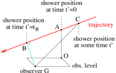
Figure 4: Air shower as seen by an observer $G$. The point $B$ is the point of closest approach with respect to the observer $G$. The point $C$ is the shower position at some time $t^{\prime}$. The point $B$ corresponds to the shower position at $t^{\prime}=t_{B}$ (which may be taken to be zero).

One defines an “observer level” which is a plane of given altitude $z$ with respect to the sea level. One defines some arbitrary point $A$ on the trajectory. The corresponding projection to the observer level is named $O$ (origin) and the observer position is given in terms of coordinates $(x,y)$ with respect to $O$. The $x-$axis is the intersection of the “shower plane” $OAC$ and the observer level. The angle between the shower trajectory and the vertical axis $OA$ is referred to as inclination and denoted as $\theta$. In many applications, $A$ and $O$ coincide: in this case they represent the impact point. For horizontal showers the two points are different. The geomagnetic field is specified by an angle $\alpha$ with respect to the vertical, and an angle $\psi$ with respect to the shower plane ($\psi=0$ means that $\vec{B}$ points towards the shower origin). One can of course see it the other way round (maybe even more natural): for a given orientation of the geomagnetic field, $\psi$ defines the orientation of the shower axis.

In the EVA framework, one has to specify the altitude $z$, the distance $a=|OA|$, the inclination $\theta$, the energy $E$ of the shower, and the observer coordinates $x$, $y$. And in addition the angles $\alpha$ and $\psi$ and the magnitude $B$ of the geomagnetic field.

The actual air shower simulations are done with a simulation program called CX-MC-GEO, being part of the EVA package. It is based on CONEX conex1 ; conex2 , which has been developed to do air shower calculations based on a hybrid technique, which combines Monte Carlo simulations and numerical solutions of cascade equations. It is also possible to run CONEX in a pure cascade mode, and this is precisely what we use. This provides full Monte Carlo air shower simulations, using EGS4 egs4 for the electromagnetic cascade, and the usual hadronic interaction models (QGSJET, EPOS, etc) to simulate hadronic interactions.

Two features have been added to CONEX. First of all a magnetic field, which amounts to replacing the straight line trajectories of charged particles by curved ones. This concerns both the electromagnetic cascade and the hadronic one. In addition, analysis tools have been developed, which allow to get a complete information of charged particle flow in space and time. These features have already been developed to compute currents in klaus1 , so in particular more details about the implementation of the magnetic field can be found there (though we did not use the names EVA and CX-MC-GEO yet). We also discuss in klaus1 some details about the different internal coordinate systems needed to extract information about currents. The results shown in krijn were also based on CX-MC-GEO simulations, referred to as CONEX-MC-GEO at the time.

In klaus1 , we provide several results concerning particle numbers and currents for different orientations of the axis with respect to the geomagnetic field. All the results are still valid, the corresponding programs did not change since.

An important ingredient of our approach is the parametrization of the results (currents $J$, distributions $w$), which have been obtained from simulations in the form of discrete tables. This is necessary partly to perform semi-analytical calculations such that numerically stable functions have to be dealt with without having huge cancellations in the results. It is especially important for the stable calculation of Cherenkov effects. It allows for the calculation of a smooth shower evolution, whereas when working with histogramed distributions in position and time, it is not possible to reconstruct a continuous shower evolution and the artificially introduced sudden changes in the particle trajectories may give rise to spurious radio signals.

The parametrization of Monte Carlo distributions is done in FITMC. This program takes the distributions (for currents) as obtained from the simulations in the form of histograms, to obtain analytical expressions, using standard minimization procedures. FITMC creates actually computer code to represent the analytical functions, and this code is then executed at a later stage. The “basic distribution” is the so-called “electron number $N$” (which counts the number of electrons and positrons) as a function of the shower time $t^{\prime}$, which is fitted as

$$N(t^{\prime}) =A\,\exp\big{(}B+C(t^{\prime}+D)$$ (19)

$$\qquad\qquad\qquad+E(t^{\prime}+F)^{2}+G(t^{\prime}+H)^{3}\,\big{)}.$$

As an illustration, we show here the case of a shower with an initial energy of $5\cdot 10^{17}$eV, an inclination $\theta=27^{0}$, and an azimuth angle $\psi=0^{0}$, defined with respect to the magnetic north pole. The angle $\psi$ refers to the origin of the shower. So $\psi=0^{0}$ thus implies that the shower moves from north to south. We consider the magnetic field at the CODALEMA site, i.e. $|\vec{B}|=47.3\mu T$ and $\alpha=153^{0}$, so the shower makes an angle of roughly $54^{0}$ with the magnetic field.

In fig.5,

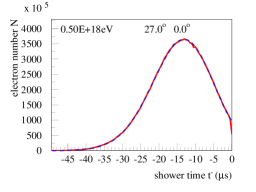
Figure 5: The number $N$ of electrons and positrons, as a function of the shower time $t^{\prime}$ for a shower with an inclination $\theta=27^{0}$ and an azimuth angle $\psi=0^{0}$ with respect to the magnetic north pole. The full red line represents the simulation result, the dashed blue line is the fit.

we plot the electron number $N$, as a function of the shower time $t^{\prime}$, for a simulated single event, together with the fit curve. A thinning procedure has been applied (here and in the following) to obtain the shown simulation results. The time $t^{\prime}=0$ refers to the point of closest approach with respect to an observer at $x=0$, $y=500\,$m, $z=140\,$m. We suppose $a=0$ (so the shower hits the ground at $x=y=0$).

The magnitudes of the components $J^{\mu}$ of the currents have a similar $t^{\prime}$ dependence as $N(t^{\prime})$. Therefore we parametrize the ratios $J^{\mu}/(Nec)$, with $N$ being the electron number, $e$ the elementary charge, and $c$ the velocity of light. We use the following parametric form:

$$\frac{J^{\mu}(t^{\prime})}{N(t^{\prime})ec}=A+B(x+C)+D(x+E)^{2}+F(x+G)^{3}.$$ (20)

In fig. 6,

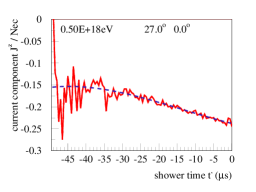
Figure 6: The longitudinal current component $J^{z}$, divided by $Nec$, as a function of the shower time $t^{\prime}$. The full red line represents the simulation result, the dashed blue line is the fit.

we plot the longitudinal current component $J^{z}$ (divided by $Nec)$, as a function of the shower time $t^{\prime}$, for a simulated single event, together with the fit curve. At early times - far away from the shower maximum – there are of course large statistical fluctuations. But since $N(t^{\prime})$ is very small here, this region does not contribute to the pulse. In fig. 7,

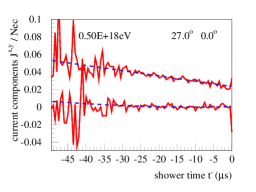
Figure 7: The transverse current components $J^{x}$ (lower lines) and $J^{y}$ (upper lines), divided by $Nec$, as a function of the shower time $t^{\prime}$. The full red lines represents the simulation result, the dashed blue lines are the fits.

we plot the transverse current components $J^{x}$ and $J^{y}$, (divided by $Nec)$, as a function of the shower time $t^{\prime}$, for a simulated single event, together with the fit curves.

The EVA program uses these analytical fit functions for the current components,

$$J^{\mu}=\left\{\frac{J^{\mu}}{Nec}\right\}_{fit}\cdot N_{fit}\cdot e\cdot c,$$ (21)

to compute the vector potential. The currents have to be evaluated at $t^{\prime}=t^{*}$, the retarded time. The central part of EVA is actually the determination of the retarded time $t^{*}(t,\vec{x}$) for a given observer position. This is quite involved – in case of a realistic index of refraction – and described in detail in klaus1 (again without referring to EVA, but these are exactly the same programs being used). A results of such a calculation is shown in fig. 21.

A new feature compared to klaus1 – and most relevant for this paper – is the possibility to obtain information about the shape of the shower via the weight function $w$. The weight function $w$ is not perfectly cylindrically symmetric, due to the geo-magnetic field but also due to statistical fluctuations, since we are considering individual Monte Carlo events. However, in this paper we will neglect these tiny deviation from symmetry, and consider a weight function $w(r,h)$ depending only on the two variables $r$ and $h$, related to the general weight function as

$$w(r,h)=2\pi r\,w(\vec{r},h).$$ (22)

The lateral coordinate $r$ measures the transverse distance from the shower axis, the longitudinal coordinate $h$ is meant to be the distance behind the shower front. This front is a hypothetical plane moving parallel to the shower axis with the velocity of light $c$, such that all the particles are behind this front, expressed by a positive value of $h$. We will express the weight function as

$$w(r,h)=w_{1}(r)\,w_{2}(r,h),$$ (23)

with $\int dr\,w_{1}(r)=1$, and with $\int dh\,w_{2}(r,h)=1$ for all values of $r$.

We use again CX-MC-GEO to obtain $w$, then FITMC to obtain an analytical function, which is later used in the EVA program to compute the fields, based on the formulas described in the preceding chapter. All the simulation results shown in the following are based on the the same shower, mentioned earlier when discussing currents.

We first investigate the radial distribution $w_{1}(r)$.

Figure 8: The radial distribution $w_{1}(r)$. The thin yellow lines correspond to different times, the points represent an average, and the thick red line corresponds to a fit (see text).

In fig. 8, we show the radial distribution as obtained from the Monte Carlo simulation. The thin lines correspond to different times $t^{\prime}$, between $-25\,\mu s$ and $-5\,\mu s$. The points represent an average over all times, and also averaged over $r$–bins. Since the time dependence is quite small, we will use the radial distribution at the shower maximum $t^{\prime}_{\max}$ as time-independent distribution $w_{1}(r)$. The thick red line corresponds to a fit to the Monte Carlo data, using the form

$$w_{1}(r)=\frac{\Gamma(4.5-s)}{\Gamma(s)\Gamma(4.5-2s)}\left(\frac{r}{r_{0}}\right)^{s-1}\left(\frac{r}{r_{0}}+1\right)^{s-4.5},$$ (24)

with fit parameters $r_{0}$ and $s$ (providing an excellent fit).

Knowing $w_{1}(r)$, we now investigate how far the particles are moving behind the shower front, expressed in terms of the longitudinal distance $h$, for a given transverse distance $r$. From the above simulation, we obtain easily the mean distance $\bar{h}$ at a given $r$. We find a perfectly linear time dependence, of the form

$$\bar{h}=h_{\mathrm{front}}+c\Delta\beta\,t^{\prime},$$ (25)

where $\Delta\beta$ can be obtained from fitting time dependence at different distances $r$, the result is shown in fig. 9 as solid line.

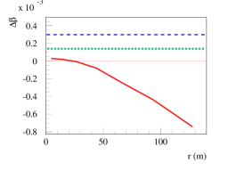
Figure 9: The longitudinal velocity difference $\Delta\beta$ versus $r$. We show the results for realistic simulations (thick red solid line) and for $\gamma=60$ (green dotted line). Also shown: the value $1-1/n_{\mathrm{ground}}$(blue dashed line).

The quantity $\Delta\beta$ represents the velocity difference (in units of $c$) with respect to the the shower front, which itself moves with velocity $c$. So the velocity of the “average position” of the shower is $1-\Delta\beta$. Also shown in fig. 9, as dashed line, is the value $1-1/n_{\mathrm{ground}}$, corresponding to the velocity of light in air with $n_{\mathrm{ground}}=1.0003$. And we also plot as dotted line the $\Delta\beta$ obtained from $\gamma=60$, corresponding to the average electron energy. The simulated curve (thick full line) is considerably below this dashed and the dotted curves, which means that the velocity of the average positions is larger than $c/n_{\mathrm{ground}}$, it is also larger than the velocity of the average electron. The simulated velocity is even (slightly) larger than $c$. This is due to the fact that matter is moving on the average from inside (small $r$) to outside (large $r$), and the average $\bar{h}$ decreases with decreasing distance $r$. But the effect is small, the deviation of the shower velocity from $c$ is less than 1/1000.

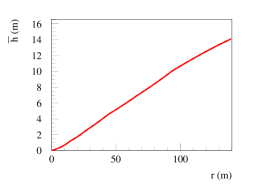
Figure 10: The mean value $\bar{h}$ for given values of the lateral distance $r$.

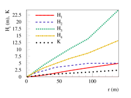
Figure 11: The parameters $H_{1}$, $H_{2}$, $H_{3}$, $H_{4}$, and $K$ as a function of the lateral distance: $H_{1}$ (full line) , $H_{2}$ (dashed line) , $H_{3}$ (dotted line), $H_{4}$ (dashed-dotted line) , $K$ (wide-dotted line) ,

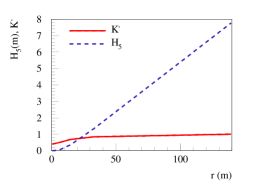
Figure 12: The parameters $H_{5}$ and $K^{\prime}$ as a function of the lateral distance: $K^{\prime}$ (full line) , $H_{5}$ (dashed line)

We will ignore the small time dependence for the moment, and consider in the following quantities at $t_{\max}$. To get some idea about the typical scales of the $h$–distribution $w_{2}(r,h)$, for a given value of $r$, we determine the mean value $\bar{h}$, as shown in fig. 10. The mean value $\bar{h}$ is almost a linear function of the distance $r$, and for $r=100\,\mathrm{m}$ we get an average $h$ of roughly $10\,\mathrm{m}$.

The $w_{2}$ distribution is obtained by fitting Monte Carlo data in a range $h$ between zero and $5\,\bar{h}$, for given $r$. We use

$$w_{2}(r,h)=\left\{\begin{array}[]{ccc}w_{2}^{\mathrm{MGD}}(r,h)&\mathrm{for}&r>r_{0}\\ w_{2}^{\mathrm{IGD}}(r,h)&\mathrm{for}&r\leq r_{0}\end{array},\right.$$ (26)

with $w_{2}^{\mathrm{MGD}}$ being a “modified gamma distribution” of the form

$$w_{2}^{\mathrm{MGD}}(r,h)=\frac{H(r,h)\,G(r,h)}{N(r)},$$ (27)

with

$$H(r,h)=\Theta(H_{1}-h)\left(2\left(\frac{h}{H_{1}}\right)-\left(\frac{h}{H_{1}}\right)^{2}\right)+\Theta(h-H_{1}),$$ (28)

and

$$G(r,h) = \Theta(H_{3}-h)\left(h^{K-1}\,e^{-h/H_{2}}\right),$$

$$+\Theta(h-H_{3})\left(H_{3}{}^{K-1}\,e^{-H_{3}/H_{2}}e^{-(h-H_{3})/H_{4}}\right),$$

with $N$ being a normalization constant such that $\int dh\,w_{2}(r,h)=1$. The function $w_{2}^{\mathrm{IGD}}$ is an “inverse gamma distribution” of the form

$$w_{2}^{\mathrm{IGD}}(r,h)=\frac{(H_{5})^{K^{\prime}}}{\Gamma(K^{\prime})}h^{-K^{\prime}-1}e^{-H_{5}/h}.$$

We use $r_{0}=20\mathrm{m}$. The $r$–dependence is hidden in the parameters $H_{1}$, $H_{2}$, $H_{3}$, $H_{4}$, $H_{5}$, $K$, and $K^{\prime}$. In figs. 11 and 12, we plot the parameters, as obtained from fitting the Monte Carlo data. All parameters grow with increasing distance $r$. Whereas $H_{2}$ seems to saturate, all the other parameters grow roughly linearly with $r$. With these parameters, we get good fits for $h$ values up to five times the mean. In figs. 13 and 14,

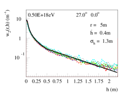
Figure 13: The distribution $w_{2}(r,h)$ for $r=5\,\mathrm{m}$. The full black line represents the fit, the dotted lines are simulation results for different times.

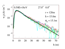
Figure 14: The distribution $w_{2}(r,h)$ for $r=128\,\mathrm{m}$. The full black line represents the fit, the dotted lines are simulation results for different times.

we show the fits of $w_{2}$ together with Monte Carlo simulation results for different times. In fig. 15, we show the fitted $w_{2}$ curves for three different values of $r$, conveniently plotted as $h\,w_{2}$ versus $h/\bar{h}$, where one clearly sees the evolution of the shape with $r$.

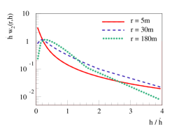
Figure 15: The distribution $w_{2}(r,h)$ for $r=5\,\mathrm{m}$(full line), $r=30\,\mathrm{m}$ (dashed line), and $r=180\,\mathrm{m}$ (dotted line).

The reason to switch between $w_{2}^{\mathrm{MGD}}$ and $w_{2}^{\mathrm{IGD}}$ at $r_{0}=20$ m becomes clear from figures 13 through 15. From figure 15 it can be seen clearly that the particle distribution as obtained from the Monte-Carlo simulations behaves quite differently close to the shower axis as compared to the distribution at large distances. This different behavior requires the use of different fit-functions in both regimes. At large distances from the core, the parametrization of $w_{2}^{\mathrm{MGD}}$ reproduces the MC result accurately. At small distances, it is important to have a smooth parametrization without jumps in the first derivatives, which is the case when using $w_{2}^{\mathrm{IGD}}$.

The above fit function $w_{2}^{\mathrm{IGD}}$ leads to a delta-peak at $r=0$. To still obtain numerical stability, a cut-off for the values $K^{\prime}$ and $H_{5}$ is introduced such that the width of $w_{2}^{\mathrm{IGD}}$ is 1 mm. Since most of the particles are located within $r=\delta x^{\perp}=1$ m from the shower axis, the path difference between signals emitted at this distance on both sides of the shower axis acts as the important length scale in this regime. We estimate this path difference $\delta R$ for a constant index of refraction equal to $n=1.0003$ : we have $\delta{R}\approx\frac{\partial R}{\partial x^{\perp}}\delta x^{\perp}\approx\sqrt{n^{2}\beta^{2}-1}\delta x^{\perp}\approx 3$ cm. Here we use that at the Cherenkov time (critical time for $h=0$), we have $R^{0}=n\beta x^{||}$, and $x_{c}^{||}=\sqrt{n^{2}\beta^{2}-1}x_{c}^{\perp}$ arena . So a cut-off of $w_{2}^{\mathrm{IGD}}\approx 1$ mm should give stable results. This has been tested numerically.

IV Time signals

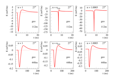
Figure 16: The $y$ component of the geomagnetic contribution to the electric field as a function of the observer time $t$ in ns, for an observer distance of 112 m (upper panel) and 448 m (lower panel) We compare different options for the index of refraction $n$, namely $n=1$(left), $n=n_{\mathrm{GD}}$(middle), and $n=1.0003$(right).

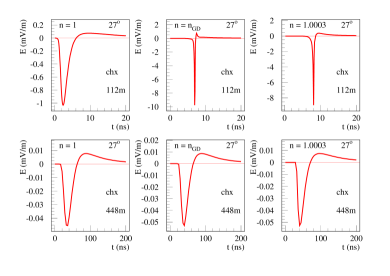
Figure 17: The $x$ component of the charge excess contribution to the electric field as a function of the observer time $t$ in ns, for an observer distance of 112 m (upper panel) and 448 m (lower panel) We compare different options for the index of refraction $n$, namely $n=1$(left), $n=n_{\mathrm{GD}}$(middle), and $n=1.0003$(right).

As already said, the eqs. (17,18) are evaluated employing the EVA 1.0 package, which provides the weights $w$, the currents $J$, the denominators $\tilde{R}V$, and the integration procedures, as discussed in the previous chapter. We first consider the same “reference shower” (initial energy of $5\cdot 10^{17}$eV, inclination $27^{o}$) already discussed there. We will distinguish between the geomagnetic contribution (caused by the currents due to the geomagnetic field) and the contributions due to charge excess. In figs. 16 and 17, we show the results for the two contributions, for two different observer positions: 112 and 448 meters to the south of the impact point. We compare the realistic scenario ($n=n_{\mathrm{GD}})$ with the two “limiting cases” $n=1$ and $n=1.0003$. One can clearly see big differences between the three scenarios, up to a factor of ten in width and magnitude. We also see, even in the realistic case ($n=n_{\mathrm{GD}})$, the appearance of “Cherenkov-like” behavior, with very sharp peaks.

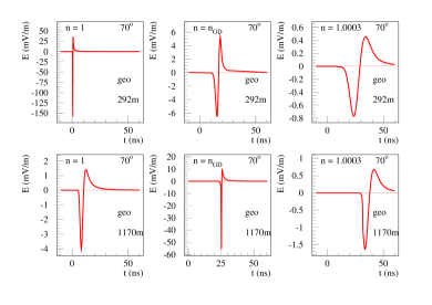
Figure 18: Same as fig 16, but here we consider a more inclined shower.

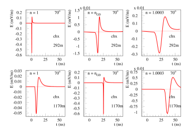
Figure 19: Same as fig 17, but here we consider a more inclined shower.

In figs. 18 and 19, we consider a more inclined shower ($70^{o}$), for two different observer positions: 292 and 1170 meters to the south of the impact point. The differences between the realistic case ($n=n_{\mathrm{GD}})$ and the two “limiting cases” is even bigger: more than a factor of 100 in width and magnitude!

V Geomagnetic Cherenkov radiation

As shown in the last chapter, a realistic treatment of the index of refraction in the atmosphere seems to be very crucial for the forms of the electromagnetic pulses. Can this be seen in experiments? What exactly should one look for?

To answer these questions we will discuss in the following frequency spectra. As shown in chapter II, the fields are sums of terms of the form (up to factors)

$$\int\,dV\mathrm{\>pancake}\>\times\>\mathrm{currents}\>\times\left(\frac{dt^{*}}{dt}\right),$$ (30)

where “currents” and “pancake” refer to respectively the pointlike currents and the current distributions in the pancake, or its derivatives. The quantity $dV$ is a pancake volume element. The currents and the “Cherenkov term” $dt^{*}/dt$ are taken at the retarded time $t^{\prime}=t^{*}$, for a given observer time and position. Let us consider the evolution of an air shower in time $t^{\prime}$. The currents are essentially proportional to the electron number $N_{e}(t^{\prime})$ of the shower, the so-called “profile”. We define $t{}_{P}^{*}$ to be an emission time (retarded time) corresponding to the profile maximum, also referred to as shower maximum. Another important quantity is the Cherenkov time $t_{C}^{*}$, corresponding to the time where $dt^{*}/dt$ becomes singular.

The electric field contains actually terms governed by the derivatives of the currents, and therefore by the derivative of the profile. We consider therefore the expression “shower maximum” to represent the actual maximum of the profile or of its derivative.

A strong signal is expected when the two times $t{}_{P}^{*}$ and $t_{C}^{*}$ coincide. Such a situation is shown in fig. 20,

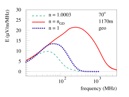
Figure 20: Fourier transform of geomagnetic component of the 70 degrees inclined shower observed at 1170 meters from the shower core. We plot the modulus of the Fourier transform.

where we plot the Fourier spectrum for the geomagnetic component of the electromagnetic field for the $70$ degrees inclined shower discussed in the previous chapter, with an initial energy of $5\cdot 10^{17}$eV, and an observer positioned at a distance of $d=1170$ m to the east of the impact point of the shower, corresponding to an impact parameter $b$ of around $400$ m. At this distance the shower maximum occurs at the Cherenkov time for a realistic index of refraction. The realistic case ($n=n_{GD}$) contains very high frequency components up to several GHz as one would expect from the sharp peak in figure 18. The two limiting cases peak at lower frequencies below $100$ MHz.

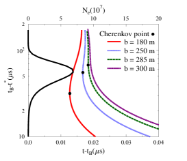
Figure 21: The shower profile as a function of $t^{*}$ (black line) and the retarded times $t^{*}$ as a function of the observer time $t$, relative to the time of closest approach $t_{B}$ (red, blue, and magenta curves). The “Cherenkov points” correspond to the Cherenkov times (where $dt^{*}/dt$ is singular).

In the following, we discuss some very interesting features by taking the example of a $60$ degrees inclined shower with an initial energy of $10^{17}$ eV, moving from west to east, in a magnetic field of strength 24.3$\mu\mathrm{T}$ and an inclination $\alpha$ of $54^{o}$ (Auger site). The observer is positioned to the east of the impact point. We will use the impact parameter rather than the horizontal distance (as in the examples before) to characterize the observer position.

In fig. 21, we plot the shower profile $N_{e}$ as a function of the retarded time $t^{*}$, together the retarded times $t^{*}$ as a function of the observer time $t$, for three different choices of the impact parameter. For large values of $b$ (above 285m), like the case of 300 meters (magenta curve), there is no Cherenkov time, the function $t^{*}(t)$ is single valued, the derivative is always finite. We have “normal” emission, coming from around the the maximum of the profile corresponding to $t^{\prime}=t_{P}^{*}$, see fig. 22. The form of the time signal is determined by the profile, we expect maximum frequencies around few hundred MHz, as confirmed by the calculation shown in fig. 25. At impact parameters smaller than 285 meters, the function $t^{*}(t)$ starts to become double valued, so we we start observing a Cherenkov time. At 250 meters, the Cherenkov time coincides with the shower maximum, we have

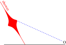
Figure 22: The observer $O$ receives “normal emission” from around the shower maximum.

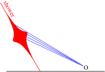
Figure 23: The observer $O$ receives “Cherenkov emission” from around the shower maximum.

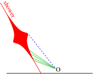
Figure 24: The observer $O$ receives both “normal emission” from around the shower maximum and “Cherenkov emission” from later times.

Cherenkov emissions from around the shower maximum. This means that due to $dt^{*}/dt=\infty$, the emissions from a broad region around the maximum will be “compressed” and arrive almost at the same time at the observer, as sketched in fig. 23. This leads to a strong and very short signal. Since the singularity is integrated over, as explained in chapter II, the actual width of the same signal is determined by the current distributions in the pancake, and we expect frequencies around a GHz, as confirmed by the calculation shown in fig. 25.

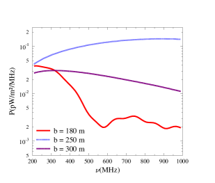
Figure 25: Flux densities for radio emission from a $10^{17}$ eV energy shower at 60^o zenith angle for impact parameters of 180, 250, and 300 meters.

If the observer is even closer to the shower, for example at an impact parameter of 180 meters, we still have a Cherenkov time, but this time is now significantly later than the shower maximum time (see the dot on the red curve in fig. 21). Here we may have a very interesting situation: the observer may receive “normal” emission from around the shower maximum, but at the same time he may receive a significant contribution from much later, around the Cherenkov time, which again due to the Cherenkov effect (signal compression) will be relatively strong and short (high frequency, order of GHz). This situation is sketched in fig. 24. The calculations in fig. 25 show (as expected) two distinct peaks, one at small frequencies due to the normal emission from the shower maximum, and a second peak at high frequencies due to Cherenkov emission at much later times.

So our approach predicts not only high frequency components due to the geomagnetic Cherenkov effect, but in addition a double peak structure which reflects the simultaneous reception of signals from very different positions of the shower: “normal” emissions from around the maximum, and Cherenkov emission from much later times.

VI Comparing to data

This geomagnetic Cherenkov radiation might have been observed by the ANITA-collaboration anita , where pulses have been measured in the $200$-$1200$ MHz band. Furthermore, since these high frequency components occur only at the Cherenkov distance, upon applying a high-pass filter a clear Cherenkov ring should become visible in the LDF. The radius of this ring contains direct information of the shower maximum and thus the chemical composition of the original cosmic ray. New experiments at the Pierre Auger observatory auger1 ; auger2 , and LOFAR lofar should be able to measure the LDF in more detail, where first hints of "Cherenkov-like" effects might have been observed lopes ; lofar2 .

The key result of our present work is the prediction of a sizable power emitted at higher frequencies, and a possible double peak structure with one peak at high frequencies. There exist only few observations where the spectrum over a large frequency range has been measured. A good example was published recently by the ANITA collaboration Hoover10 , showing the summed power of two cosmic-ray events for the range of 300-900 MHz.

In this measurement no indication is given of the arrival direction and the energy of the initiating cosmic ray, only that it most probably came from a relatively large zenith angle. The azimuth angle is unknown. Therefore also the air density along the path of the air shower is unknown, as well as its orientation with respect to the magnetic field. All this makes any quantitative comparison impossible. To get at least a qualitative understanding, we compare the data with the result of a simulation for a cosmic-ray at a zenith angle of $60^{\circ}$ , moving from west to east, in a magnetic field corresponding to the Auger site, with an observer east to the impact point, for various impact parameters $b$ – the same situation as discussed in the previous chapter (changing the energy and the arrival direction of the cosmic ray will not change the qualitative discussion).

In fig. 26,

Figure 26: The predicted flux densities for radio emission from a $10^{17}$ eV energy shower at 60^o zenith angle for various impact parameters $b$ are compared to the data for the sum of two events as measured by the ANITA balloon mission Hoover10 , where the data are taken from fig. 3 of that publication.

we compare the data with our simulation results. We show blue curves corresponding to 350 - 225 m, from bottom to top for the leftmost value. The red curves refer to 200 - 180m, from top to bottom.

From the discussion of the last chapter, we easily understand the different theoretical curves: for large impact parameters 350, 325, 300m) we have the situation corresponding to fig. 22: normal emission from around the shower maximum dominates. For impact parameters around 250 meters, we have Cherenkov emission from around the shower maximum, as in fig. 23, we get strong signals at large frequencies (GHz). Then finally below 200 meters, we have the situation sketched in fig. 24: a double peak structure due to simultaneously arriving signals from very different positions of the shower: “normal” emissions from around the maximum, and Cherenkov emission from later times.

Although energy and inclination of the measured showers are unknown, it is nevertheless clear that the data show a structure similar to the transition region towards a double peak behavior, as predicted in our calculations shown in fig. 26.

VII Summary

We presented a realistic calculation of coherent electro-magnetic radiation from air showers initiated by ultra-high energy cosmic rays. The underlying currents are obtained from three-dimensional Monte Carlo simulations of air showers in a realistic geo-magnetic field. We take into account the correct shape of the particle distribution in a shower at a given time. The numerical procedures – simulations, fitting procedures, convolutions, referred to as EVA 1.0 – have been discussed. We showed the importance of a correct treatment of the index of refraction in air, given by the law of Gladstone and Dale: using the correct index of refraction $n_{\mathrm{GD}}$ gives very different results compared to a simplified treatment using a constant index, with differences in width and magnitude up to a factor of 100. The new treatment leads in particular to important emission at high frequencies (GHz). In certain cases, double peak structures are predicted, due to signals arriving simultaneously from different positions of the shower: “normal” emissions from around the maximum, and Cherenkov emission from later times.

Appendix A Some derivatives

Theorem: The quantity $h_{k}$ is a function of $t$ and $x^{\|}$(the transverse coordinates are not considered here). Its derivatives are

$$\frac{d}{d\,ct}h_{k}=-1,\quad\frac{d}{dx^{\|}}h_{k}=1.$$ (31)

The time derivatives of $ct^{*}$ and $\tilde{R}V$ vanish:

$$\frac{d}{d\,ct}ct^{*}=\frac{d}{d\,ct}\tilde{R}V=0.$$ (32)

Proof:

In the following, we do not consider explicitly the transverse coordinates (to be considered constant). The variables of interest are the time $ct\equiv x^{0}$ and the longitudinal coordinate $x^{\|}\equiv z$. We use for any function $f(t,z)$ the notation $\partial^{0}f=\partial f/\partial\,ct$, $\partial^{z}f=-\partial f/\partial z$. For the “total” derivatives, we use $d^{0}f=df/d\,ct$, $d^{z}f=-df/dz$.

We consider for given fixed $h$ the retarded time $t^{*}(t,z-h)$. The retarded time corresponding to a critical time is given as

$$t_{k}^{*}=t^{*}(t_{k},z-h),$$ (33)

with $t_{k}=t_{k}(z-h)$. So we have $t_{k}^{*}=t_{k}^{*}(z-h)$. We have

$$d^{z}t_{k}^{*}=\partial^{0}ct^{*}\,d^{z}t_{k}+\partial^{z}t^{*}.$$ (34)

In the following we make extensively use of definitions and relations from reference klaus1 . For $t=t_{k}$, we have

$$\widetilde{R}V=c(t_{k}-t_{k}^{*})+\tilde{R}_{j}V^{j}|_{t^{*}=t_{k}^{*}}=0.$$ (35)

We compute the derivative $d^{z}$ :

$$\>0\>=d^{z}ct_{k}-d^{z}ct_{k}^{*}+(\bar{g}_{\>j}^{z}-\tilde{V}_{j}d^{z}ct_{k}^{*})V^{j}$$ (36)

$$\quad=d^{z}ct_{k}-(1-\tilde{V}^{j}V^{j})d^{z}ct_{k}^{*}+\bar{V}^{z}$$ (37)

$$\quad=d^{z}ct_{k}-\tilde{V}Vd^{z}ct_{k}^{*}+\bar{V}^{z}$$ (38)

$$\quad=d^{z}ct_{k}-\tilde{V}V(\partial^{0}ct^{*}\,d^{z}ct_{k}+\partial^{z}ct^{*})+\bar{V}^{z},$$ (39)

which leads to (using $\bar{V}^{z}=\bar{V}^{\|}$)

$$d^{z}ct_{k}=\frac{-\bar{V}^{\|}+\tilde{V}V\,\partial^{z}ct^{*}}{1-\tilde{V}V\,\partial^{0}ct^{*}}.$$ (40)

Using

$$\partial^{\alpha}ct^{*}=\frac{\bar{R}^{\alpha}}{\widetilde{R}V},$$ (41)

we get

$$d^{z}ct_{k}=-\frac{\bar{V}^{\|}-\tilde{V}V\,\bar{R}^{\|}/\widetilde{R}V}{1-\tilde{V}V\,\bar{R}^{0}/\widetilde{R}V}.$$ (42)

The time derivative of $h_{k}$ as obtained from its definition is

$$d^{0}h_{k}=\left(d^{z}\,ct_{k}\right)^{-1},$$ (43)

which gives

$$d^{0}h_{k}=-\frac{\widetilde{R}V-\tilde{V}V\,\bar{R}^{0}}{\widetilde{R}V\,\bar{V}^{\|}-\tilde{V}V\,\bar{R}^{\|}}.$$ (44)

Using $\widetilde{R}V=0$, and $\bar{R}^{\|}\approx L=\bar{R}^{0}$, we find

$$d^{0}h_{k}=-1.$$ (45)

The other derivative of $h_{k}$ is trivial:

$$d^{z}h_{k}=-1.$$ (46)

The potential $A$, its denominator $\tilde{R}V$, and also the argument $ct^{*}$of its numerator $J$ are evaluated at the parallel coordinate $x^{\|}-h_{k}+\lambda$, so the total time derivatives are

$$d^{0}=\partial^{0}+d^{0}h_{k}\,\partial^{z},$$ (47)

explicitly

$$d^{0}=\partial^{0}-\partial^{z}.$$ (48)

We get

$$d^{0}ct^{*}=(\partial^{0}-\partial^{z})ct^{*}=\frac{\bar{R}^{0}-\bar{R}^{z}}{\widetilde{R}V}=0,$$ (49)

and with

$$\partial^{\alpha}\tilde{R}V=\bar{V}^{\alpha}-\tilde{V}V\,\partial^{\alpha}ct^{*}$$ (50)

(eq. (22) from klaus1 ), we obtain

$$d^{0}\tilde{R}V=0.$$ (51)

References

- (1) H. Falcke, et al., Nature 435, 313 (2005).
- (2) W. D. Apel, et al., Astropart. Physics 26, 332 (2006).
- (3) D. Ardouin, et al., Astropart. Physics 26, 341 (2006).
- (4) A. Corstanje et al, "LOFAR: Detecting Cosmic Rays with a Radio Telescope", arXiv:1109.5805v1, Contribution to the 32nd International Cosmic Ray Conference (Beijing, China, 11-18 Aug. 2011).
- (5) J. Coppens et al. (Pierre Auger Collaboration), Nucl. Instrum. Methods Phys. Res., Sect. A 604, S41 (2009).
- (6) S. Fliescher et al. (Pierre Auger Coll.), Nucl. Instrum. Methods Phys. Res., Sect. A 662, S124 (2012)
- (7) H. R. Allan, Prog. in Element. part. and Cos. Ray Phys. 10, 171 (1971).
- (8) F.D. Kahn and I.Lerche, Proc. Royal Soc. London A289, 206 (1966).
- (9) N.A. Porter, C.D. Long, B. McBreen, D.J.B Murnaghan and T.C. Weekes, Phys. Lett. 19, 415 (1965).
- (10) J. V. Jelley et al., Nature 205, 327 (1965).
- (11) O. Scholten, K. Werner, and F. Rusydi, Astropart. Phys. 29, 94 (2008).
- (12) K.D. de Vries, A.M. van den Berg, O. Scholten, K. Werner, Astropart. Phys. 34, 267 (2010).
- (13) M. Ludwig and T. Huege, Nucl. Instrum. Methods Phys. Res., Sect. A 662, S164 (2012)
- (14) J. Alvarez-Mu, W.R. Carvalho Jr., E. Zas, arXiv:1107.1189v1
- (15) T. Huege et al., Nucl. Instrum. Methods Phys. Res., Sect. A 662, S179 (2012)
- (16) K. Werner, O. Scholten, Astropart. Phys. 29: 393-411, 2008, arXiv:0712.2517.
- (17) K.D. de Vries, A.M. van den Berg, O. Scholten, K. Werner, Phys.Rev.Lett.107:061101,2011
- (18) G. Bossard, H.J. Drescher, N.N. Kalmykov, S. Ostapchenko, A.I. Pavlov, T. Pierog, E.A. Vishnevskaya, and K. Werner, Phys. Rev. D63, 054030, (2001)
- (19) T. Bergmann R. Engel, D. Heck, N.N. Kalmykov, Sergey Ostapchenko, T. Pierog, T. Thouw, and K. Werner , Astropart. Phys. 26, 420 (2007)
- (20) W. R. Nelson et al., The EGS4 Code System, SLAC report 265, 1985
- (21) K.D. de Vries, O. Scholten, and K. Werner, Nucl. Instrum. Methods Phys. Res., Sect. A 662, S175 (2012)
- (22) ANITA Collab: S. Hoover et al., To be submitted to Phys. Rev. Lett arXiv:1005.0035v2
- (23) W. D. Apel et al. (LOPES Collaboration), Astropart. Phys. 32, 294 (2010).
- (24) A. Horneffer et al. (LOFAR CR-KSP Collaboration), Nucl. Instrum. Methods Phys. Res., Sect. A 617, 482 (2010).
- (25) S. Hoover et al., PRL 105, 151101 (2010)