Polarization of graphene in a strong magnetic field beyond the Dirac cone approximation

Abstract

In this paper we study the excitation spectrum of graphene in a strong magnetic field, beyond the Dirac cone approximation. The dynamical polarizability is obtained using a full $\pi$-band tight-binding model where the effect of the magnetic field is accounted for by means of the Peierls substitution. The effect of electron-electron interaction is considered within the random phase approximation, from which we obtain the dressed polarization function and the dielectric function. The range of validity of the Landau level quantization within the continuum approximation is studied, as well as the non-trivial quantization of the spectrum around the Van Hove singularity. We further discuss the effect of disorder, which leads to a smearing of the absorption peaks, and temperature, which activates additional inter-Landau level transitions induced by the Fermi distribution function.

I Introduction

One of the most remarkable features of graphene is its anomalous quantum Hall effect (QHE), which reveals the relativistic character of the low energy carriers in this material.Novoselov et al. (2005); Zhang et al. (2005) In fact, the linear electronic dispersion of graphene near the neutrality point leads to a relativistic quantization of the electrons’ kinetic energy into non-equidistant Landau levels (LL), with the presence of a zero-energy LL, which is the characteristics spectrum for systems of massless Dirac fermions.Katsnelson (2012); Goerbig (2011) As a consequence, the excitation spectrum and the screening properties in graphene are different from those of a standard two-dimensional electron gas (2DEG) with a quadratic band dispersion, as it may be seen from the polarization and dielectric function in the two cases.Shung (1986); Wunsch et al. (2006); Hwang and Sarma (2007); Roldán et al. (2010a); Pyatkovskiy and Gusynin (2011)

The Coulomb interaction between electrons in completely filled LLs leads to collective excitations and to the renormalization of the electronic properties such as the band dispersion and the Fermi velocity. These issues have been studied both theoreticallyIyengar et al. (2007); Shizuya (2007); Gusynin et al. (2007); Bychkov and Martinez (2008); Roldán et al. (2009); Shizuya (2010); Wu et al. (2011) and experimentally, in the framework of cyclotron resonance experiments.Sadowski et al. (2006); Jiang et al. (2007); Deacon et al. (2007); Henriksen et al. (2010); Faugeras et al. (2011) However, most of the theoretical work has been based on the continuum Dirac cone approximation, which does not apply when high energy inter-LL transitions are probed.Plochocka et al. (2008) In recent experimental realization of “artificial graphene”,Singha et al. (2011) a two-dimensonal nanostructure that consists of identical potential wells (quantum dots) arranged in a honeycomb lattice, the lattice constant ($a\sim 130$ nm) is much larger than the one in graphene ($a_{0}\sim 0.142~{}$nm). This provides a way to study graphene in the ultra-high magnetic field limit, since a perpendicular magnetic field in “artificial graphene” correspondes to an effective field which is $(a/a_{0})^{2}\sim 8\times 10^{5}$ times larger than in graphene. Furthermore, the recently developed techniques of chemical dopingMcChesney et al. (2010) and electrolytic gating Efetov and Kim (2010) have enabled doping graphene with ultrahigh carrier densities, where the band structure is no longer Dirac-like and one should take into account the full $\pi$-band structure including the Van Hove singularities (VHS).

In this paper, we present a complete theoretical study of the density of states (DOS), the polarizability and dielectric function of graphene in a strong magnetic field, calculated from a $\pi$-band tight-binding model. The magnetic field has been introduced by means of a Peierls phase,Luttinger (1951); Katsnelson (2012) and the effect of long range Coulomb interaction is accounted for within the random phase approximation (RPA). Our method allows us to study the effect of temperature, which leads to the activation of additional inter-LL transitions. We also study the effect of disorder in the spectrum, which leads to a smearing of the resonance peaks.

II Description of the Method

In this section we summarize the method used in the numerical calculation of the polarizability of graphene in the QHE regime. A monolayer of graphene consists of two triangular sublattices of carbon atoms with an inter-atomic distance of $a\approx 1.42$ Å. By considering only first neighbor hopping between the $p_{z}$ orbitals, the $\pi$-band tight-binding Hamiltonian of a graphene layer is given by

$$H=-\sum_{\langle i,j\rangle}(t_{ij}a_{i}^{\dagger}b_{j}+\mathrm{h.c.})+\sum_{i}v_{i}c_{i}^{\dagger}c_{i},$$ (1)

where $a_{i}^{\dagger}$ ($b_{i}$) creates (annihilates) an electron on sublattice A (B) of the graphene layer, and $t_{ij}$ is the nearest neighbor hopping parameter, which oscillates around its mean value $t\approx 3$ eV.Castro Neto et al. (2009) The second term of $H$ accounts for the effect of an on-site potential $v_{i}$, where $n_{i}=c_{i}^{\dagger}c_{i}$ is the occupation number operator. For simplicity, we omit the spin degree of freedom in Eq. (1), which contributes only through a degeneracy factor. In our numerical calculations, we use periodic boundary conditions. The effect of a perpendicular magnetic field $\mathbf{B}=B{\hat{\mathbf{z}}}$ is accounted by means of the Peierls substitution, which transforms the hopping parameters according toLuttinger (1951)

$$t_{ij}\rightarrow t_{ij}\exp{\left(i\frac{2\pi}{\Phi_{0}}\int_{\mathbf{R}_{i}}^{\mathbf{R}_{j}}\mathbf{A}\cdot d\mathbf{l}\right)},$$ (2)

where $\Phi_{0}=hc/e$ is the flux quantum and $\mathbf{A}$ is the vector potential, e. g. in the Landau gauge $\mathbf{A}=(-By,0,0)$. We will calculate the DOS and the polarization function of the system by using an algorithm based on the evolution of the time-dependent Schrödinger equation. For this we will use a random superposition of all basis states as an initial state $|\varphi\rangle$ (see e. g. Refs.Hams and De Raedt, 2000; Yuan et al., 2010)

$$\left|\varphi\right\rangle=\sum_{i}a_{i}c_{i}^{\dagger}c_{i}\left|0\right\rangle,$$ (3)

where $a_{i}$ are random complex numbers normalized as $\sum_{i}\left|a_{i}\right|^{2}=1$. The DOS, which describes the number of states at a given energy level, is then calculated as a Fourier transform of the time-dependent correlation functions

$$d(\epsilon)=\frac{1}{2\pi}\int_{-\infty}^{\infty}e^{i\epsilon\tau}\langle\varphi|e^{-iH\tau}|\varphi\rangle d\tau,$$ (4)

with the same initial state defined in Eq. (3). The dynamical polarization function can be obtained from the Kubo formulaKubo (1957)

$$\Pi\left(\mathbf{q},\omega\right)=\frac{i}{V}\int_{0}^{\infty}d\tau e^{i\omega\tau}\left\langle\left[\rho\left(\mathbf{q},\tau\right),\rho\left(-\mathbf{q},0\right)\right]\right\rangle,$$ (5)

where $V$ denotes the volume (or area in 2D) of the unit cell, $\rho\left(\mathbf{q}\right)$ is the density operator given by

$$\rho\left(\mathbf{q}\right)=\sum_{i}c_{i}^{\dagger}c_{i}\exp\left(i\mathbf{q\cdot r}_{i}\right),$$ (6)

and the average is taken over the canonical ensemble. For the case of the single-particle Hamiltonian, Eq. (5) can be written asYuan et al. (2010)

$$\Pi\left(\mathbf{q},\omega\right)=-\frac{2}{V}\int_{0}^{\infty}d\tau e^{i\omega\tau}$$

$$\times\text{Im}\left\langle\varphi\right|n_{F}\left(H\right)e^{iH\tau}\rho\left(\mathbf{q}\right)e^{-iH\tau}\left[1-n_{F}\left(H\right)\right]\rho\left(-\mathbf{q}\right)\left|\varphi\right\rangle,$$

where

$$n_{F}\left(H\right)=\frac{1}{e^{\beta\left(H-\mu\right)}+1}$$ (8)

is the Fermi-Dirac distribution operator, $\beta=1/k_{B}T$ where $T$ is the temperature and $k_{B}$ is the Boltzmann constant, and $\mu$ is the chemical potential. In the numerical simulations, we use units such that $\hbar=1$, and the average in Eq. (II) is performed over the random superposition Eq. (3). The Fermi-Dirac distribution operator $n_{F}\left(H\right)$ and the time evolution operator $e^{-iH\tau}$ can be obtained by the standard Chebyshev polynomial decomposition.Yuan et al. (2010)

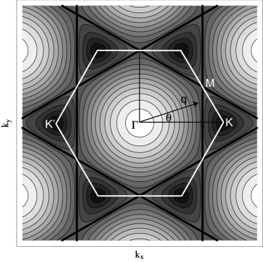
Figure 1: Constant energy contours obtained from the band dispersion Eq. (13). The thick black lines correspond to dispersion at the VHS $|\epsilon|=t$. Notice that the CEC are centered around the Dirac points for $|\epsilon|<t$ and around $\Gamma$ for $|\epsilon|>t$. For illustrative reasons, the hexagonal BZ is shown in white. For undoped graphene, the valence and conduction bands touch each other at the vertices of the hexagon, the so called Dirac points (K and K’). The Van Hove singularity lies at the M point, and we have defined $\theta$ as the angle between the wave-vector $q$ and the $k_{x}$-axis.

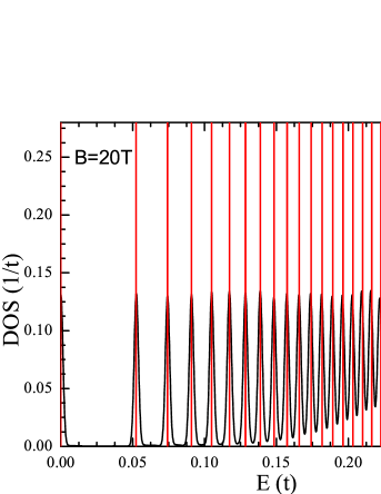
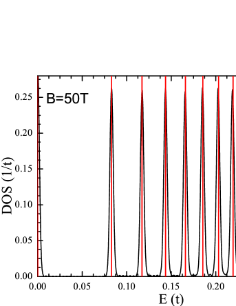
Figure 2: Left: DOS of a monolayer of graphene in a magnetic field, for two different values of $B$. Right: zoom of the low energy region of the spectrum. The red vertical lines indicate the position of the LLs in the continuum Dirac cone approximation, Eq. (19). We have used a sample made of 4096$\times$4096 atoms.

Long range Coulomb interaction is considered in the RPA, leading to a dressed particle-hole polarization

$$\chi\left(\mathbf{q},\omega\right)=\frac{\Pi\left(\mathbf{q},\omega\right)}{\mathbf{1}-V\left(q\right)\Pi\left(\mathbf{q},\omega\right)},$$ (9)

where

$$V\left(q\right)=\frac{2\pi e^{2}}{\kappa q}$$ (10)

is the Fourier component of the Coulomb interaction in two dimensions, in terms of the background dielectric constant $\kappa$. Furthermore, the dielectric function of the system is calculated as

$$\mathbf{\varepsilon}\left(\mathbf{q},\omega\right)=1-V\left(q\right)\Pi\left(\mathbf{q},\omega\right).$$ (11)

The collective modes lead to zeroes of $\varepsilon(\mathbf{q},\omega)$, and their dispersion relation is defined from

$$\mathrm{Re}~{}\varepsilon(\mathbf{q},\omega_{pl})=1-V(q)\Pi(\mathbf{q},\omega_{pl})=0,$$ (12)

which leads to poles in the response function (9). The technicalities about the accuracy of the numerical results have been discussed elsewhere.Hams and De Raedt (2000); Yuan et al. (2010, 2011a) Here we just mention that the efficiency of the method is mainly determined by three factors: the time interval of the propagation, the total number of time steps, and the size of the sample. The method is more efficient in the presence of strong magnetic fields. Because for weak fields (e.g., $B<1$ T) the energy difference between LLs become very small, this makes that the total number of time steps and the size of the sample have to be large enough to provide the necessary energy resolution in the numerical simulation.

III Density of states and excitation spectrum

In this section we study the DOS and the excitation spectrum of a graphene layer in a magnetic field, neglecting the effect of disorder and electron-electron interaction. The $B=0$ dispersion relation of the $\pi$ bands obtained from a tight-binding model with nearest-neighbor hopping between the $p_{z}$ orbitals is

$$\epsilon(\mathbf{k})=\lambda t|\phi_{\mathbf{k}}|$$ (13)

where $\lambda=\pm 1$ is the band index and

$$\phi_{\mathbf{k}}=1+2e^{i3k_{x}a/2}\cos\left(\frac{\sqrt{3}}{2}k_{y}a\right).$$ (14)

The band dispersion Eq. (13) consists of two bands that touch each other in the vertices of the hexagonal Brilloin zone (BZ) (Fig. 1), which are the so called Dirac points. In the absence of longer range hopping terms, the band structure is electron-hole symmetric, and the constant energy contours (CEC) obtained from Eq. (13) are shown in Fig. 1. For undoped graphene ($\mu=0$), which is the band filling that we will consider all along this paper, the Fermi surface consists of just six points at the vertices of the BZ. In this case, the low energy excitations can be described by means of an effective theory obtained from an expansion of the dispersion Eq. (13) around the K points. This leads to an approximate dispersion $\epsilon(\mathbf{k})\approx\lambda v_{F}k$, where $v_{F}=3ta/2$ is the Fermi velocity.

If we now consider the effect of a perpendicular magnetic field, the Landau quantization of the kinetic energy leads to a set of LLs, which can be described from the semiclassical conditionShoenberg (1984); Katsnelson (2012)

$$S(C)=\frac{2\pi}{l_{B}^{2}}\left(n+\frac{1}{2}-\frac{\Gamma(C)}{2\pi}\right)$$ (15)

where

$$S(C)=\underset{\epsilon\left(k_{x},k_{y}\right)\leq\text{ }\epsilon_{n}}{\int\int}dk_{x}dk_{y}$$ (16)

is the area enclosed by the cyclotron orbit $C$ in momentum space [for circular orbits $S(C)$ is just $\pi k^{2}$], $l_{B}=\sqrt{\hbar c/eB}$ is the magnetic length, $n$ is the LL index and $\Gamma(C)$ is the Berry phase. In graphene, as we will discuss in the next section, $\Gamma(C)=\pi$ for orbits around the K and K’ points, and 0 for orbits around the $\Gamma$ point.Fuchs et al. (2010) From the energy dependence of $S(C)$ one can calculate the energy of the Landau levels as

$$\epsilon_{n}=S^{-1}\left(\frac{2\pi}{l_{B}^{2}}\left[n+\frac{1}{2}-\frac{\Gamma(C)}{2\pi}\right]\right),$$ (17)

where $S^{-1}(x)$ is the inverse function to $S(x)$. Using Eq. (17), it is easy to check that the LL quantization corresponding to a low energy parabolic band $\epsilon(k)=k^{2}/2m_{b}$ (where $m_{b}$ is the effective mass) with a $\Gamma(C)=0$ Berry phase, is $\epsilon_{n}=\omega_{c}(n+1/2)$, where $\omega_{c}=eB/m_{b}$ is the cyclotron frequency. On the other hand, a linearly dispersing band as the one for graphene leads to a LL quantization around the Dirac points as

$$\epsilon_{\lambda,n}=\lambda\epsilon_{n}=\lambda\frac{v_{F}}{l_{B}}\sqrt{2n}\propto\sqrt{Bn}.$$ (18)

Figure 3: DOS obtained from Eq. (4) at $B=500$T. The insets show a zoom of the DOS around the VHS $|\epsilon|\approx t$ and at $|\epsilon|\approx 2.5t$.

III.1 Density of states

The DOS close to the Dirac point can be approximated byCastro Neto et al. (2009)

$$d_{\mathrm{Dirac}}(\epsilon)\approx\frac{2A_{c}}{\pi}\frac{|\epsilon|}{v_{F}^{2}}$$ (19)

where $A_{c}=3\sqrt{3}a^{2}/2$ is the unit cell area. In Fig. 2 we show the DOS for two different values of the magnetic field. The black line corresponds to the numerical tight-binding result obtained from Eq. (4). Near $\epsilon=0$ we notice the presence of a zero energy LL surrounded by a set of LLs whose separation decreases as the energy increases, leading to a stacking of the LLs as we move away from the Dirac points. The presence of a finite broadening in these LLs is due to the energy resolution of the numerical simulations, which is limited by the number of atoms used in the calculation, as well as the total number of time steps, which determines the accuracy of the energy eigenvalues. In order to check the range of validity of the continuum approximation, in the right-hand side of Fig. 2 we show a zoom of the positive low energy part of the DOS for the two values of $B$, comparing the DOS obtained with the full $\pi$-band tight-binding model Eq. (4) [black lines] to the Dirac cone approximation of Eq. (19) [vertical red lines]. Contrary to multi-layer graphenes, for which trigonal warping effects are important at rather low energies,Yuan et al. (2011b) we see that the deviations of the LL positions in the continuum approximation Eq. (19) with respect to the full $\pi$-band model are weak even at energies of the order of $\epsilon\sim 0.3t\sim 1$eV, in agreement with magneto-optical transmission spectroscopy experiments.Plochocka et al. (2008)

A much less investigated issue is the effect of the magnetic field on the DOS around the VHS $|\epsilon|\approx t$. For illustrative reasons we show in Fig. 3 the numerical results for the DOS of a graphene layer at an extremely high magnetic field of $B=500$T. At this energy the LL quantization is highly nontrivial because of the saddle point in the band structure at which there is a transition from CECs encircling the Dirac points, to CECs encircling the $\Gamma$ point, as it can be seen in Fig. 1. Because in the semiclassical limit, the cyclotron orbits in reciprocal space follow the CECs, we have that at the saddle point there is a change in the topological Berry phase $\Gamma(C)$ from $\Gamma(C)=\pm\pi$ for orbits encircling the Dirac points ($|\epsilon|<t$) to $\Gamma(C)=0$ for orbits encircling the $\Gamma$ point ($|\epsilon|>t$).Fuchs et al. (2010) The different character of the cyclotron orbits at both sides of the saddle point leads to two series of LLs, with different cyclotron frequencies $\omega_{c}=eB/m_{b}$, that merge at the VHS, as it may be seen in the left-hand side inset of Fig. 3. Because of the effective mass $m_{b}$ below the VHS is larger than the one above it (the band below the saddle point is flatter than above it), the cyclotron frequencies are also different $\omega_{c}(|\epsilon|<t)<\omega_{c}(|\epsilon|>t)$, and consequently the LLs are more separated for $|\epsilon|>t$ than for $|\epsilon|<t$. The possibility of placing the chemical potential at the VHS would bring the chance of studying highly anomalous inter-LL transitions, due to the different separation of the LLs above and below the VHS. Finally, at an even higher energy, the LL quantization is quite similar to that of a 2DEG with a parabolic dispersion, with a set of roughly equidistant LLs, as it may be seen in the right-hand side inset of Fig. 3 for $|\epsilon|\approx 2.5t$. However, we emphasize that for realistic values of magnetic field, the LL quantization in graphene is inappreciable in this range of energies, and the DOS for energies $|\epsilon|\gtrsim 0.7t$ is similar to the DOS at $B=0$,Yuan et al. (2010) as it may be seen in Fig. 2.

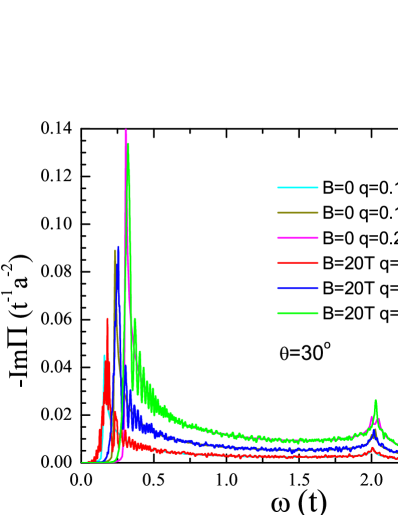
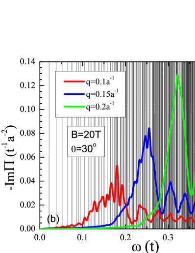
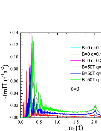
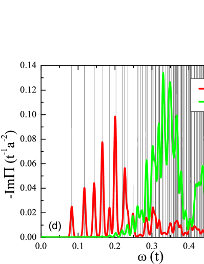
Figure 4: $-\mathrm{Im}\Pi(\mathbf{q},\omega)$ for different values of wave-vector $q$ and strength of the magnetic field $B$. The angle $\theta$ defines the orientation of the wave-vector in the Brilloin zone (see Fig. 1). Plots (a) and (c) show the polarization in the whole energy range. For comparison we show the polarization at $B=0$. In plots (b) and (c) we show the low energy part of the spectrum. The vertical black lines signal the energy of the particle-hole processes expected from Eq. (20).

III.2 Particle-hole excitation spectrum

The particle-hole excitation spectrum (PHES) for non-interacting electrons, which is the part of the $\omega-\mathbf{q}$ plane where $\mathrm{Im}\Pi(\mathbf{q},\omega)$ is non-zero, defines the region of the energy-momentum space where particle-hole excitations are allowed. For undoped graphene ($\mu=0$), the particle-hole excitations correspond to inter-band transitions across the Dirac points. In Fig. 4 we show $-\mathrm{Im}\Pi(\mathbf{q},\omega)$ for different values of wave-vector and magnetic field. Two different orientations of $\mathbf{q}$ are shown, namely along the $\Gamma$-M and $\Gamma$-K directions. First, due to the low energy linear dispersion relation and to the effect of the chirality factor (or wave-function overlap) that suppresses backscattering, we observe that the strongest contribution to the polarization is concentrated around $\omega\approx v_{F}q$. In fact, at $B=0$ it was shownGonzález et al. (1994) that $\mathrm{Im}\Pi(\mathbf{q},\omega)\sim q^{2}(\omega^{2}-v_{F}^{2}q^{2})^{-1/2}$, which implies an infinite response of relativistic non-interacting electrons in graphene at the threshold $\omega=v_{F}q$. The main difference of the PHES at finite magnetic field with respect to its $B=0$ counterpart in this low energy range, is that in the $B\neq 0$ case $\Pi(\mathbf{q},\omega)$ presents a series of peaks of strong spectral weight, due to the LL quantization of the kinetic energy, that we will discuss in more detail below. We notice that, for the realistic values of magnetic field used in Fig. 4, the spectrum at finite magnetic field roughly coincides with the the one at $B=0$ at high energies. This is due to the almost negligible effect of the magnetic field on the DOS at energies $|\epsilon|\gtrsim 0.7t$ for $B\lesssim 50$T, as we saw in the previous section. This part of the spectrum is dominated, as in the $B=0$ case,Stauber et al. (2010); Yuan et al. (2011a) by a peak of $\mathrm{Im}\Pi(\mathbf{q},\omega)$ around $\omega\approx 2t$, which is due to particle-hole transitions between states of the Van Hove singularities of the valence and the conduction bands at $\epsilon\approx-t$ and $\epsilon\approx t$ respectively.

However, the low energy part of the spectrum is completely different to its zero magnetic field counterpart, and it is dominated by a series of resonance peaks at some given energy values. For the undoped case studied here, the possible excitations correspond to inter-LL transitions of energy $\omega_{n,n^{\prime}}=\epsilon_{n^{\prime}}+\epsilon_{n}$, where $n^{\prime}$ is the LL index of the particle in the conduction band ($\lambda=+1$) and $n$ is the LL index of the hole in the valence band ($\lambda=-1$). In the continuum approximation, they have an energy

$$\omega_{n,n^{\prime}}=\sqrt{2}(v_{F}/l_{B})(\sqrt{n^{\prime}}+\sqrt{n}).$$ (20)

The energy corresponding to each of these transitions is indicated by a black vertical line in Fig. 4(b) and (d), where we show a zoom of $-\mathrm{Im}\Pi(\mathbf{q},\omega)$ that corresponds to the low energy LL transitions about the Dirac points. Notice that, in contrast to a standard 2DEG with a parabolic dispersion and equidistant LLs, the relativistic quantization of the energy band in graphene makes that in a fixed energy window at high energies, there are more possible inter-LL excitations from the level $n$ in the valence band to the level $n^{\prime}$ in the conduction band, than at low energies. As a consequence, there is a stacking of neighboring LL transitions as we increase the energy of the excitations, which manifests itself in a continuum of possible inter-LL transitions from a given energy, which for the case of Fig. 4(b) at $B=20$T is $\omega/t\gtrsim 0.25$.

Contrary to what one can naively expect, only at very strong magnetic fields and for small values of $\omega$ and $q$, the peaks of $-\mathrm{Im}\Pi(\mathbf{q},\omega)$ occur at the energies given by Eq. (20). In fact, we can see in Fig. 4(d) that for $B=50$T and for the smaller value of $q$ shown (red line), the peaks of $-\mathrm{Im}\Pi(\mathbf{q},\omega)$ match very well the energies for the inter-LL transitions given by Eq. (20). However, at weaker magnetic fields and/or larger wave-vectors, the peaks of the polarization function do not coincide any more with every of the inter-LL transitions given by Eq. (20). In fact, there is a series of peaks of $\mathrm{Im}\Pi(\mathbf{q},\omega)$, corresponding to regions of the PHES of high spectral weight, which can be understood from the form of the wavefunctions of the electron and the hole that overlap to form an electron-hole pair. A detailed discussion about the structure of the PHES in graphene in comparison with a 2DEG can be found in Ref. Roldán et al., 2010a. Here we just remember that the modulus of the LL wavefunction, due to the zeros of Laguerre polynomials, presents a number of nodes that depend on the LL index $n$. On the other hand, the existence of an electron-hole pair will be possible if there is a finite overlap of the electron and hole wavefunctions, which will define the form factor for graphene in the QHE regime, $\mathcal{F}_{n,n^{\prime}}(\mathbf{q})$. Because the node structure of the single-particle wavefunctions will be transfered to $|\mathcal{F}_{n,n^{\prime}}(\mathbf{q})|^{2}$, all together will lead to a highly modulated spectral weight in the PHES, as it is seen in Fig. 4(b) and (d).

IV Collective modes

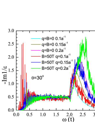
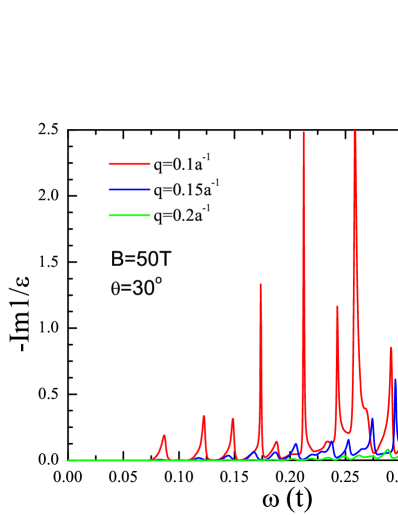
Figure 5: (a) Loss function $-\mathrm{Im}~{}1/\varepsilon(\mathbf{q},\omega)$ in the RPA, for different values of wave-vector. The results for graphene in a magnetic field of $B=50$T are compared to the $B=0$ case. (b) Zoom of the low energy part of the spectrum.

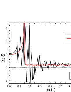
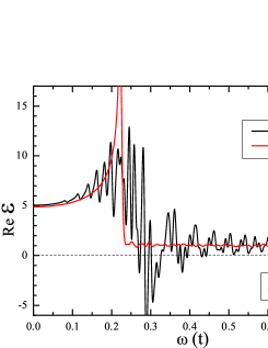
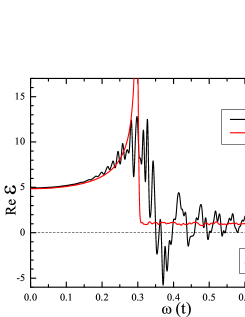
Figure 6: $\mathrm{Re}~{}\varepsilon(\mathbf{q},\omega)$ for $B=0$ (red lines) and $B=50$T (black lines), for the values of the wave-vectors used in Fig. 5.

In the previous section we have discussed the excitation spectrum in the absence of electron-electron interaction. In this section we include in the problem the effect of long range Coulomb interaction. The polarization and dielectric functions are calculated within the RPA, Eqs. (9) and (11). Within this framework, the existence of collective excitations will be identified by the zeros of the dielectric function or equivalently by the divergences of the loss function $-\mathrm{Im}[1/\epsilon(\mathbf{q},\omega)]$, which is proportional to the spectrum measured by Electron Energy Loss Spectroscopy (EELS).Eberlein et al. (2008) In Fig. 5 we show the loss function of graphene in a magnetic field, as compared to the one at $B=0$. At $B=0$ the main structure is the broad peak at $\omega\sim 2t$, associated to the $\pi$-plasmon.Yuan et al. (2011a) When the graphene layer is subjected to a strong perpendicular magnetic field, $\mathrm{Im}[1/\varepsilon(\mathbf{q},\omega)]$ presents a series of prominent peaks at low frequencies, associated to collective modes in the QHE regime, as it may be seen in Fig. 5(b). Similarly to the single-particle case discussed in Sec. III.2, the strength of the peak is determined by the Coulomb matrix elements $V(q)|\mathcal{F}_{n,n^{\prime}}(\mathbf{q})|^{2}$, which depends strongly on the wave-vector $q$. We emphasize that these modes can not be understood as a simple many-body renormalization of the dispersionless inter-LL transitions given in Eq. (20), because only the low energy and long wavelength modes have their non-interacting counterpart $\omega_{n,n^{\prime}}$ associated to a specific single-particle electron-hole transition with well defined indices $n$ and $n^{\prime}$. As we go to higher energies and/or weaker magnetic fields, the relativistic LL quantization of graphene leads to a so strong LL mixing that the collective modes cannot be labeled any more in terms of single-particle excitations,Roldán et al. (2010b); Lozovik and Sokolik (2011) as in the case of a 2DEG with a quadratic dispersion and a set of equidistant LLs.Kallin and Halperin (1984)

In Fig. 6 we compare the real part of the dielectric function $\mathrm{Re}~{}\varepsilon(\mathbf{q},\omega)$ for zero and finite magnetic field. The zeros of $\mathrm{Re}~{}\varepsilon(\mathbf{q},\omega)$ correspond to the frequencies of the undamped collective modes. Contrary to the $B=0$ case, for which there is no collective modes for undoped graphene at the RPA level, at $B\neq 0$ we observe a number of well defined zeros for $\mathrm{Re}~{}\varepsilon$, which correspond to coherent and long-lived linear magneto-plasmons.Roldán et al. (2009) The divergence of $\mathrm{Im}\Pi(\mathbf{q},\omega)$ at $\omega=v_{F}q$ and the absence of backscattering in graphene make that, as we increase the wave-vector $q$, the more coherent collective modes are defined also for higher frequencies, namely around the threshold $\omega\approx v_{F}q$, which is the frequency associated to the highest peaks in Fig. 5(b). For even higher energies, the main contribution to the modes of large frequencies are inter-LL transitions between well separated LLs, with the subsequent reduction in the overlap in the electron-hole wavefunctions. Therefore, the collective modes will suffer a stronger Landau damping as higher frequencies are probed.

IV.1 Effect of disorder

Now we focus our attention on the effect of disorder on the DOS and on the excitation spectrum of graphene in the QHE regime. In general, disorder leads to a broadening of the LLs, with extended (delocalized) states near the center of the original LL, and localized states in the tails. We consider here two different kinds of disorder, namely random local change of the on-site potentials $v_{i}$, which acts as a chemical potential shift for the Dirac fermions, and random renormalization of the hopping amplitudes $t_{ij}$, due e. g. to changes of distances or angles between the carbon $p_{z}$ orbitals. They enter in the single-particle Hamiltonian as given in Eq. (1). The effect of correlated long-range hopping disorder has been shown to lead to a splitting of the $n=0$ LL,Pereira (2009); Pereira et al. (2011) originated from the breaking of the sublattice and valley degeneracy. Other kinds of disorder as vacancies create midgap states that make the $n=0$ LL to remain robust, whereas the rest of LLs are smeared out due to the effect of disorder.Yuan et al. (2010) In Fig. 7 we show the DOS of graphene in a perpendicular magnetic field of $B=50$T for different kind of disorder, as compared to the clean case. We let the on-site potential $v_{i}$ to be randomly distributed (independently on each site $i$) between $-v_{r}$ and $+v_{r}$. On the other hand, the nearest-neighbor hopping $t_{ij}$ is random and uniformly distributed (independently on sites $i,j$) between $t-t_{r}$ and $t+t_{r}$. At high energies, as we have seen in Sec. III.1, the DOS for this strength of the magnetic field is quite similar to the DOS at $B=0$. Therefore, as in the zero field case,Yuan et al. (2010, 2011a) the main effect away the Dirac point is a smearing of the VHS at $|\epsilon|=t$, as it is observed in the inset of Fig. 7(a).

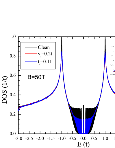
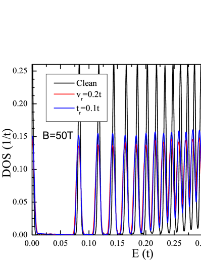
Figure 7: (a) DOS of clean graphene (black lines) and of disordered graphene with a random on-site potential (red lines) and with a random renormalization of the hopping integrals (blue lines). The inset shows the smearing of the VHS peak due to disorder. (b) Zoom of the low energy part of the spectrum.

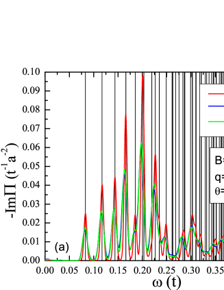
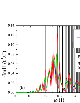
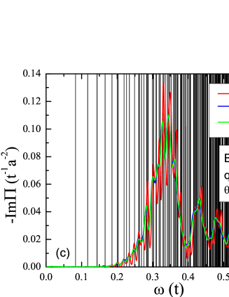
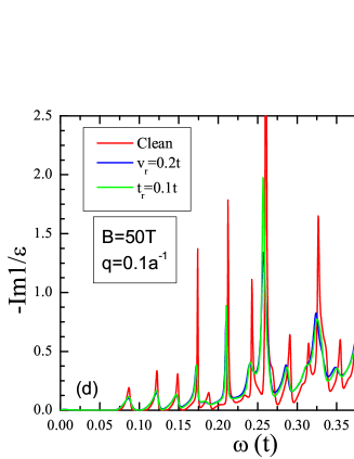
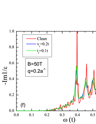
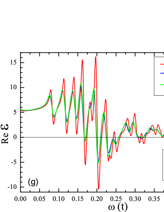
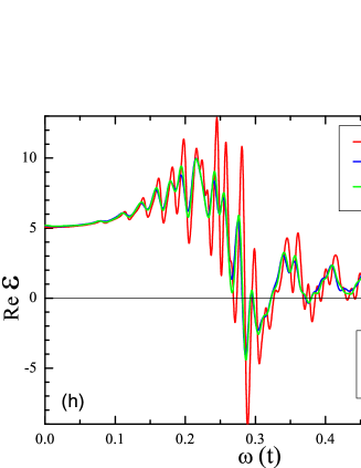
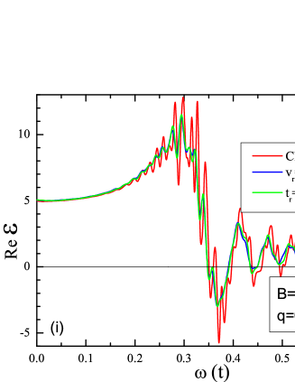
Figure 8: (a)-(c) Non-interacting single-particle excitation spectrum of graphene in a magnetic field of $B=50$T, as defined by $-\mathrm{Im}\Pi(\mathbf{q},\omega)$, for different kinds of disorder and for different values of the wave-vector $q$. The black vertical lines signal the energy of the electron-hole processes defined by Eq. (20). (d)-(f) Loss function $-\mathrm{Im}[1/\varepsilon(\mathbf{q},\omega)]$ in the RPA. (g)-(i) Real part of the dielectric function $\mathrm{Re}~{}\varepsilon(\mathbf{q},\omega)$ in the RPA.

Well defined LLs occur around the Dirac point, and the effect of disorder on the peaks is observed in Fig. 7, where we show a zoom of the low energy part of the DOS around $\epsilon=0$. Both kinds of disorder (random on-site potential and random hopping) leads to a similar effect, producing a broadening of the LLs. We can also observe, especially for the highest LLs shown in Fig. 7(b), a tiny but appreciable redshift of the position of the center of the LLs with respect to its original position, in agreement with previous works.Shon and Ando (1998); Pereira et al. (2011) The full self-consistent Born approximation calculations for graphene with unitary scatterers of Ref. Peres et al., 2006 leaded to a rather significant change in the position of the LLs towards higher energies. However, the exact transfer matrix and diagonalization calculations of Ref. Goswami et al., 2008 found only a small shift of the LL position for very strong disorder.

We now study the effect of disorder on the PHES. In Fig. 8(a)-(c) we show $-\mathrm{Im}\Pi(\mathbf{q},\omega)$ for different values of $q$, and for different kinds of disorder. First we notice a smearing of the resonance peaks associated to the LL broadening due to disorder. Whereas for low energies the position of the resonance peaks of disordered graphene coincides with the position for the clean case, we observe a redshift of the resonance peaks as we consider inter-LL transitions of higher energies. This is due to the change in the position of the high energy LLs of disordered graphene with respect to the original LLs, as we have discussed previously [see Fig. 7(b)].

The presence of disorder will also affect the dispersion relation and coherence of the collective modes when the effect of electron-electron interaction is included. In particular, the effect of a short range disorder on graphene in a magnetic field can lead, due to the possibility of inter-valley processes associated to the breakdown of sublattice symmetry, to the localization of some collective modes on the impurity.Fischer et al. (2011) In Fig. 8(d)-(f) we show the effect of a random on-site potential or a random hopping renormalization on the loss function. First, we can observe an important attenuation of the intensity peaks due to disorder. Second, as we have discussed above, the position of the peaks of disordered and clean graphene coincides at low energies, but not at high energies, where the resonance peaks of the loss function of disordered graphene are shifted with respect to clean graphene. Although we obtain a similar renormalization of the spectrum for the two kinds of disorder considered here, we reiterate that this effect is highly dependent on the type disorder considered, as well as the theoretical method used to obtain the spectrum.

Finally, we mention that the disorder LL broadening leads to an amplification of the LL mixing discussed above. As a consequence, some collective modes which are undamped for clean graphene, start to be Landau damped due to the effect of disorder. Indeed, in Fig. 8(g)-(i) we can see how Eq. (12), which is the condition for the existence of coherent collective modes, is fulfilled more times for the clean case than for the disordered membranes, for which the collective modes are more highly damped.

IV.2 Effect of temperature: thermally activated electron-hole transitions

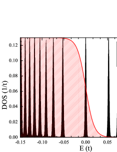
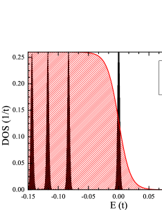
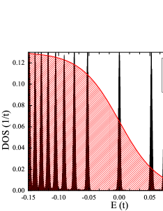
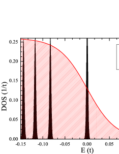
Figure 9: DOS of clean graphene for different values of temperature $T$ and magnetic field $B$. The shaded area is a sketch of the Fermi-Dirac distribution function for each case.

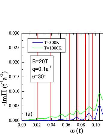
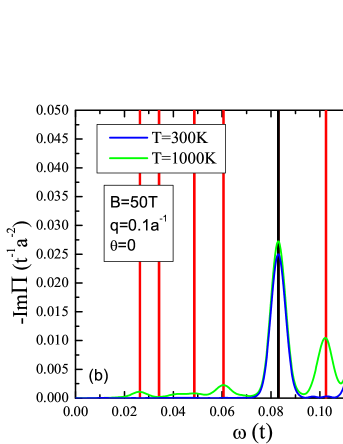
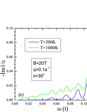
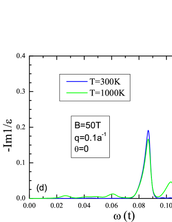
Figure 10: (a)-(b) $-\mathrm{Im}\Pi(\mathbf{q},\omega)$ for two different values of $T$ and $B$. The black vertical lines denote the position of the inter-LL transitions given by Eq. (20) which are possible at $T=0$. The red vertical lines correspond to the energy of thermally activated inter-LL transitions. (c)-(d) Loss function $-\mathrm{Im}[1/\varepsilon(\mathbf{q},\omega)]$ for the same values of $T$ and $B$.

In this subsection we discuss the effect of temperature on the excitation spectrum, which enters in our calculations trough the Fermi-Dirac distribution function Eq. (8). Temperature can activate additional inter-LL transitions due to free thermally induced electrons and holes in the sample. In Fig. 9 we sketch the LLs of undoped clean graphene that are thermally activated, for two different strengths of the magnetic field. For this, the corresponding Fermi-Dirac distribution function is sketched on each plot, indicating the LLs that can be partially populated with electrons (holes) in the conduction (valence) band. Notice that at $T=0$ and for $\mu=0$, $n_{F}(\epsilon)$ is just a step function that traverses the $n=0$ LL. Of course, the number of activated LLs, which are those crossed by the tail of $n_{F}(\epsilon)$, grows as we increase the temperature and/or as we decrease the magnetic field. The population effect due to the thermal excitations of carriers has been observed by far infrared transmission experiments.Orlita et al. (2008)

In Fig. 10 we show the single-particle polarization and the loss function for two values of temperature and magnetic field. At room temperature and for the rather strong magnetic fields considered in our calculation, the allowed electron-hole transitions are the same as in the zero temperature limit (see the top panels of Fig. 9). Therefore, the peaks of $\mathrm{Im}\Pi$ for $T=300$ K are centered at the frequencies of inter-LL transitions marked by the black vertical lines, which accounts only for the usual inter-band transitions across the Dirac point. For a considerable higher temperature of $T=10^{3}$ K there are additional electron-hole transitions (some of them intra-band processes, especially important at low frequencies) which are now allowed due to the effect of temperature, as marked by the red vertical lines in Fig. 10(a)-(b). These thermally activated inter-LL transitions at high temperatures contribute to the additional spectral weight of the PHES of Fig. 10(a)-(b). Finally, in Fig. 10(c)-(d) we show the loss functions corresponding to the magnetic fields and temperatures discussed above. As we have discussed above, the peaks of $\mathrm{Im}~{}1/\varepsilon$ correspond to the position of collective excitations. Here we find, in agreement with previous tight-binding and band-like matrix numerical methods,Wu et al. (2011) a weak but appreciable renormalization of the collective mode peak position as a function of temperature. This temperature dependence of the collective mode is easily noticed by comparing the red and blue peaks at $\omega\approx 0.12t$ of Fig. 10(d).

V Conclusions

In conclusion, we have studied the excitation spectrum of a graphene layer in the presence of a strong magnetic field, using a full $\pi$-band tight-binding model. The magnetic field has been introduced by means of a Peierls substitution, and the effect of long range Coulomb interaction has been considered within the RPA. For realistic values of the magnetic field, the LL quantization leads to well defined LLs around the Dirac point, whereas the DOS at higher energies is rater similar to the one at zero field. However, we have shown that in the ultra-high magnetic field limit,Singha et al. (2011) for which the magnetic length is comparable to the lattice spacing, the LL quantization around the Van Hove singularity is highly nontrivial, with two different sets of LLs that merge at the saddle point.

Our results for the polarization function shows that, at high energies, the PHES is dominated, as in the $B=0$ case,Yuan et al. (2011a) by the $\pi$-plasmon, which is associated to the enhanced DOS at the VHS of the $\pi$ bands. The low energy part of the spectrum is however completely different to its zero field counterpart. The relativistic LL quantization of the spectrum into non-equidistant LLs lead to a peculiar excitation spectrum with a strong modulation of the spectral weight, which can be understood in terms of the node structure of the electron-hole wavefunction overlap.Roldán et al. (2010a) Furthermore, we have shown that the presence of disorder in the sample lead to a smearing of the resonance peaks of the loss function, and to an enhancement of the Landau damping of the collective modes. Finally, we have studied the effect of temperature on the spectrum, and shown that it can activate additional inter-LL transitions, effect which is especially relevant at low magnetic fields.

VI Acknowledgement

The support by the Stichting Fundamenteel Onderzoek der Materie (FOM) and the Netherlands National Computing Facilities foundation (NCF) are acknowledged. We thank the EU-India FP-7 collaboration under MONAMI and the grant CONSOLIDER CSD2007-00010.

References

- Novoselov et al. (2005) K. S. Novoselov, A. K. Geim, S. V. Morozov, D. Jiang, M. I. Katsnelson, I. V. Grigorieva, S. V. Dubonos, and A. A. Firsov, Nature (London) 438, 197 (2005).
- Zhang et al. (2005) Y. Zhang, Y.-W. Tan, H. L. Stormer, and P. Kim, Nature (London) 438, 201 (2005).
- Katsnelson (2012) M. I. Katsnelson, Graphene: Carbon in Two Dimensions (Cambridge, Cambridge Univ. Press, 2012).
- Goerbig (2011) For a recent review on the electronic properties of graphene in a magnetic field, see e.g. M. O. Goerbig, Rev. Mod. Phys. 83, 1193 (2011).
- Shung (1986) K. W. K. Shung, Phys. Rev. B 34, 979 (1986).
- Wunsch et al. (2006) B. Wunsch, T. Stauber, F. Sols, and F. Guinea, New Journal of Physics 8, 318 (2006).
- Hwang and Sarma (2007) E. H. Hwang and S. D. Sarma, Phys. Rev. B 75, 205418 (2007).
- Roldán et al. (2010a) R. Roldán, M. O. Goerbig, and J.-N. Fuchs, Semicond. Sci. Technol. 25, 034005 (2010a).
- Pyatkovskiy and Gusynin (2011) P. K. Pyatkovskiy and V. P. Gusynin, Phys. Rev. B 83, 075422 (2011).
- Iyengar et al. (2007) A. Iyengar, J. Wang, H. A. Fertig, and L. Brey, Phys. Rev. B 75, 125430 (2007).
- Shizuya (2007) K. Shizuya, Phys. Rev. B 75, 245417 (2007).
- Gusynin et al. (2007) V. P. Gusynin, S. G. Sharapov, and J. P. Carbotte, International Journal of Modern Physics B 21, 4611 (2007).
- Bychkov and Martinez (2008) Y. A. Bychkov and G. Martinez, Phys. Rev. B 77, 125417 (2008).
- Roldán et al. (2009) R. Roldán, J.-N. Fuchs, and M. O. Goerbig, Phys. Rev. B 80, 085408 (2009).
- Shizuya (2010) K. Shizuya, Phys. Rev. B 81, 075407 (2010).
- Wu et al. (2011) J.-Y. Wu, S.-C. Chen, O. Roslyak, G. Gumbs, and M.-F. Lin, ACS Nano 5, 1026 (2011).
- Sadowski et al. (2006) M. L. Sadowski, G. Martinez, M. Potemski, C. Berger, and W. A. de Heer, Phys. Rev. Lett. 97, 266405 (2006).
- Jiang et al. (2007) Z. Jiang, E. A. Henriksen, L. C. Tung, Y.-J. Wang, M. E. Schwartz, M. Y. Han, P. Kim, and H. L. Stormer, Phys. Rev. Lett. 98, 197403 (2007).
- Deacon et al. (2007) R. S. Deacon, K.-C. Chuang, R. J. Nicholas, K. S. Novoselov, and A. K. Geim, Phys. Rev. B 76, 081406 (2007).
- Henriksen et al. (2010) E. A. Henriksen, P. Cadden-Zimansky, Z. Jiang, Z. Q. Li, L.-C. Tung, M. E. Schwartz, M. Takita, Y.-J. Wang, P. Kim, and H. L. Stormer, Phys. Rev. Lett. 104, 067404 (2010).
- Faugeras et al. (2011) C. Faugeras, M. Amado, P. Kossacki, M. Orlita, M. Kühne, A. A. L. Nicolet, Y. I. Latyshev, and M. Potemski, Phys. Rev. Lett. 107, 036807 (2011).
- Plochocka et al. (2008) P. Plochocka, C. Faugeras, M. Orlita, M. L. Sadowski, G. Martinez, M. Potemski, M. O. Goerbig, J.-N. Fuchs, C. Berger, and W. A. de Heer, Phys. Rev. Lett. 100, 087401 (2008).
- Singha et al. (2011) A. Singha, M. Gibertini, B. Karmakar, S. Yuan, M. Polini, G. Vignale, M. I. Katsnelson, A. Pinczuk, L. N. Pfeiffer, K. W. West, and V. Pellegrini, Science 332, 1176 (2011).
- McChesney et al. (2010) J. L. McChesney, A. Bostwick, T. Ohta, T. Seyller, K. Horn, J. González, and E. Rotenberg, Phys. Rev. Lett. 104, 136803 (2010).
- Efetov and Kim (2010) D. K. Efetov and P. Kim, Phys. Rev. Lett. 105, 256805 (2010).
- Luttinger (1951) J. M. Luttinger, Phys. Rev. 84, 814 (1951).
- Castro Neto et al. (2009) A. H. Castro Neto, F. Guinea, N. M. R. Peres, K. Novoselov, and A. K. Geim, Rev. Mod. Phys. 81, 109 (2009).
- Hams and De Raedt (2000) A. Hams and H. De Raedt, Phys. Rev. E 62, 4365 (2000).
- Yuan et al. (2010) S. Yuan, H. De Raedt, and M. I. Katsnelson, Phys. Rev. B 82, 115448 (2010).
- Kubo (1957) R. Kubo, J. Phys. Soc. Jpn. 12, 570 (1957).
- Yuan et al. (2011a) S. Yuan, R. Roldán, and M. I. Katsnelson, Phys. Rev. B 84, 035439 (2011a).
- Shoenberg (1984) D. Shoenberg, Magnetic Oscillations in Metals (Cambridge, Cambridge Univ. Press, 1984).
- Fuchs et al. (2010) J. N. Fuchs, F. Piéchon, M. O. Goerbig, and G. Montambaux, Eur. Phys. J. B 77, 351 (2010).
- Yuan et al. (2011b) S. Yuan, R. Roldán, and M. I. Katsnelson, Phys. Rev. B 84, 125455 (2011b).
- González et al. (1994) J. González, F. Guinea, and M. A. H. Vozmediano, Nucl. Phys. B 424, 595 (1994).
- Stauber et al. (2010) T. Stauber, J. Schliemann, and N. M. R. Peres, Phys. Rev. B 81, 085409 (2010).
- Eberlein et al. (2008) T. Eberlein, U. Bangert, R. R. Nair, R. Jones, M. Gass, A. L. Bleloch, K. S. Novoselov, A. Geim, and P. R. Briddon, Phys. Rev. B 77, 233406 (2008).
- Roldán et al. (2010b) R. Roldán, J.-N. Fuchs, and M. O. Goerbig, Phys. Rev. B 82, 205418 (2010b).
- Lozovik and Sokolik (2011) Y. E. Lozovik and A. A. Sokolik, ArXiv e-prints (2011), arXiv:1111.1176 .
- Kallin and Halperin (1984) C. Kallin and B. I. Halperin, Phys. Rev. B 30, 5655 (1984).
- Pereira (2009) A. L. C. Pereira, New Journal of Physics 11, 095019 (2009).
- Pereira et al. (2011) A. L. C. Pereira, C. H. Lewenkopf, and E. R. Mucciolo, Phys. Rev. B 84, 165406 (2011).
- Shon and Ando (1998) N. H. Shon and T. Ando, J. Phys. Soc. Jpn. 67, 2421 (1998).
- Peres et al. (2006) N. M. R. Peres, F. Guinea, and A. H. Castro Neto, Phys. Rev. B 73, 125411 (2006).
- Goswami et al. (2008) P. Goswami, X. Jia, and S. Chakravarty, Phys. Rev. B 78, 245406 (2008).
- Fischer et al. (2011) A. M. Fischer, R. A. Römer, and A. B. Dzyubenko, Phys. Rev. B 84, 165431 (2011).
- Orlita et al. (2008) M. Orlita, C. Faugeras, P. Plochocka, P. Neugebauer, G. Martinez, D. K. Maude, A.-L. Barra, M. Sprinkle, C. Berger, W. A. de Heer, and M. Potemski, Phys. Rev. Lett. 101, 267601 (2008).