Variability Selected Low-Luminosity Active Galactic Nuclei in the 4 Ms Chandra Deep Field-South
Abstract
The 4 Ms Chandra Deep Field-South (CDF-S) and other deep X-ray surveys have been highly effective at selecting active galactic nuclei (AGN). However, cosmologically distant low-luminosity AGN (LLAGN) have remained a challenge to identify due to significant contribution from the host galaxy. We identify long-term X-ray variability (month–years, observed frame) in 20 of 92 CDF-S galaxies spanning redshifts that do not meet other AGN selection criteria. We show that the observed variability cannot be explained by X-ray binary populations or ultraluminous X-ray sources, so the variability is most likely caused by accretion onto a supermassive black hole. The variable galaxies are not heavily obscured in general, with a stacked effective power-law photon index of , and are therefore likely LLAGN. The LLAGN tend to lie a factor of 6–80 below the extrapolated linear variability-luminosity relation measured for luminous AGN. This may be explained by their lower accretion rates. Variability-independent black-hole mass and accretion-rate estimates for variable galaxies show that they sample a significantly different black-hole mass-accretion rate space, with masses a factor of 2.4 lower and accretion rates a factor of 22.5 lower than variable luminous AGN at the same redshift. We find that an empirical model based on a universal broken power-law PSD function, where the break frequency depends on SMBH mass and accretion rate, roughly reproduces the shape, but not the normalization, of the variability-luminosity trends measured for variable galaxies and more luminous AGN.
Subject headings:
galaxies: active — X-rays: galaxies1. Introduction
Observations show that all nearby galaxies with a massive bulge component host supermassive black holes (SMBHs) (e.g., Ferrarese & Ford, 2005; Gültekin et al., 2009). SMBHs accreting near the Eddington limit (/ 0.1–1) are visible as luminous active galactic nuclei (AGN) that often outshine their host galaxies. Models of AGN lifetime, constrained by observed Eddington ratio distributions, suggest that SMBH growth is dominated by this luminous phase, lasting a few 108 years (e.g., Marconi et al., 2004; Shankar et al., 2004; Hopkins & Hernquist, 2009).
Observations including constraints on the sizes of ionized “bubbles” around quasars (e.g., Jakobsen et al., 2003; Goncalves et al., 2008) and the lengths of relativistic jets and radio lobes (e.g., Scheuer, 1995; Blundell et al., 1999) suggest that the episodic lifetime of luminous activity is similar to the total lifetime, implying that a SMBH is triggered to the luminous AGN phase no more than a few times. SMBHs therefore spend significant amounts of time in quiescent or low-activity phases, which may contribute up to 20% of overall SMBH growth (Hopkins & Hernquist, 2009). A SMBH accreting at lower rates (/ 0.1) will appear as a low-luminosity AGN (LLAGN). LLAGN share several properties with more luminous AGN, including similar X-ray spectral shapes (e.g., Younes et al., 2011) and similar radio-loud fractions and luminosity-dependent, intrinsic X-ray to optical flux ratios (e.g., Maoz, 2007). A more complete census of LLAGN is important for understanding SMBH accretion history, but the relative significance of the host galaxy in LLAGN makes a full census of accretion activity a challenge.
Deep X-ray surveys have been effective at selecting a wide variety of AGN, including luminous, unobscured AGN as well as faint and/or obscured AGN (e.g., see Brandt & Hasinger, 2005, for a review). X-ray selection criteria usually include cuts on X-ray luminosity and X-ray spectral shape. Multi-wavelength data further aid X-ray selection by allowing selection via, for example, excess X-ray emission compared to what is expected from optical flux (e.g., Hornschemeier et al., 2003) or radio luminosity (e.g., Alexander et al., 2005).
The above methods have been successful in selecting a wide variety of AGN, but nevertheless miss certain populations, such as very heavily obscured AGN and LLAGN (e.g., Bauer et al., 2004; Alexander et al., 2005; Lehmer et al., 2008). While heavily obscured AGN can often be selected in the IR (e.g., Houck et al., 2005; Martinez-Sansigre et al., 2005; Alexander et al., 2008), the spectral energy distributions (SEDs) of LLAGN are likely dominated by the host galaxy in other bands. Even in X-rays, X-ray binaries, ultraluminous X-ray sources, and hot gas will provide significant contributions to the overall power output. Simulated Chandra observations of nearby low-luminosity Seyfert nuclei artificially shifted to show that LLAGN would exhibit X-ray luminosities, spectral shapes, and X-ray-to-optical flux ratios consistent with those of normal or optically bright/X-ray faint galaxies (Peterson et al., 2006). By relying on such criteria, deep X-ray surveys may be underestimating AGN fractions.
Variability potentially provides a useful indicator of whether an extragalactic X-ray source, classified as a galaxy by other means, harbors an AGN. Variability is a defining characteristic of AGN and has long been used as an AGN selection technique (e.g., van den Bergh et al., 1973). Numerous studies have used optical variability to select AGN from deep surveys such as the 1 Ms CDF-S, the Subaru/XMM-Newton Deep Field, and the GOODS North and South Fields (e.g., Trevese et al., 2008; Morokuma, 2008; Villforth et al., 2010; Sarajedini et al., 2011, respectively). Spectroscopic observations of the 1 Ms CDF-S (Boutsia et al., 2009) found that 17 of 27 optical variability-selected objects were broad-line AGN; 9 (5) AGN would have been missed if selected by color (X-ray selection).
Similarly, UV variability has been used successfully to identify LLAGN in galaxies with low-ionization nuclear emission-line regions (LINERs). LINERs have been found in the nuclei of a large fraction of nearby galaxies (e.g., Ho et al., 1997; Kauffman et al., 2003), but these regions could be ionized by either massive star clusters or low accretion-rate AGN. HST imaging has found that 25% of LINERs are associated with compact ( few pc) UV sources (Maoz et al., 1995; Barth et al., 1998). A study of LINERs with compact nuclear UV sources found significant variability in 15 of 17, indicating the presence of an AGN (Maoz et al., 2005).
Deep X-ray surveys are able to detect variability in moderate-luminosity/high-redshift AGN (e.g., Almaini et al., 2000; Paolillo et al., 2004; Papadakis et al., 2008b). The 4 Ms Chandra Deep Field-South (Xue et al., 2011), the deepest X-ray survey to date, allows a preliminary classification of AGN on the basis of several observed quantities (see §2 for details). This paper utilizes X-ray variability techniques to search for AGN missed by these criteria. With 4 Ms of exposure time spanning 10.8 years for 466 good-quality sources (see §3), variability can be detected in sources with time-averaged fluxes as faint as ergs cm-2 s-1. We use a cosmology with H0 = 70.4 km s-1 Mpc-1, = 0.272, and = 0.728 (e.g., Komatsu et al., 2011).
2. Overview of the 4 Ms CDF-S Catalog
The details of the 4 Ms CDF-S source catalog are available in Xue et al. (2011); we provide a brief summary here. The 4 Ms CDF-S, constructed from 54 Chandra observations over 10.8 years, covers an area of 464.5 arcmin2 and reaches highest sensitivities of ergs cm-2 s-1 and ergs cm-2 s-1, with multi-wavelength coverage in more than 40 bands from the radio to the UV. Source candidates are detected using a 10-5 false-positive probability threshold in wavdetect (Freeman et al., 2002) and are then pruned using a binomial no-source probability (see Appendix A2 of Weisskopf et al. 2007) 0.004 to obtain a more conservative list of 740 main-catalog sources, all of which are consistent with being point sources. Source extraction and photometry were conducted with acis extract (AE; Broos et al. 2010). AE models Chandra’s High Resolution Mirror Assembly point spread function (PSF) using the MARX ray-tracing simulator.111MARX is available at http://space.mit.edu/CXC/MARX/index.html The PSF model is used to generate a polygonal extraction region for each source that approximates the 90% encircled energy fraction (EEF) contour of a local PSF measured at 1.497 keV. For 6% of the candidates, the sources are crowded (i.e., the polygonal source regions overlap) and smaller extraction regions that are as large as possible without overlapping (% EEF) are used. The background is calculated from regions that subtract the contribution from the source of interest and its neighboring sources; the regions are typically a factor 16 larger than the source-extraction region. AE merges the individual observations to estimate aperture-corrected, background-subtracted counts and the 1 (asymmmetric) upper and lower statistical errors (Gehrels, 1986). In this paper, we will use the standard X-ray photometric bands: 0.5–2 keV (soft), 2–8 keV (hard), and 0.5–8 keV (full).
Though most sources have a relatively small number of counts (median net counts 77), a rough estimate of source spectral shape can be made by relating the band ratio (i.e., the ratio of the count rates in the 2–8 keV and 0.5–2 keV bands) to an effective power-law photon index, ( ). For low-count sources where cannot be determined reliably, is set to 1.4, the stacked (co-added) spectrum of all sources in the CDF-S (Tozzi et al., 2001; Xue et al., 2011), which is consistent with the unresolved spectrum of the cosmic X-ray background (Hickox & Markevitch, 2006).
Of 740 X-ray sources, 716 (96.8%) contain matches in at least one of seven optical/near-infrared/radio (ONIR) catalogs: (1) the ESO 2.2 m WFI -band catalog (Giavalisco et al., 2004), (2) the GOODS-S Hubble Space Telescope () version r2.0z -band catalog (Giavalisco et al., 2004), (3) the GEMS HST -band catalog (Caldwell et al., 2008), (4) the GOODS-S MUSIC catalog (Grazian et al., 2006), (5) the MUSYC -band catalog (Taylor et al., 2009), (6) the SIMPLE Spitzer/IRAC 3.6m catalog (Damen et al., 2011), and (7) the VLA 1.4 GHz radio catalog (Miller et al., 2008).
Of 716 X-ray sources with multi-wavelength identifications, 419 (58.5%) have spectroscopic redshift measurements, collected from Le Fèvre et al. (2004), Szokoly et al. (2004), Zheng et al. (2004), Mignoli et al. (2005), Ravikumar et al. (2007), Vanzella et al. (2008), Popesso et al. (2009), Treister et al. (2009), Balestra et al. (2010), and Silverman et al. (2010). A total of 343 (81.9%) of the 419 spectroscopic redshift measurements are “secure”, in that they are measured at 95% confidence levels with multiple secure spectral features. 668 (93.3%) sources have high-quality, accurate (/() 6.5%) photometric-redshift measurements from at least one of three photometric-redshift catalogs: Cardamone et al. (2010), Luo et al. (2010), and Rafferty et al. (2011). The positions of primary ONIR counterparts were cross-matched with the photometric-redshift catalogs using a matching radius of 0.5′′, resulting in a false-match probability of 1%. Subsequent spectroscopic observations published in the Arizona CDF-S Environment Survey (ACES; Cooper et al. 2012) catalog show with a blind test that errors on the photometric redshifts are 1%.
The 4 Ms CDF-S X-ray sources were classified as AGN by the following criteria:
High luminosities: ergs s-1, where the rest-frame luminosity has been corrected for Galactic and intrinsic absorption.
Hard spectra: A source with 1.0 is identified as a heavily obscured AGN.
High X-ray-to-optical flux ratios: log(/) , where = , , or and is the -band flux.
Excess X-ray emission compared to that expected from star formation: ( ) (Alexander et al., 2005), where is the 1.4 GHz monochromatic luminosity in W Hz-1.
An indication of broad emission lines in the optical spectrum.
Stars were classified by cross-matching X-ray sources (using the ONIR counterpart positions) with (1) the spectroscopically identified stars in Szokoly et al. (2004), Mignoli et al. (2005), and Silverman et al. (2010); (2) the likely stars with stellarity indices greater than 0.7 in the GEMS HST catalog (Caldwell et al., 2008); and (3) the likely stars with best-fit stellar templates in the MUSYC photometric-redshift catalog (Cardamone et al., 2010), using a matching radius of 0.5′′.
X-ray sources not identified as an AGN or a star were classified as galaxies.
Rest-frame 0.5–8 keV luminosities are calculated for all sources. For AGN, which make up the vast majority of CDF-S sources, the luminosity is corrected for Galactic and intrinsic absorption. AGN not detected in the full band have an upper limit on the X-ray luminosity based on the 3 Poisson error on the counts. For galaxies, the intrinsic-absorption correction and -corrections may not be appropriate. Of 92 CDF-S galaxies with “good quality” observations (see §3), 78 are not detected in the hard band and have poorly determined photon indices. All galaxies are detected in the soft-band. We perform a stacking analysis for galaxies with 150 net counts (87 of 92) following the procedure described in §5.1. The resulting average = 1.900.08 gives / = 2.35. We calculate the rest-frame 0.5–8 keV luminosity for CDF-S galaxies as . Since galaxy X-ray emission is typically unabsorbed, we do not apply any correction for intrinsic absorption.
3. Testing for X-ray Variability
We perform two quality cuts before conducting variability analysis. First, we exclude the catalog sources with off-axis angles greater than 8′ to ensure that sources will have sufficient coverage (50 of 54 observations) throughout the various CDF-S pointings. To ensure accurate variability measurements, we also require that each source has at least 20 net counts in the 0.5–8.0 keV band (i.e., at least 5 counts on average per epoch, as defined below). These quality cuts result in a total sample of 466 CDF-S sources: 369 classified as AGN, 92 classified as galaxies, and 5 classified as stars in the Xue et al. (2011) catalog. All of these AGN and galaxies have measured spectroscopic or photometric redshifts. The 92 sources classified as galaxies may nevertheless contain an AGN, as would be indicated by X-ray variability, and make up the sample investigated in this paper.
We divide the CDF-S observations into four epochs, each containing 1 Ms of integration: 2000 (943.1 ks), 2007 (967.7 ks), 2010a (March–May; 1015.5 ks), and 2010b (May–July; 944.9 ks). As in Xue et al. (2011), we merged observations within each epoch and, for a given source position from the CDF-S catalog, measured the source and background counts and flux over three observed-frame energy bands: 0.5–8 keV, 0.5–2 keV, and 2–8 keV. A source is considered variable if the variability observed between observations is greater than that expected from Poisson statistics, with a probability threshold of 5% that the variability is due to noise alone. (The choice of probability threshold is discussed further below.) To check whether a source can be considered variable, we calculate the quantity:
| (1) |
where is the number of epochs, is the photon flux (background-subtracted counts with units of cm-2 s-1) in a given epoch, is the mean photon flux over all epochs, and is the error squared on the photon flux for the epoch. The photon flux is calculated by dividing the full-band (0.5–8.0 keV) net counts by the exposure time and the mean effective area across the source aperture. The Gehrels (1986) approximation gives the error on the net counts, which is propagated to obtain the error on the photon flux. Since this error is significantly asymmetric for low-count ( counts) sources, we average the upward and downward error bars for these objects to obtain the average error . (The same method is applied in the Monte Carlo simulations below.)
For large photon fluxes, the statistic follows a distribution, and any source with 7.82 (for 3 degrees of freedom) has a probability 0.05 (i.e., 95% confidence level) that the variability is due to random noise. However, at low count rates, the error on the photon flux is not Gaussian. Since errors in the low-count regime are larger than expected from a Gaussian distribution, the resulting statistic is smaller than expected and does not follow the distribution (see Fig. 2 of Paolillo et al. 2004).
We therefore constructed a Monte Carlo simulation to determine the distribution the statistic should follow for each source, similar to the procedure followed by Paolillo et al. (2004). We first scaled the total observed source and background counts for each source, obtained from the full 4 Ms observation, to the exposure time and effective area for a given epoch. This procedure generates the source and background counts expected in each epoch if the source and background were constant over time, and it accounts for fluctuations in the background that will affect low-count sources. To simulate the variance expected from noise, Poisson distributions were defined using the expected source and background counts as the mean values. We then simulated 1,000 observations of each source by repeatedly drawing the expected counts from the Poisson distributions. For each simulated observation, we calculated the photon flux for four epochs and calculated as defined above. Asymmetric errors on the source and background counts are obtained from Gehrels (1986) and are propagated to get the error on the photon flux. The observed can then be compared to the simulated distribution to determine the probability that the observed variability is due to Poisson noise. Spurious sources of variability are negligible, since effective exposure maps are calculated separately for each observation, taking into account issues such as vignetting, CCD gaps, bad pixels, bad columns, and Chandra’s spatial- and time-dependent quantum efficiency degradation.
While using a more conservative = 1% on our dataset would result in fewer false positives, it would also eliminate a similar number of truly varying sources. For example, in the sample of 92 galaxies, = 5% results in 20 variable sources (see §4), of which 4.6 are expected to be false positives. Reducing to 1% results in 13 variable sources, of which 0.9 is expected to be a false positive. So while the more conservative critical value eliminates 4 false positives, it also eliminates truly varying sources. The values listed in Table 2 can be used to screen the sources further as desired.
4. Galaxies with AGN-like Variability
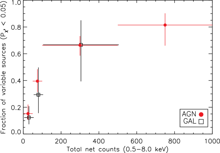
Of the 369 CDF-S sources classified as AGN that meet both the off-axis angle ( 8′) and count (total net counts 20) requirements, 50.1% exhibit significant flux variability ( 0.05) on month–year timescales. For the 178 AGN with more than 100 counts, 74.2% exhibit significant variability. The basic diagnostic plot in Figure 1 shows the rise in the AGN variable fraction with total net counts. The plot demonstrates that, given sufficient counts to detect it, variability is a near-ubiquitous property of faint, X-ray selected AGN, even in the case of significant obscuration: 70% of the CDF-S sample consists of obscured AGN (Xue et al., 2011), and 47.5% (51.5%) of obscured (unobscured) AGN are significantly variable. The variable fractions are consistent with the results from the 1 Ms CDF-S (Paolillo et al., 2004), although obtained with different temporal sampling and down to much fainter fluxes.
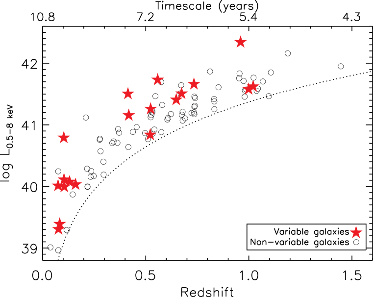
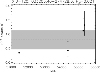
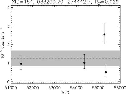
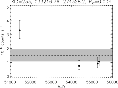
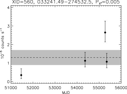
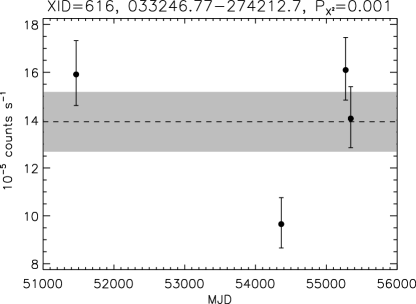
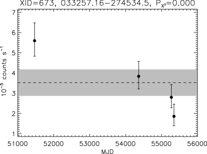
In sources classified as galaxies, the variable fraction is significant at low counts and equals that of AGN at higher counts (Figure 1). Table 1 describes the columns of Table 2, which lists the attributes of the 20 variable and 72 non-variable galaxies. (Variability properties of CDF-S AGN will be covered in the forthcoming Paolillo et al., in preparation.) The luminosity-redshift distribution of variable and non-variable galaxies is shown in Figure 2; almost all lie below . Spectroscopic redshifts are available for 18 of 20 variable galaxies and for 61 of 72 non-variable galaxies. Photometric redshifts are available for the remaining sources. Six example light curves (background-subtracted count rates in the observed-frame 0.5-8 keV band vs. MJD) representative of the sample as a whole are shown in Figure 3.
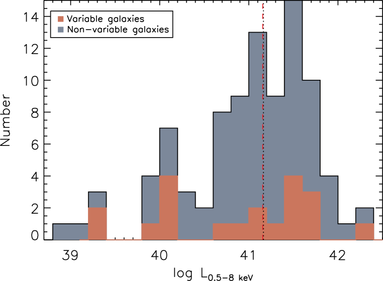
The X-ray luminosity distributions of all CDF-S galaxies and those exhibiting significant variability are shown in Figure 4. A K-S test shows that the two samples are consistent with being drawn from the same parent population ( = 57%), and the variable fraction does not show a significant dependence on X-ray luminosity below 1043 ergs s-1. The possibility that AGN-related variability may go undetected in galaxies is discussed in §4.1.
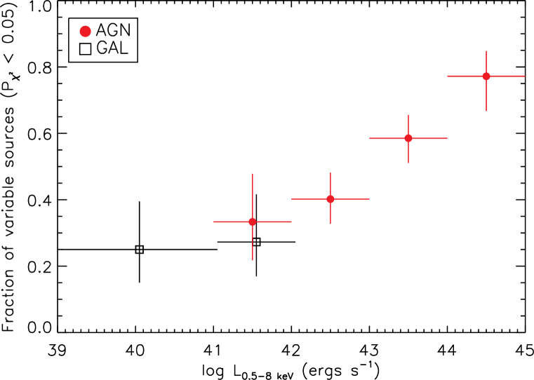
We briefly compare AGN selection based on variability to the following selection methods: (1) X-ray luminosity cuts, (2) the X-ray-to-optical flux ratio, and (3) excess X-ray emission compared to that expected from star formation, based on the radio luminosity. Figure 5 shows the fraction of variable sources vs. X-ray luminosity. Below = 1042 ergs s-1, a luminosity cut often used for AGN selection in X-ray surveys, the variable fraction remains significant at . Of 64 CDF-S galaxies with 1042 ergs s-1, 17 (27%) are variable.
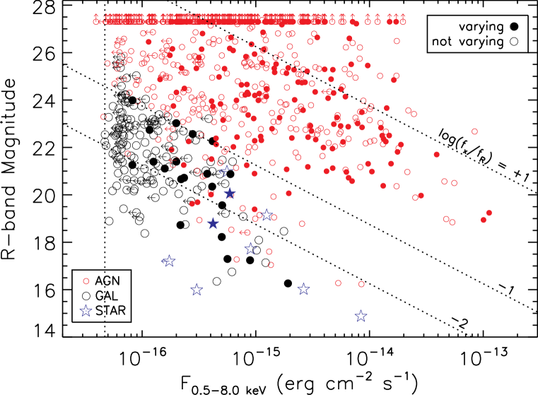
AGN selection via the X-ray-to-optical flux ratio is demonstrated by the -band magnitude vs. X-ray flux plane in Figure 6 (cf. Figure 16 in Xue et al. 2011). Sources classified as AGN, galaxies, and stars in Xue et al. (2011) are marked as small red circles, larger black circles and blue stars, respectively. Variable sources are marked with filled symbols. The optically bright, X-ray faint region, typically thought to exclude AGN (OBXF; /; Hornschemeier et al. 2003) contains 27 galaxies. Of these, 6 (22%) are variable, with X-ray luminosities spanning log 39.7–41.4.
AGN may also be selected based on a comparison between X-ray and radio luminosities (Xue et al., 2011). The radio luminosity can be used to predict the X-ray luminosity in star-forming galaxies (e.g., Alexander et al., 2005, and references therein), so sources with excess X-ray emission may be classified as AGN. Of the 17 CDF-S galaxies with radio detections (none of which have excess X-ray emission), three (18%) are variable. These objects may have excess radio emission due to strong radio cores rather than star formation.
4.1. Measuring Variability Strength
Due to the generally limited photon statistics of the CDF-S galaxy sample, most variable sources must be strongly variable to be detected. Significantly variable galaxies show maximum-to-minimum flux ratios 1.5–9.3 (median = 4.1) over the observed 10.8-year time frame. The smallest max-to-min ratio (1.5) was measured for 033246.77274212.7 (XID = 616), a source with 500 counts. For most galaxies, total net counts are too low () to detect variability below a factor of 2–3.
To address whether the variable galaxy max-to-min ratios sample the average AGN population or only the highly variable “tip of the iceberg,” we ran a Monte Carlo simulation. The procedure assumed that the entire galaxy population is significantly variable and simulated the variability expected over 10.8 years of observation. Following the procedure in Vaughan et al. (2003), we used the Timmer & Koenig (1995) algorithm to simulate 5,000 light curves based on the mean and variance of the flux for each of the 92 CDF-S galaxies. For non-variable galaxies, the measured variance represents noise in the measured light curve, which gives an upper limit to the variability that could be present. The algorithm produces a random, continuously sampled light curve from a given power spectral density (PSD) function, which we assumed to be described by a broken power-law, where the break frequency depends on SMBH mass and accretion rate (McHardy et al., 2006). Since the break frequency lies outside the range of timescales sampled for most variable galaxies (see §6.3), we simplify the model to a power-law (() ) with index , as is typical for the low-frequency (long-timescale) PSDs for nearby Seyferts (e.g., Vaughan et al., 2003). The time units of the light curves are determined by the minimum and maximum timescales input into the simulation; the light curve durations are adjusted according to each source’s redshift.
We resampled/rebinned the light curve using the CDF-S observing pattern and add Poisson noise to the simulated light curve to account for measurement error. The full simulated light curves was made five times longer than the sampled region in order to produce variation on timescales much longer than those sampled by the data. This reproduces the effect that very long-timescale (low-frequency) variations have on variability measured over shorter timescales (i.e., “red noise leak”).
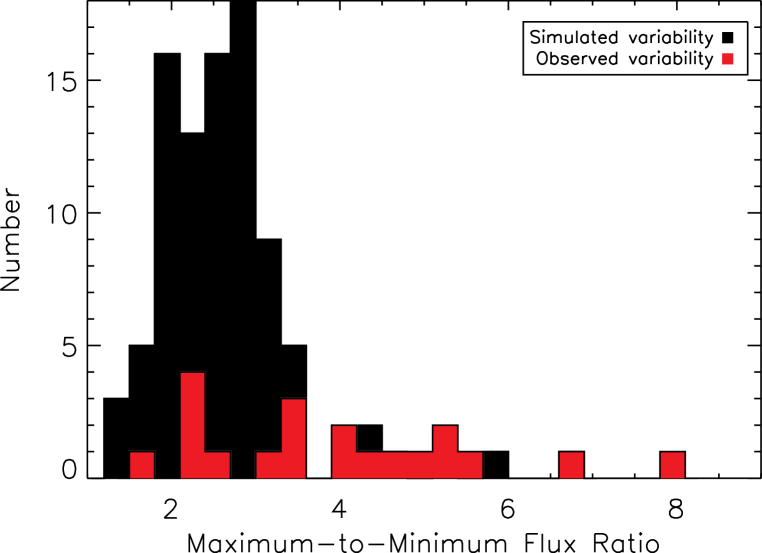
We compare the simulated distribution of median max-to-min ratios, where the median is calculated over 5,000 trials for each galaxy, to the observed distribution for variable galaxies in Figure 7. A K-S test shows that these two populations have a 0.2% chance of being drawn from the same parent population. Note that the simulated distribution (black histogram) illustrates an upper limit to the variability that could be present in the CDF-S, resulting in a lower limit on the detectable fraction of sources. The CDF-S detects at least 18% of sources with max-to-min ratios 2 and at least 57% of sources with max-to-min ratios 4. A significant fraction of non-variable galaxies may still host an AGN, but the variability may remain undetected due to low counts.
For the galaxies exhibiting significant variability, we calculated the normalized excess variance (e.g., Vaughan et al., 2003), which measures how strongly a source varies in excess of the measurement error. The excess variance is the integral of a source’s PSD function over a given frequency range, which is defined by the light curve’s duration (10.8 years, observed-frame) and minimum bin size (4.0 Ms,222While each CDF-S epoch totals 1 Ms in integration time, the timescale sampled is significantly longer due to the spread in Chandra observations, of which the shortest is 4.0 Ms for the 2007 epoch (Luo et al., 2008). observed-frame).
| (2) |
where is the average of the asymmetric upward and downward measurement errors. Using the upward (downward) error would overestimate (underestimate) the errors. Zero excess variance () would indicate that the observed count fluctuation is entirely consistent with noise rather than due to intrinsic source variability; due to statistical fluctuations, the excess variance may also be negative in this case. The values are listed in Table 2. Note that the variability amplitude is calculated for observed-frame energy bands. The variable galaxies cover a redshift range , so the excess variance will be measured over keV at = 0 to keV at = 1. Variability strength is known to depend on energy in some nearby Seyfert galaxies (e.g., Ark 120, MCG–6-30-15, and I Zw 1; Vaughan et al. 2004, Vaughan & Fabian 2004, and Gallo et al. 2007, respectively), while in others, variability remains nearly constant with energy (e.g., Ton S180 and NAB 0205+024; Vaughan et al. 2002 and Gallo et al. 2004, respectively). In the former cases, the change in variability strength is small, with a 10% difference from 0.5 to 10 keV, so the bandpass effects at redshifts should remain small.
We calculate the statistical error (i.e., measurement error) on the excess variance following Equation 11 of Vaughan et al. (2003).
| (3) |
The large errors on (Table 2) are due to the small numbers of counts observed for most sources (e.g., 12 of 20 variable galaxies have 100 net counts); four variable galaxies with net counts 50 have excess variance measurements completely dominated by statistical uncertainty [ err()]. Nevertheless, most variable galaxies have excess variance measured at the 1 level.
The excess variance contains additional sources of uncertainty aside from statistical error: (1) random scatter intrinsic to the stochastic nature of AGN variability (Vaughan et al., 2003) and (2) uncertainty and systematic bias due to sparse sampling of the light curve. The sparse pattern of CDF-S observations will lead to large uncertainty in the mean flux measurement, and since the measured mean will be closer to the sampled data points rather than the true mean, the variance measurements will tend to be underestimated (Allevato et al., in preparation, ). We again employ a Monte Carlo simulation to model the uncertainty and systematic effects produced by random scatter and sparse sampling.
We follow the same procedure described above to produce 5,000 light curves for every variable source. The mean and variance are calculated after sampling each simulated light curve with the CDF-S observing pattern. The sampling bias can be corrected by rescaling the observed variance by a factor equal to the ratio between the “true” input variance (i.e., the observed variance used as input in the simulations) and the median output variance (i.e., the biased variance affected by sparse sampling): = /median(). The median output variance is calculated over all 5,000 light curves. The amount of systematic bias depends on the frequency and regularity of the sampling. If the sampling is regular, the scaling factor will approach unity as the number of samples increases; however, the scaling factor will remain above unity even at high sampling frequency if the sampling is irregular (Allevato et al., in preparation, ). The slope of the PSD will also affect the sampling bias — a steeper PSD slope (i.e., instead of ) will result in a larger bias for a given sampling pattern. Since the intrinsic PSD slopes are not known, we apply uniform corrections assuming ; however, source-to-source variations in PSD slope may be a significant source of scatter in variability measurements.
We find that the scaling factors range from 0.03 to 4.8, with a mean 1.54 and a scatter on of . In 76% of the sources, the scaling factor is greater than unity, indicating that the variance is underestimated due to the sampling bias. Note that the Monte Carlo PSD is normalized by each source’s variance, which is calculated using the source’s light curve. Since the heavy binning could smear out high frequency variations, this method could result in an artificially smaller scaling factor. However, Allevato et al., in preparation, find a similarly small bias () when sampling higher frequencies for a wide range of S/N ratios, gap lengths and sampling patterns. More importantly, the scatter on the factor calculated for each source is large (), so individual measurements, even when corrected for bias, are likely to be poor estimates of the intrinsic variance. Therefore, variability properties of CDF-S galaxies are best considered in ensemble rather than on an individual basis. Bias-corrected excess variances () are listed in Table 2 and are used for all further analysis unless otherwise noted.
4.2. Comparisons with XRB and ULX Variability
The three most likely sources of X-ray variability are X-ray binary (XRB) populations, ultraluminous X-ray sources (ULXs), and accreting SMBHs. In this section, we show that the first two possibilities are not likely to dominate the measured galaxy variability.
To examine the potential contribution of X-ray binary populations to variability, we must first determine the relative contributions of low-mass X-ray binaries (LMXB) and high-mass X-ray binaries (HMXB) to the hard (2–10 keV), galaxy-wide X-ray luminosity ().333We measure variability in the 0.5–8 keV band, but by limiting the comparison to the 2–10 keV luminosities, we limit the contribution of other sources of galaxy-wide X-ray emission (hot gas, supernovae, supernova remnants, and O-stars), which fade sharply above 2 keV and can be considered negligible. Galaxy stellar mass () scales the contribution of (older) LMXBs, and star formation rate (SFR) scales the contribution of (younger) HMXBs (e.g., Equation 3 of Lehmer et al., 2010). and SFR are calculated for each galaxy in Xue et al. (2010) using the optical colors and the UV and IR luminosities. Both the Lehmer et al. (2010) relations and the Xue et al. (2010) calculations adopt the same initial stellar mass function (Kroupa, 2001). However, since Lehmer et al. (2010) and Xue et al. (2010) use different formalisms for computing stellar masses (Bell et al. 2003 and Zibetti et al. 2009, respectively, which differ primarily due to their models of star formation history), we apply a correction factor of 2.6 to the stellar masses from Xue et al. (2010). The SFR and values for each variable galaxy are listed in Table 2.
By comparing the expected LMXB and HMXB contributions to the total luminosity, we can determine which population ought to dominate the variability. In the variable galaxies, SFR ranges from 0.04 to 55 yr-1 with a median of 2.2 yr-1; ranges from to with a median of . We find that all but six of 20 variable galaxies are expected to have a larger HMXB contribution. (SFR)/() ranges from 0.01 to 75.8 with a median of 2.6 (Table 2). HMXBs are generally more variable than LMXBs (Gilfanov et al., 2004), so unless LMXBs dominate the X-ray output of a galaxy, we neglect their contribution.
To determine the variability expected from the HMXBs, we follow the relations in §4.2.3 of Gilfanov et al. (2004), where the variability of the HMXB population is roughly determined by the galaxy’s SFR. The following relations were obtained from Monte Carlo simulations with a power-law HMXB luminosity function with slope and a cut-off luminosity at = 21040 ergs s-1:
| (4) |
| (5) |
| (6) |
Here, is the fractional rms (i.e., the square root of the excess variance) expected from an individual X-ray binary, which can be as large as 20–30% on year timescales (e.g., Gilfanov, 2010), and is the total variability. We take and calculate the upper limit on . In the most extreme case, we find that the upper limit on variability expected from an HMXB population is .
In six galaxies, LMXBs are expected to dominate the X-ray luminosity. Four of the six have log 10.5 , and therefore have large enough stellar mass to follow a law (§4.4.2 of Gilfanov et al. 2004). For the remaining two galaxies, we follow the trend in Figure 12 of Gilfanov et al. (2004). The upper limit on variability expected from an LMXB population is .
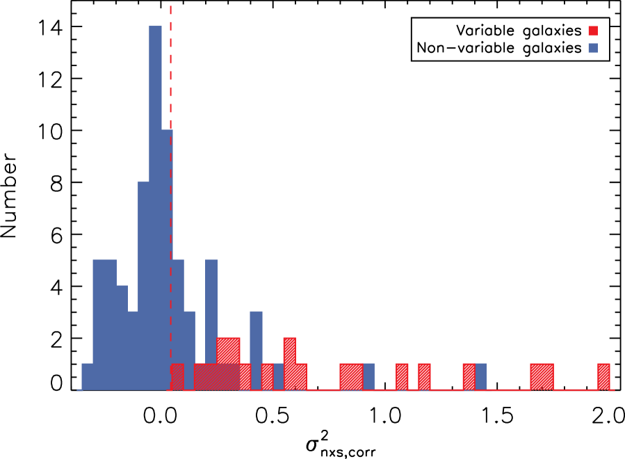
We find that XRB populations cannot explain the full extent of the X-ray variability for variable galaxies. Figure 8 plots the distribution of for CDF-S galaxies, showing that all the variable galaxies exhibit variability in excess of that expected from XRBs. The variable galaxies have a median / 42 (without the bias correction, /), indicating that the contribution of an XRB population to the measured variability is small.
We also consider whether one or more ultraluminous X-ray sources (ULXs) may dominate a galaxy’s X-ray output. The nature of ULXs is still debated, but most likely involves accretion onto massive stellar black holes (30–100 ); a few cases may involve accretion onto intermediate mass black holes (100–300 ) or beamed emission from 10–20 black holes. Typical luminosities span 1039–1041 ergs s-1 (e.g., Lehmer et al., 2006; Swartz et al., 2011). In a survey of 1,441 X-ray point sources in 32 nearby galaxies in the Chandra archive, Colbert et al. (2004) found ULXs in 19 galaxies; the contribution of one or more ULXs to a galaxy’s total X-ray point source luminosity ranged from 7%–87%, with a median contribution of 43%.
ULXs could potentially explain nine variable galaxies with ergs s-1. However, since ULXs tend to be associated with star-forming regions (e.g., Swartz et al., 2004) and occur more frequently in late-type/irregular galaxies than in early-type galaxies (e.g., Walton et al., 2011), the five variable galaxies with both ergs s-1 and late-type morphology (see §5.2) are more likely to host ULXs.
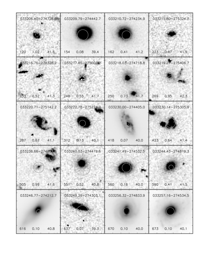
One method of finding ULXs is to search for off-nuclear sources. We plot postage-stamp images (8′′ 8′′) of the GOODS-S/GEMS HST -band for the variable galaxies in Figure 9. The circle overplotted on each image has a radius 1.5 times the Chandra positional erro, which is calculated at the 90% significance level. As in Lehmer et al. (2006), X-ray sources offset from the galaxy nucleus by more than 1.5 times the positional error are considered off-nuclear.
We find one marginally off-nuclear source: 033219.27275406.7 (XID = 269). The primary optical source appears to be an early-type galaxy with blending toward the galaxy to the lower right, suggesting a merger. Both galaxies have similar redshifts ( and 0.956, respectively); the first redshift is spectroscopic and secure (see §2) and the second is photometric (Xue et al., 2010). The high X-ray luminosity ( 2.21042 ergs s-1) suggests that a ULX is likely not the dominant source of X-ray emission from this galaxy.
One variable galaxy, 033230.00274405.0 (XID = 418), was previously identified as being off-nuclear in the 1 Ms CDF-S (Lehmer et al., 2006). With the additional data from the 4 Ms CDF-S, the X-ray source position has been refined (with reduced uncertainty) to be consistent with the galaxy’s nucleus. The off-nuclear source discussed in the previous paragraph (XID = 269) was not detected in the 1 Ms CDF-S, so it was not considered by Lehmer et al. (2006).
We cannot rule out that a ULX may lie too close to a galaxy’s nucleus to be detected as an off-nuclear source. However, the possibility of ULXs in most variable galaxies is mitigated by high X-ray luminosities and/or early-type morphology, so since we find no plausible off-nuclear ULXs, we conclude that ULXs are unlikely to dominate the emission from variable galaxies. Accretion onto a SMBH remains the best explanation of variable galaxies.
5. Supporting Evidence for LLAGN
We investigate the X-ray spectral shapes, the morphologies, and the optical spectral classifications of the variable galaxies for two purposes: (1) characterizing the variable galaxy population, and (2) determining whether their properties are consistent with those of LLAGN.
5.1. X-ray Spectral Shape
As discussed in §2, Xue et al. (2011) calculate the effective photon index for each source based on the ratio of count rates in the 2–8 keV and 0.5–2 keV bands (Table 2). For 10 variable galaxies detected in the soft band but not the hard band, lower limits are listed. For 4 low-count variable galaxies detected either in the full-band, soft-band, or both, no reliable effective photon index can be determined, so is set to 1.40.
Since 14 sources have poorly determined , we perform a stacking analysis on all variable galaxies with 150 net counts to determine an average photon index for the sample. The three highest count sources (with 199.2, 275.6, and 608.9 net counts) are excluded from the stacking analysis since they could dominate the stacked signal, but the results remain the same within errors if these sources are included.
Following the procedure in Luo et al. (2011), we calculate the soft and hard-band counts in a 3′′ diameter aperture for each source. The background is calculated by averaging the counts in 1,000 randomly placed, source-free apertures within a 1′-radius circle around the source position. The individual source counts are summed and background is subtracted. Aperture corrections are applied, averaged over all the observations weighted by exposure time (see Luo et al. 2011 for details), before calculating the band ratio.
The stacked effective photon index for the 17 relevant variable galaxies is 1.930.13, which is consistent with the typical photon index for local Seyfert galaxies ( 1.8; e.g., Dadina et al. 2008) at the 1 level. Including all 20 variable galaxies, 1.820.08. While absorption may still be present in some individual sources, the soft spectrum implied by the stacked effective photon index indicates that the average variable galaxy is not heavily obscured. The X-ray luminosities are therefore intrinsically low and indicate that variable galaxies are most likely LLAGN.
5.2. Galaxy Morphologies
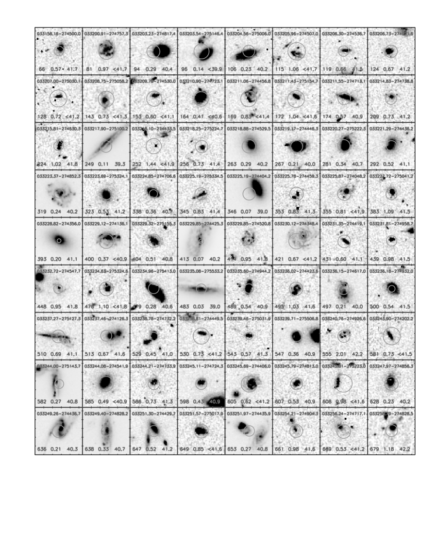
Postage-stamp images (8) of the GOODS-S/GEMS HST -band for CDF-S variable and non-variable galaxies are shown in Figures 9 and 10, respectively, with Chandra error circles overlaid. Galaxies are classified by eye as late-type, early-type, irregular, or undetermined. Mergers are also visually classified based on blending and/or tidal tails between two or more galaxies.
Since visual classifications are subjective and are particularly unreliable for distant, poorly resolved galaxies, we also apply the color-magnitude relation given in Bell et al. (2004), where galaxies are considered part of the “red sequence” (i.e., early-type morphology) if they are redder than ( – ) = -0.31 – 0.08 – 0.51. Galaxies with bluer colors are considered part of the ”blue cloud” (i.e., late-type morphology). Although the color-magnitude diagram leads to a more objective classification scheme, there are nevertheless significant uncertainties, both in the rest-frame magnitudes and colors, and in the definition of the Bell et al. (2004) relation. Moreover, the color classification is complicated by the fact that many of the galaxies lie in between the red sequence and blue cloud, in the so-called “green valley.” In cases where the color and the visually classified morphology disagree, we choose a final classification, preferring the visually classified morphologies in nearby, well-resolved galaxies, and the color classification in distant and/or poorly resolved galaxies. Considering only galaxies classified as early or late-type, the visual and color classifications agree 54% of the time. Table 2 lists each galaxy’s morphological type as determined by visual classification, the rest-frame magnitude and color (from Xue et al., 2011), the color classification according to Bell et al. (2004), and the final classification.
Based on the final classification from Table 2, we find that variability does not prefer one morphology type over the other. Variable galaxies have 40.0% early-type morphology and 50.0% late-type morphology, compared to 23.6% and 51.4%, respectively, in non-variable galaxies (the errors are 1 binomial errors). If we instead apply only the Bell et al. (2004) color classifications, then both the variable and non-variable galaxies prefer late-type morphologies (80.0% and 72.2%, respectively). The and SFR distributions for variable and non-variable galaxies show no significant difference ( 10%).
We find that the fraction of mergers among variable and non-variable galaxies is consistent within errors (% and %, respectively).
5.3. Optical Spectroscopic Classification
Most (18/20) variable galaxies have optical spectral observations (Szokoly et al., 2004; Zheng et al., 2004; Mignoli et al., 2005; Ravikumar et al., 2007; Popesso et al., 2009; Silverman et al., 2010), from which spectroscopic redshifts were determined. In all cases, the optical spectra are classified as galaxies, showing only narrow emission lines or absorption lines.
Szokoly et al. (2004) classify objects in more detail. Of the eight variable galaxies listed in the Szokoly et al. (2004) catalog, two have typical galaxy spectra showing only absorption lines. The remaining six are classified as having low-excitation emission lines consistent with H II region-type spectra. These objects would be classified as normal galaxies based on the optical data alone as the presence of the AGN cannot be established. However, one of these, 033222.78275224.2 (XID = 312), has sufficient signal-to-noise in the optical spectrum to measure line ratios. This object is classified as a LINER by Szokoly et al. (2004) via the line ratio diagnostics given by Ho & Sargent (1993).
6. Galaxy vs. AGN Variability
6.1. The Variability-Luminosity Anti-Correlation
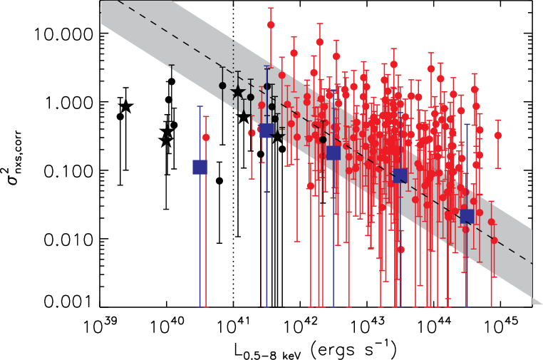
In this section, we investigate how galaxy variability compares to AGN variability. We first confirm a significant anti-correlation between excess variance and X-ray luminosity among AGN, as seen in previous work (e.g., Barr & Mushotzky, 1986; Lawrence & Papadakis, 1993; Nandra et al., 1997; Hawkins, 2000; Paolillo et al., 2004). The anti-correlation is plotted in Figure 11 for significantly variable sources as vs. . The excess variance includes the bias correction discussed in §4.1. The rest-frame X-ray luminosities are calculated differently for AGN and galaxies, as described in §2. The Spearman rank correlation coefficient ( = 0.44) shows the correlation is significant at 10-9 (5.9) for AGN only (red circles). The correlation increases in significance to () if all variable sources above = 1041 ergs s-1 are considered, including those classified as galaxies (black circles and stars). No significant correlation is found if the sample is limited to only the variable galaxies, which are discussed further in §6.2. Note that the correlation coefficient and best-fit line parameters (given below) remain consistent within errors if calculated using the excess variance uncorrected for sampling bias ().
Since both variability and luminosity may depend on other parameters, such as black hole mass and/or accretion rate, we fit the data using sixlin.pro, an IDL program adapted from Isobe et al. (1990). A least-squares bisector fit to sources with 1041 ergs s-1, weighted by the uncertainties in , results in = (25.82.6) . The slope and intercept are consistent within errors if the weights are not included. Large blue squares in Figure 11 show the weighted means for each luminosity bin; as expected, these are consistent with the weighted least-squares bisector. Note that since weighted means will most closely follow data with small error bars, they are weighted heavily downward in this log-log plot. Limiting the sample further to sources with 1042 ergs s-1 results in = (31.92.7) . The slopes are both consistent with the results of Nandra et al. (1997), where a weighted least-squares bisector fit results in (Nandra et al. 1997 do not give the normalization of their relation). This result is notable because the Nandra et al. (1997) data sampled shorter (hour–day) timescales compared to the months–years timescales sampled by the CDF-S.
The slope presented in this paper is significantly flatter than that found in Paolillo et al. (2004; ), which included non-varying sources. We choose not to include upper limits for non-varying sources in our analysis because the assumptions underlying survival analysis, which have been successfully applied to deal with censored data in other astronomical situations, do not apply here because: (1) the excess variance measurements of most sources lie near the detection limit, (2) a large percentage of sources do not have detected variability (50% of AGN and 78% of galaxies), and (3) a significant percentage of sources with no detected variability, especially those classified as galaxies, may truly not be variable (i.e., 0). By not including censored data in this paper’s measurements, we likely bias the measured slopes and possibly the significance of the anti-correlation. Nevertheless, the variability-luminosity anti-correlation has been observed to follow a model based on SMBH mass and accretion rate (e.g., Papadakis et al., 2008b), suggesting that the anti-correlation is real, though probably not linear. The model is discussed further in §6.3.
We check for other potential biases that may affect the luminosity-variability anti-correlation. The log-log plot of Figure 11 has the disadvantage of “hiding” sources with negative values. Sources with low flux values, and hence higher scatter in will therefore appear to have stronger variability, since the values scattered to negative values will be hidden. To check for this bias, we remove high scatter sources with () 0.1, excluding all but 38 sources, and find that the correlation remains significant at 0.9% (2.6). The best-fit slope and intercept remain consistent at the 1 level.
The flux-limited nature of the CDF-S survey presents another potential bias. Since luminosity correlates with redshift, and intrinsic variability timescales decrease with redshift, the decrease in variability strength as luminosity increases could, in principle, simply reflect the fact that shorter timescales are studied at higher redshifts, and therefore exhibit less variability due to the red-noise nature of AGN light curves. To check for a possible redshift bias, we examine the - correlation using a sub-sample within a narrow redshift range (0.55 0.75). This redshift range selects 10% of the total sample, covers luminosities from 1041.5 to ergs s-1, and results in minimal differences in rest-frame timescales. The Spearman rank correlation coefficient for this sub-sample remains significant at 0.8% (2.6); the slope and intercept are consistent at the 1 level.
The above test also addresses another potential bias due to the redshift range of the sample. The values listed in Table 2 measure the variability strength in the observed frame, so they will sample different energy bands depending on the source’s redshift (see §4.1 for discussion). This could introduce bias if the variablity amplitude changes with increasing energy: from keV at = 0 to keV at = 1. The slope and intercept remain the same within the narrow redshift range tested above, suggesting that any such bias does not have a significant effect on the sample.
6.2. Suppressed Variability in LLAGN
Variable sources with luminosities less than = 1041 ergs s-1 tend to fall significantly below the extrapolated linear relation by factors of 6–80 (median factor of 24), indicating a drop in variability relative to the linear relation on long timescales for LLAGN. This “suppressed” variability can be shown to be intrinsic to properties of AGN variability rather than due to dilution by unrelated XRB populations.
In §4.2, we showed that galaxy variability cannot be attributed solely to XRB populations. We now check whether the XRB contribution could nevertheless dilute the observed variability by estimating how much XRBs are expected to contribute to the total hard (2–10 keV), galaxy-wide X-ray luminosity (; see §4.2; Lehmer et al. 2010).
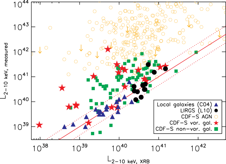
We compare to the measured, intrinsic X-ray luminosity. First, is converted to , using the intrinsic photon index of = 1.8 adopted by Xue et al. (2011) for AGN, and the stacked photon index 1.9 for galaxies (see §2). Figure 12 plots the measured 2–10 keV luminosity against that expected from an XRB population for variable galaxies (red stars) and non-variable galaxies (green squares). For reference, we plot in the same figure 369 CDF-S AGN (open orange circles), 32 local galaxies (Colbert et al., 2004), and 20 local luminous infrared galaxies, which are likely to be actively star-forming (Lehmer et al., 2010). The red solid line shows unity, while the dotted lines mark the dispersion observed in Lehmer et al. (2010).
A K-S test shows no significant difference between the relative XRB contribution in variable and non-variable galaxies. The CDF-S galaxies on average tend to lie above unity, with a median / 4.6. The X-ray excess in the non-variable galaxy population is perhaps not surprising given the flux-limited nature of the CDF-S survey, which is more likely to detect the objects at the bright end of the galaxy X-ray luminosity function, and may result in a high percentage of “contamination” by AGN.
The median X-ray excess for variable galaxies (/ 9.2) suggests that XRBs contribute 11% of the 2–10 keV luminosity for the average variable galaxy. For six variable galaxies, the total X-ray emission is consistent with that expected from XRB emission within the scatter of the Lehmer et al. (2010) relation (see Fig. 12), suggesting that dilution may be more significant in these sources. Three of these sources have variability consistent with the linear variability-luminosity relation, while three have suppressed variability (filled black stars in Fig. 11). Dilution by XRB variability may therefore play a role in suppressed variability, but cannot fully explain the extent to which is suppressed at low luminosities.
An alternative possible explanation for the suppressed variability at low luminosities is a change in accretion structure. Ptak et al. (1998) found a similar drop in variability strength below 21041 ergs s-1 in a sample of LLAGN and LINERs observed with ASCA on variability timescales of less than a day. The authors hypothesized that a radiatively inefficient accretion flow (RIAF, e.g., Yuan & Narayan 2004) could be responsible for suppressed short-timescale variability at low luminosities due to the larger extent of the X-ray source. This scenario would not obviously explain the reduced variability on month–year timescales seen here. RIAF models also predict a hard X-ray photon index due to the lack of an optically thick accretion disk, which provides the soft X-ray photons. The stacked X-ray photon index for variable galaxies ( 1.930.13; §5.1) is inconsistent with this prediction.
Studies since Ptak et al. (1998) have found evidence both for “suppressed” variability in LLAGN (e.g., Ptak et al., 2004; Markowitz & Uttley, 2005; Papadakis et al., 2008a) and against it (e.g., Binder et al., 2009; Pian et al., 2010). Similarly, objects such as narrow-line Seyfert 1 (NLS1) galaxies and the dwarf Seyfert NGC 4395 ( ) exhibit “excess” vairability for their luminosity (Boller et al., 1996; Iwasawa et al., 2010). However, when plotting variability against mass instead of luminosity (e.g., Papadakis et al., 2008a; Miniutti et al., 2009), such discrepancies disappear, with residual differences possibly due to varying accretion rates (e.g., McHardy et al., 2004; Markowitz & Uttley, 2005).
To investigate the role of SMBH mass () and accretion rate (normalized by the Eddington rate; = /), we have obtained rough estimates for all variable sources. Masses and Eddington ratios for all galaxies, variable and non-variable, are listed in Table 2. The SMBH masses are estimated via the scaling relation between and absolute -band magnitude (Graham, 2007):
| (7) |
The total absolute rest-frame -band magnitudes are derived from SED fitting in Xue et al. (2010) with a random scatter of 0.3 mag. An X-ray luminosity-dependent correction factor (Equation 1 of Vasudevan et al., 2009) corrects for nuclear emission. We assume that the host galaxy is bulge-dominated, a valid assumption for most AGN (e.g., Kauffman et al., 2003; Grogin et al., 2005). Several variable galaxies, however, are not bulge-dominated (nine are late-type; see Table 2), so their black hole masses may be overestimated. We apply a luminosity-dependent bolometric correction () to estimate the bolometric luminosity (Marconi et al., 2004) and calculate the Eddington ratio (/ [ ]/[ (/)]). Note, that the Marconi et al. (2004) correction is calculated explicitly for 1042 ergs s-1; we extrapolate this relation down to the lower luminosities of the variable galaxy sample.
Both the and estimation techniques are known to have large dispersions. The - scaling relation has a total scatter of 0.33 dex, and additional uncertainty will come from the luminosity-dependent correction for nuclear emission, which is based on template SEDs (Vasudevan et al., 2009). In addition, the assumption that all the variable galaxies are bulge-dominated will produce additional scatter.444The scaling relation in Kormendy & Gebhardt (2001), for example, has a much larger scatter of 0.56 dex largely because of poor bulge/disc separation (Graham, 2007). The bolometric correction, too, has large scatter due to the intrinsic dispersion in the SED. The uncertainty in due to SED dispersion is 20% for luminous AGN (Elvis et al., 1994; Richards et al., 2006). There is some debate regarding the similarity between the SEDs of LLAGN and luminous AGN (e.g., §1; Ho 1999 and Ho 2002 vs. Maoz et al. 2007); however, the luminous AGN SED dispersion likely serves as a lower limit to dispersion in LLAGN SEDs.
Variable galaxies tend to have lower accretion rates ( = 4 10-4) and masses () than variable AGN ( = 9 10-3; ), where we have limited the AGN sample to 1 for purposes of comparison. A K-S test shows that the differences in the and distributions are significant: PKS 1.710-5 and PKS 0.002, respectively. The properties of variable AGN and galaxies are consistent with the range of estimates made by Babic et al. (2007) for X-ray selected, 1 AGN in the 1 Ms CDF-S, which span 10 (median 0.001) and (median ).
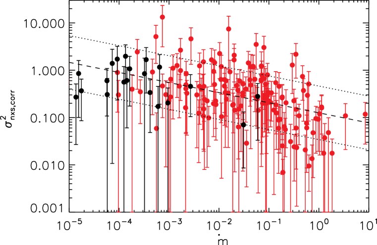
Unlike previous studies (O’Neill et al., 2005; Papadakis et al., 2008a; Miniutti et al., 2009), we find no significant (anti-)correlation between and , most likely due to the large scatter in and measurements, combined with the narrow range of masses probed (since most sources lie between 107–109 ). It is not surprising, therefore, that we find a significant anti-correlation between and (, ), plotted in Figure 13, which is likely an artefact of the – anti-correlation. Nevertheless, it is interesting that in Figure 13 the variable galaxies (black circles) connect smoothly with the more luminous AGN (red circles), with no discrepancy in variability strength. This suggests that the factor of 22.5 difference in may explain the “suppressed” variability in variable galaxies.
6.3. Comparing the Variability-Luminosity Relation with Empirical Models
A number of recent studies (e.g., McHardy et al., 2004; Papadakis, 2004; O’Neill et al., 2005; Papadakis et al., 2008b) have shown that X-ray variability may be determined by a combination of and , explaining the observed variability-luminosity relation. AGN light curves appear to be universally described by a broken power-law PSD function, where the break frequency depends on mass and accretion rate: (/)-1, where is the accretion efficiency, assumed to be (McHardy et al., 2006). The excess variance is equivalent to the integral of the PSD between the minimum and maximum frequencies sampled by the data, so as long as the break frequency falls within this range, the excess variance at a given luminosity will decrease with increasing and increase with increasing .
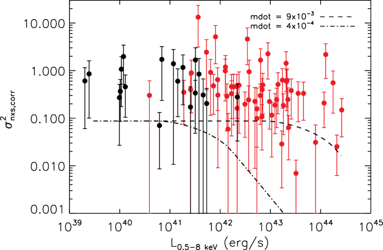
We compare the and values estimated in §6.2 to the variability measured for the variable AGN and galaxy populations. Assuming a universal PSD function, we derive the variability-luminosity relations expected for the CDF-S sampling pattern, given a range of SMBH masses and accretion rates (e.g., Papadakis et al., 2008b, and references therein). The bolometric luminosity, which is calculated directly from and , is converted to X-ray luminosity via a bolometric correction (Marconi et al., 2004). Where the break frequency lies outside the timescales sampled by the data (depending on the combination of and ), the excess variance will remain constant.
The model variability-luminosity relations are plotted in Figure 14 for the average accretion rates for variable ( = 9 10-3; dashed line) and non-variable ( = 4 10-4; dash-dotted line) galaxies covering = 105–10 (low to high ). Both variable populations are limited to 1 for comparison, and the relations are calculated at = 0.5 and = 0.7, the median redshifts for variable galaxies and AGN, respectively; using model redshifts = 0 or 1 resulted in negligible changes. The shape of the observed variability-luminosity anti-correlation, including the plateau at low luminosity, is roughly reproduced by the model. The plateau occurs when the break frequency lies outside the range of timescales sampled by the data. Unfortunately, the long timescales (especially the long minimum timescale of 4 Ms; see §4.1) and the large scatter prevent the models from distinguishing between the significantly different accretion rates estimated for variable galaxies and AGN.
Note that most sources are more variable than predicted by the model. We note some possible sources of bias: (1) The normalization of the PSD function used to calculate the models is based on a small sample of nearby AGN (Papadakis, 2004) and may therefore not be representative of CDF-S AGN out to . (2) Both the models and the bias correction applied to the measured excess variance (§4.1) depend on a universal broken power-law PSD function, but the slopes of the PSD may vary between individual sources, and some sources may even have a second break at shorter frequencies (e.g., McHardy et al., 2007). (3) Peculiar sources, such as NLS1s, exhibit higher variability555A notable exception is the NLS1 galaxy Akn 564, which is the only AGN observed to date to have a second, low-frequency break in its power spectrum, leading to lower variability on long timescales (McHardy et al., 2007)., so the variable sample may suffer from selection effects due to the higher sensitivity to more variable sources (§4.1).
7. Conclusions and Future Work
We have investigated the variability properties of sources classified as galaxies in the 4 Ms CDF-S by dividing the observations into 1 Ms epochs. We find the following main results:
1. Using a -based Monte Carlo simulation appropriate for low-count sources, 20 of 92 galaxies are selected as variable, as well as 185 of 369 AGN. Variability is effective in selecting AGN that do not meet other AGN selection criteria, such as cuts based on X-ray luminosity, X-ray-to-optical flux ratio, or excess X-ray emission compared to radio emission expected from star-forming galaxies (see §3). If all 20 variable galaxies are accreting SMBH, then the commonly used selection criteria employed by Xue et al. (2011) miss 20 of 389 AGN (5.1%), and 19 of 54 LLAGN (35.2%; where LLAGN are arbitrarily defined as having 1042 ergs s-1). Due to the low counts measured for most galaxies, it is likely that some non-variable galaxies may still host an AGN but not exhibit detectable variability, so these fractions serve as lower limits.
2. We measure variability strength with the normalized excess variance, accounting for measurement error, red-noise scatter, and bias due to the CDF-S sampling pattern. Comparing the bias-corrected excess variance to that expected from XRB populations, we find that XRBs cannot explain galaxy variability.
3. The possibility of energetically significant ULXs in variable galaxies is mitigated by high X-ray luminosities and/or early-type morphology. In addition, we find no plausible off-nuclear ULXs.
4. Galaxy X-ray variability is most likely associated with accretion onto a relatively unobscured SMBH. Though some absorption may be present, the individual and stacked photon indices show no indication of heavy obscuration and are consistent with the typical AGN spectral shape ( 1.930.13).
5. We confirm a significant anti-correlation between excess variance and X-ray luminosity, and find the slope and intercept to be consistent with what is reported in the literature for shorter timescales. We show that the sampling bias induced by the CDF-S observing pattern does not affect the anti-correlation slope or significance.
6. Low-luminosity sources ( 1041 ergs s-1, largely variable galaxies) have “suppressed” variability compared to the extrapolated linear relation between excess variance and X-ray luminosity. This may be explained by their lower accretion rates. Variable galaxies sample a different mass-accretion rate space than the rest of the AGN population, with significantly lower accretion rates ( = 4 10-4) and masses () than variable AGN ( = 9 10-3; ) in the same redshift range ().
7. We find that an empirical model based on a universal broken power-law PSD function, where the break frequency depends on SMBH mass and accretion rate, roughly reproduces the shape of the variability-luminosity anti-correlation. However, the normalization of the model is low compared to the data, suggesting systematic bias either within the data (e.g., selection effects) or the model (e.g., incorrect normalization for LLAGN at 1).
We have shown that the variability measured by deep X-ray surveys is an effective technique for selecting cosmologically distant LLAGN. Extending the CDF-S to even longer exposures would enable detection of variability in both fainter and less variable sources, thus allowing better characterization of the properties and abundance of the LLAGN population. Within the 4 Ms CDF-S, smaller time bins could be used to search for variability and better characterize the variability presented here.
In addition, follow-up optical spectroscopy is necessary to characterize the LLAGN population presented here. While Szokoly et al. (2004) were able to classify one object as a LINER, the spectra for the other sources did not have sufficient signal-to-noise to measure line ratios, so these objects would require either deeper optical spectroscopy or stacking of the currently available spectra.
References
-
Alexander et al. (2005)
Alexander, D. M., Bauer, F. E., Chapman, S. C., Smail, I., Blain, A.W., Brandt, W. N., & Ivison, R. J. 2005, ApJ, 632, 736
-
Alexander et al. (2008)
Alexander, D. M. et al. 2008, ApJ, 687, 835
-
(3)
Allevato, V. et al. 2011, in preparation
-
Almaini et al. (2000)
Almaini, O. et al. 2000, MNRAS, 315, 325
-
Babic et al. (2007)
Babic, A., Miller, L., Jarvis, M. J., Turner, T. J., Alexander, D. M. & Croom, S. M. 2007, A&A, 474, 755
-
Balestra et al. (2010)
Balestra, I., et al. 2010, A&A, 512, 12
-
Barr & Mushotzky (1986)
Barr, P. & Mushotzky, R. F. 1986, Nature, 320, 421
-
Barmby et al. (2006)
Barmby P. et al. 2006, ApJ, 650, L45
-
Barth et al. (1998)
Barth, A. J., Ho, L. C., Filippenko, A. V., & Sargent, W. L. W. 1998, ApJ, 496, 133
-
Bauer et al. (2004)
Bauer, F. E., Alexander, D. M., Brandt, W. N., Schneider, D. P., Treister, E., Hornschemeier, A. E., & Garmire, G. P. 2004, AJ, 128, 2048
-
Bell et al. (2003)
Bell, E. F., McIntosh, D. H., Katz, N., & Weinberg, M. D. 2003, ApJS, 149,289
-
Bell et al. (2004)
Bell, E. F., Wolf, C., Meisenheimer, K., Rix, H.-W., Borch, A., Dye, S., Kleinheinrich, M., Wisotzki, L.& McIntosh, D. H. 2004, ApJ, 608, 752
-
Binder et al. (2009)
Binder, B., Markowitz, A. & Rothschild, R. E. 2009, ApJ, 691, 431
-
Blundell et al. (1999)
Blundell, K. M., Rawlings, S., & Willott, C. J. 1999, AJ, 117, 677
- Boller et al. (1996) Boller, T., Brandt, W. N. & Fink, H. 1996, A&A, 305, 53
-
Boutsia et al. (2009)
Boutsia, K., Leibundgut, B., Trevese, D. & Vagnetti, F. 2009, A&A, 497,81
-
Brandt & Hasinger (2005)
Brandt, W. N. & Hasinger, G. 2005, ARA&A, 43, 827
-
Broos et al. (2010)
Broos, P. S., Townsley, L. K., Feigelson, E. D., Getman, K. V., Bauer, F. E., & Garmire, G. P. 2010, ApJ, 714, 1582
-
Caldwell et al. (2008)
Caldwell, J. A. R., et al. 2008, ApJS, 174, 136
-
Cameron (2011)
Cameron, E. 2011, PASA, 28, 128
-
Cardamone et al. (2010)
Cardamone, C. N., et al. 2010, ApJS, 189, 270
-
Colbert et al. (2004)
Colbert, E. J. M., Heckman, T. M., Ptak, A. F., Strickland, D. K. & Weaver, K. A. 2004, ApJ, 602, 231
-
Cooper et al. (2012)
Cooper, M. C. et al. 2012, MNRAS, submitted, arXiv:1112.0312
-
Dadina (2008)
Dadina, M. 2008, A&A, 485, 417
-
Damen et al. (2011)
Damen, M., et al. 2011, ApJ, 727, 1
-
Elvis et al. (1994)
Elvis, M. et al. 1994, ApJS, 95, 1
-
Ferrarese & Ford (2005)
Ferrarese, L. & Ford, H. 2005, Space Sci. Rev., 116, 523
-
Freeman et al. (2002)
Freeman, P. E., Kashyap, V., Rosner, R., & Lamb, D. Q. 2002, ApJS, 138, 185
-
Gallo et al. (2004)
Gallo, L. C., Boller, Th., Brandt, W. N., Fabian, A. C. & Vaughan, S. 2004, MNRAS, 355, 330
-
Gallo et al. (2007)
Gallo, L. C., Brandt, W. N., Costantini, E. & Fabian, A. C. 2007, MNRAS, 377, 1375
-
Gehrels (1986)
Gehrels, N. 1986, ApJ, 303, 336
-
Giavalisco et al. (2004)
Giavalisco, M., et al. 2004, ApJ, 600, L93
-
Gilfanov et al. (2004)
Gilfanov, M., Grimm, H. J. & Sunyaev, R. 2004, MNRAS, 351, 1365
-
Gilfanov (2010)
Gilfanov, M. 2010, LNP, 794, 17
-
Goncalves et al. (2008)
Goncalves, T. S., Steidel, C. C., & Pettini, M. 2008, ApJ, 676, 816
-
Gonzalez-Martin et al. (2011)
Gonzalez-Martin, O., Papadakis, I., Reig, P. & Zezas, A. 2011, A&A, 526, 132
-
Graham (2007)
Graham A. 2007, MNRAS, 379, 711
-
Grazian et al. (2006)
Grazian, A., et al. 2006, A&A, 449, 951
-
Grogin et al. (2005)
Grogin N. A. et al. 2005, ApJ, 627, 97
-
Gültekin et al. (2009)
Gultekin, K., et al. 2009, ApJ, 698, 198
-
Hawkins (2000)
Hawkins, M. R. S. 2000, A&A, 143, 465
-
Hickox & Markevitch (2006)
Hickox, R. C. & Markevitch, M. 2006, ApJ, 645, 95
-
Hopkins & Hernquist (2009)
Hopkins, P. F. & Hernquist, L. 2009, ApJ, 698, 1550
-
Hornschemeier et al. (2003)
Hornschemeier, A. E. et al. 2003, ApJ, 126, 575
-
Ho & Sargent (1993)
Ho, L. C., Filippenko, A. V., & Sargent, W. L. W. 1993, ApJ, 417, 63
-
Ho et al. (1997)
Ho, L. C., Filippenko, A. V., & Sargent, W. L. W. 1997, ApJS, 112, 315
-
Ho (1999)
Ho L. C. 1999, ApJ, 516, 672
-
Ho (2002)
Ho L. C. 2002, ApJ, 564, 120
- Houck et al. (2005) Houck, J. R. et al. 2005, ApJL, 622, 105
-
Isobe et al. (1990)
Isobe, T., Feigelson, E. D., Akritas, M. G. & Babu, G. J. 1990, ApJ, 364, 104
-
Iwasawa et al. (2010)
Iwasawa, K., Tanaka, Y. & Gallo, L. C. A&A, 514, 58
-
Jakobsen et al. (2003)
Jakobsen, P., Jansen, R. A., Wagner, S., & Reimers, D. 2003, A&A, 397,891
-
Kauffman et al. (2003)
Kauffmann, G., et al. 2003, MNRAS, 346, 1055
-
Kellerman et al. (1989)
Kellermann, K. I., Sramek, R., Schmidt, M., Shaffer, D. B. & Green, R. 1989, AJ, 98, 1195
-
Kormendy & Gebhardt (2001)
Kormendy J. & Gebhardt K., 2001, in Martel H., Wheeler J. C., eds, The 20th Texas Symposium on Relativistic Astrophysics. Am. Inst. Phys., New York, 586, 363
-
Kroupa (2001)
Kroupa, P. 2001, MNRAS, 322, 231
-
Komatsu et al. (2011)
Komatsu, E., et al. 2011, ApJS, 192, 18
-
Lawrence & Papadakis (1993)
Lawrence, A. & Papadakis, I. 1993, ApJ, 414, 85L
- Le Fèvre et al. (2004) Le F‘evre, O., et al. 2004, A&A, 428, 1043
-
Lehmer et al. (2006)
Lehmer, B. D., Brandt, W. N., Hornschemeier, A. E., Alexander, D. M., Bauer, F. E., Koekemoer, A. M., Schneider, D. P. & Steffen, A. T. 2006, AJ, 131, 2394
-
Lehmer et al. (2008)
Lehmer, B. D., et al. 2008, ApJ, 681, 1163
-
Lehmer et al. (2010)
Lehmer, B. D., Alexander, D. M., Bauer, F. E., Brandt, W. N., Goulding, A. D., Jenkins, L. P., Ptak, A. & Roberts, T. P. 2010, ApJ, 724, 559
-
Luo et al. (2008)
Luo, B., et al. 2008, ApJS, 179, 19
-
Luo et al. (2010)
Luo, B., et al. 2010, ApJS, 187, 560
-
Luo et al. (2011)
Luo, B., et al. 2011, ApJ, 740, 37
-
Marconi et al. (2004)
Marconi, M., Risaliti, G., Gilli, R., Hunt, L. K., Maiolino, R. & Salvati, M. 2004, MNRAS, 351, 169
- Markowitz & Uttley (2005) Markowitz A. & Uttley P. 2005, ApJ, 625, L39
-
McHardy et al. (2004)
McHardy, I. M., Papadakis, I. E., Uttley, P., Page, M. J. & Mason, K. O. 2004, MNRAS, 348, 783
-
McHardy et al. (2006)
McHardy, I. M., Koerding, E., Knigge, C., Uttley, P. & Fender, R. P. 2006, Nature, 444, 730
-
McHardy et al. (2007)
McHardy, I. M., Arèvalo, P., Uttley, P., Papadakis, I. E., Summons, D. P., Brinkmann, W. & Page, M. J. 2007, MNRAS, 382, 985
-
Maoz (2007)
Maoz, D. 2007, MNRAS, 377, 1696
-
Maoz et al. (2005)
Maoz, D., Nagar, N. M., Falcke, H. & Wilson, A. S. 2005, ApJ, 625, 699
-
Maoz et al. (1995)
Maoz, D., Filippenko,A.V., Ho, L.C., Rix, H.-W., Bahcall, J. N., Schneider,D. P., & Macchetto, F. D. 1995, ApJ, 440, 91
-
Martinez-Sansigre et al. (2005)
Martinez-Sansigre, A., Rawlings, S., Lacy, M., Fadda, D., Marleau, F., Simpson, C., Willott, C. J., & Jarvis, M. J. 2005, Nature, 436, 666
-
Mignoli et al. (2005)
Mignoli, M., et al. 2005, A&A, 437, 883
-
Miller et al. (2008)
Miller, N. A., Fomalont, E. B., Kellermann, K. I., Mainieri, V., Norman, C., Padovani, P., Rosati, P., & Tozzi, P. 2008, ApJS, 179, 114
- Miniutti et al. (2009) Miniutti, G., Ponti, G., Greene, J. E., Ho, L. C., Fabian, A. C. & Iwasawa, K. 2009, MNRAS, 394, 443
-
Morokuma (2008)
Morokuma, T. 2008, ApJ, 676, 121
-
Nandra et al. (1997)
Nandra, K., George, I. M., Mushotzky, R. F., Turner, T. J. & Yaqoob, T. 1997, ApJ, 476, 70
- O’Neill et al. (2005) O’Neill, Paul M., Nandra, K., Papadakis, I. E. & Turner, T. J. 2005, MNRAS, 358, 1405
-
Paolillo et al. (2004)
Paolillo, M., Schreier, E. J., Giacconi, R., Koekemoer, A. M., & Grogin, N. A. 2004, ApJ, 611, 93
-
Papadakis (2004)
Papadakis I. E. 2004, MNRAS, 348, 207
-
Papadakis et al. (2008a)
Papadakis, I. E., Ioannou, Z., Brinkmann, W. & Xilouris, E. M. 2008a, A&A, 490, 995
-
Papadakis et al. (2008b)
Papadakis, I. E., Chatzopoulos, E., Athanasiadis, D., Markowitz, A. & Georgantopoulos, I. 2008b, A&A, 487, 475
-
Peterson et al. (2006)
Peterson, K. C., Gallagher, S. C., Hornschemeier, A. E., Muno, M. P. & Bullard, E. C. 2006, AJ, 131, 133
-
Pian et al. (2010)
Pian, E., Romano, P., Maoz, D., Cucchiara, A., Pagani, C. & La Parola, V. 2010, MNRAS, 401, 677
-
Popesso et al. (2009)
Popesso, P., et al. 2009, A&A, 494, 443
-
Ptak et al. (1998)
Ptak, A., Yaqoob, T., Mushotzky, R., Serlemitsos, P. & Griffiths, R. 1998, ApJ, 501, 37L
-
Ptak et al. (2004)
Ptak, A., Terashima, Y., Ho, L. C. & Quataert, E. 2004, ApJ, 606, 173
-
Rafferty et al. (2011)
Rafferty, D. A., Brandt, W. N., Alexander, D. M., Xue, Y. Q., Bauer, F. E., Lehmer, B. D., Luo, B., & Papovich, C. 2011, ApJ, 742, 3
-
Ravikumar et al. (2007)
Ravikumar, C. D., et al. 2007, A&A, 465, 1099
- Richards et al. (2006) Richards, G.T. et al. 2006, ApJS, 166, 470
-
Sarajedini et al. (2011)
Sarajedini, V., Koo, D. C., Klesman, A. J., Laird, E. S., Perez Gonzalez, P. G. & Mozena, M. 2011, ApJ, 731, 97
-
Scheuer (1995)
Scheuer, P. A. G. 1995, MNRAS, 277, 331
-
Shankar et al. (2004)
Shankar, F., Salucci, P., Granato, G. L., De Zotti, G., & Danese, L. 2004, MNRAS, 354, 1020
-
Silverman et al. (2010)
Silverman, J. D., et al. 2010, ApJS, 191, 124
-
Supper et al. (1997)
Supper R., Hasinger G., Pietsch W., Trümper J. Jain A., Magnier E.A., Lewin W.H.G. & Van Paradijs J. 1997, A&A, 317, 328
-
Swartz et al. (2004)
Swartz, D. A., Ghosh, K. K., Tennant, A. F., & Wu, K. 2004, ApJS, 154, 519
-
Swartz et al. (2011)
Swartz, D. A., Soria, R., Tennant, A. F. & Yukita, M. 2011, ApJ, 741, 49
-
Szokoly et al. (2004)
Szokoly, G. P., et al. 2004, ApJS, 155, 271
-
Taylor et al. (2009)
Taylor, E. N., et al. 2009, ApJS, 183, 295
-
Timmer & Koenig (1995)
Timmer J. & Koenig M. 1995, A&A, 300, 707
-
Tozzi et al. (2001)
Tozzi, P., et al. 2001, ApJ, 562, 42
-
Treister et al. (2009)
Treister, E., et al. 2009, ApJ, 693, 1713
-
Trevese et al. (2008)
Trevese, D., Boutsia, K., Vagnetti, F., Cappellaro, E. & Puccetti, S. 2008, A&A, 488, 73
-
Vaughan et al. (2002)
Vaughan, S., Boller, T., Fabian, A. C., Ballantyne, D. R., Brandt, W. N., & Trumper, J. 2002, MNRAS, 337, 247
-
Vaughan et al. (2003)
Vaughan, S., Edelson, R., Warwick, R. S. & Uttley, P. 2003, MNRAS, 345, 1271
-
Vaughan et al. (2004)
Vaughan, S., Fabian, A. C., Ballantyne, D. R., De Rosa, A., Piro, L. & Matt, G. 2004, MNRAS, 351, 193
-
Vaughan & Fabian (2004)
Vaughan, S. & Fabian, A. C. 2004, MNRAS, 348, 1415
-
van den Bergh et al. (1973)
van den Bergh, S., Herbst, E. & Pritchet, C. 1973, AJ, 78, 375
-
Vanzella et al. (2008)
Vanzella, E., et al. 2008, A&A, 478, 83
-
Vasudevan et al. (2009)
Vasudevan, R. V., Mushotzky, R. F., Winter, L. M. & Fabian, A. C. 2009, MNRAS, 399, 1553
-
Villforth et al. (2010)
Villforth, C., Koekemoer, A. M. & Grogin, N. A. 2010, ApJ, 723, 737
-
Walton et al. (2011)
Walton, D. J., Roberts, T. P., Mateos, S. & Heard, V. 2011, MNRAS, 416, 1844
-
Weisskopf et al. (2007)
Weisskopf, M. C., Wu, K., Trimble, V., O’Dell, S. L., Elsner, R. F., Zavlin, V. E.,& Kouveliotou, C. 2007, ApJ, 657, 10
-
Xue et al. (2010)
Xue, Y. et al. 2010, ApJ, 720, 368
-
Xue et al. (2011)
Xue, Y. et al. 2011, ApJS, 195, 10
-
Younes et al. (2011)
Younes, G., Porquet, D., Sabra, B.& Reeves, J. N. 2011, A&A, 530, 149
-
Yuan & Narayan (2004)
Yuan, F. & Narayan, R. 2004, ApJ, 612, 724
-
Yun & Hibbard (2001)
Yun M. S. & Hibbard J. E. 2001, ApJ, 550, 104
-
Zheng et al. (2004)
Zheng, W., et al. 2004, ApJS, 155, 73
-
Zibetti et al. (2009)
Zibetti, S., Charlot, S. & Rix. H. W. 2009, MNRAS, 400, 1181
| Column | Description |
|---|---|
| 1 | Sequence number in the CDF-S catalog (Xue et al., 2011) (i.e., XID) |
| 2 | CDF-S name |
| 3 | Redshift |
| 4 | Method of redshift measurement (s = spectroscopic, p = photometric) |
| 5 | Upper limit flag for net counts |
| 6 | Total net counts in the 0.5–8.0 keV band or 3 upper limit |
| 7 | log (ergs s-1) |
| 8-10 | Effective photon index ()aaThe effective photon index is calculated from the band ratio. For sources detected in the soft band but not the hard band, is a lower limit. When the counts are too low to determine reliably the photon index from the band ratio, is set to 1.4. and corresponding errors |
| 11 | Variability statistic () |
| 12 | Probability that statistic is due to chance () |
| 13 | Maximum-to-minimum flux ratio () |
| 14-15 | Excess variance ()bbErrors on excess variance are calculated according to Equation (11) from Vaughan et al. (2003). The excess variance is not significant for non-variable galaxies, but the errors can be used to calculate an upper limit. and corresponding error |
| 16-17 | Bias-corrected excess variance (, see §4.1) and corresponding error |
| 18 | SFR ( yr-1) |
| 19 | (1010 ) |
| 20 | / |
| 21 | |
| 22 | Visual galaxy classification |
| 23 | |
| 24 | |
| 25 | Color galaxy classification |
| 26 | Final galaxy classification |
| 27 | log () |
| 28 | log / |
| XID | CDF-S name | aaFor 18 of 20 variable galaxies and 61 of 72 non-variable galaxies, the redshift is measured spectroscopically and is “secure” (see §2). The remaining galaxies have photometric redshifts. | Net | log | ||||||
|---|---|---|---|---|---|---|---|---|---|---|
| counts | ||||||||||
| 120 | 033206.40274728.6 | 1.02 | 32.7 | 41.62 | 1.4 | 2.8 | 0.0296 | 4.1 | 0.220.24 | 0.560.63 |
| 154 | 033209.79274442.7 | 0.08 | 46.9 | 39.39 | 0.9 | 2.9 | 0.0304 | 4.1 | 0.320.21 | 0.850.75 |
| 162 | 033210.72274234.9 | 0.42 | 111.7 | 41.16 | 1.0 | 5.8 | 0.0002 | 3.4 | 0.220.11 | 0.600.49 |
| 223 | 033215.80275324.7 | 0.67 | 43.7 | 41.51 | 1.0 | 5.4 | 0.0034 | 8.1 | 0.560.29 | 1.671.34 |
| 233 | 033216.76274328.2 | 0.52 | 61.0 | 41.26 | 1.0 | 4.4 | 0.0050 | 3.5 | 0.430.21 | 1.160.97 |
Note. — Table 2 is presented in its entirety in the electronic edition. A portion is shown here for guidance regarding its form and content. The full table contains 28 columns of information for the 20 variable and 72 non-variable CDF-S galaxies.
