Virial Sequences for Thick Discs and Haloes: Flattening and Global Anisotropy

Abstract

Stellar haloes and thick discs are tracer populations and make only a modest contribution to the overall gravity field. Here, we exploit the virial theorem to provide formulae for the ratio of the globally-averaged equatorial to vertical velocity dispersion of a tracer population in spherical and flattened dark matter haloes. This gives virial sequences of possible physical models in the plane of global anisotropy and flattening. The tracer may have any density distribution, although there are particularly simple results for power-laws and exponentials. We prove the Flattening Theorem: for a spheroidally stratified tracer density with axis ratio $q$ in equilibrium in a dark density potential with axis ratio $g$, the ratio of globally averaged equatorial to vertical velocity dispersion depends only on the combination $q/g$. As the stellar halo density and velocity dispersion of the Milky Way are accessible to observations, this provides a new method for measuring the flattening of the dark matter distribution in our Galaxy. If the kinematics of the local halo subdwarfs are representative, then the Milky Way’s dark halo model is oblate with a flattening in the potential of $g\approx 0.85$, corresponding to dark matter density contours with flattening $\approx 0.7$.

The fractional pressure excess for power-law populations is roughly proportional to both the ellipticity and the fall-off exponent. Given the same pressure excess, if the density profile of one stellar population declines more quickly than that of another, then it must be rounder. This implies that the dual halo structure claimed by Carollo et al. (2007) for the Galaxy – a flatter inner halo and a rounder outer halo – is inconsistent with the virial theorem.

For the thick disc, we provide formulae for the virial sequences of double-exponential discs in logarithmic and Navarro-Frenk-White (NFW) haloes. There are good matches to the observational data on the flattening and anisotropy of the thick disc if the thin disc is exponential with a short scalelength $\approx 2.6$ kpc and local surface density of $56\pm 6M_{\odot}{\rm pc}^{-2}$, together with a logarithmic dark halo. Thin discs with long scalelengths $\approx 3.5$ kpc are disfavoured. Likewise, Navarro-Frenk-White potentials do not seem to produce virial sequences matching the thick disc kinematics.

1 Introduction

The steady-state tensor virial theorem (see e.g. Chandrasekhar 1987) relates the overall geometry of the matter distribution to the global kinematics. It is a global result that constrains the components of the pressure, kinetic energy and potential energy tensors. The potential energy tensor $W_{ij}$ depends on the flattening, whilst the kinetic energy tensor $T_{ij}$ describes the rotational and velocity anisotropy properties.

Stars and their kinematics provide one of the tools available for studies of the morphologies and sizes of galaxies and their halos. So, a classic application of the tensor virial theorem is to the problem of the shape of elliptical and lenticular galaxies. Binney (1978, 2005) gave a pictorial representation of the plane of ellipticity $\epsilon$ versus ratio of rotational to pressure support $v/\sigma$ for early-type galaxies. He showed that if elliptical galaxies have isodensity surfaces that are similar ellipsoids, then $v/\sigma$ is completely determined by the velocity anisotropy and the flattening. This diagram is an important tool in understanding whether the flattening of an elliptical galaxy is due to velocity anisotropy or rotation.

Although the tensor virial theorem has been widely used in galactic astronomy, applications have been largely confined to self-gravitating systems – such as the stars in bulges or elliptical galaxies — which are moving in a potential mainly generated by their own density field. However, some populations make a very modest contribution to the total potential in which they move. An example is the population of metal-poor halo stars, which are mere tracers of the gravity field of the overwhelmingly dominant dark halo. Similarly, the stars of the thick disc move in the combined field of the more massive thin disc and dark halo. We shall refer to such instances as tracer populations. Here, we provide a systematic investigation of the tensor virial theorem applied to tracers, including stellar haloes and thick discs.

Conventional methods of analysis of stellar kinematical data on tracer populations are usually based upon phase space distribution functions (e.g, Evans, Hafner & de Zeeuw 1997, Deason, Evans & Belokurov 2011a) or upon the Jeans equations (e.g., van der Marel 1991, Battaglia et al. 2005). The former is most fundamental as it is equivalent to solving the collisionless Boltzmann equation. The method usually depends upon an Ansatz as to the likely phase space distribution function, with the free parameters fit in a maximum likelihood sense to the kinematical data. The latter is less fundamental, as the Jeans equations are moments of the collisionless Boltzmann equation. The method depends not just on the stellar density and velocity field, but also explicitly on their gradients, which are hard to obtain with noisy data and susceptible to deviations caused by contaminants, interlopers and substructure.

The tensor virial theorem is obtained by integration of moments of the Jeans equations, and so can be regarded as a globally averaged version of them. Although there are earlier attempts to use the tensor virial theorem to study properties of the Galaxy via the kinematics of tracer stars in the literature (White 1989, Sommer-Larsen & Christensen 1989), they were held up by a serious drawback. Kinematic quantities, for example, of halo stars in our Galaxy are only known locally, and there is a leap of faith required in extrapolating from local to global quantities. However, given the many large scale surveys of Galactic stars underway or planned, it is now worthwhile to examine the tensor virial theorem anew for its potentiality. Astrometric satellites such as GAIA (Turon et al. 2005), current spectroscopic surveys such as SEGUE (Yanny et al. 2009), and forthcoming initiatives, such as ESO-GAIA and Hermes, offer the prospects of huge amounts of kinematic information becoming available for many stars throughout the Galaxy. Understanding these complex and overlapping datasets, and extracting useful information from the radial velocities and proper motions, will be a major task over the next few years. Global averages like the tensor virial theorem may provide a quick way of extracting ready and accurate information on the structure of the Galactic potential.

The paper is arranged as follows. In Section 2, we introduce the tensor virial theorem. Section 3 derives formulae for the ratio of equatorial to vertical pressure for scale-free tracer populations in spherical haloes. In Section 4, we develop theorems that extend our results to the cases of flattened haloes and more general tracer populations. Section 5 discusses applications to Population II stars in the stellar halo of the Milky Way. Using observational data on the pressure ratio, we develop a new method of constraining the flattening of the dark halo. We also show that virial arguments impose strong constraints on multiple populations moving in the same potential and apply our arguments to recent claims of duality in the stellar halo. Section 6, discusses applications to the thick disc, in particular focusing on whether the observed kinematics and flattening are consistent with motion in a thin disc potential with short or long scalelength. Finally, we revisit the stellar halo in Section 7, asking whether it is conceivable that the flattening to the potential provided by the thin disc alone reproduce the observed flattening and kinematics.

2 The Tensor Virial Theorem

Let $V$ be the volume of our survey. For an all-sky survey like GAIA, $V$ might be all space. However, this need not always be the case.

Whatever the volume $V$, the kinetic energy tensor $K_{ij}$ is the sum $2T_{ij}+\Pi_{ij}$, where

$$T_{ij} = \frac{1}{2}\int_{V}{\rho{\bar{v}_{i}}{\bar{v}_{j}}}\mathrm{d}^{3}x,$$ (1)

$$\Pi_{ij} = \int_{V}{\rho\sigma^{2}_{ij}}\mathrm{d}^{3}x.$$ (2)

Here, $\rho$ is the stellar density, whilst ${\bar{v}_{i}}$ is the velocity field and $\sigma^{2}_{ij}$ is the velocity dispersion tensor. Here, an overbar denotes an average over the velocity distribution so that

$$\sigma^{2}_{ij}=\overline{(v_{i}-{\bar{v}_{i}})(v_{j}-{\bar{v}_{j}})}.$$ (3)

We note that $T_{ij}$ is the kinetic energy in ordered, rotational motion (often negligible for stellar halos but substantial for thick discs), whilst $\Pi_{ij}$ is the pressure tensor. The potential energy tensor is

$$W_{ij} = \int_{V}\rho x_{i}{\partial\Phi\over\partial x_{j}}\mathrm{d}^{3}x\ ,$$ (4)

where $\Phi$ is the gravitational potential.

To obtain the relationship between these tensors, we start from the steady-state Jeans equations, which read

$${\partial\over\partial x_{k}}\rho\overline{v_{k}v_{j}}=-\rho{\partial\Phi\over\partial x_{j}}\ .$$ (5)

Multiplying by $x_{i}$, integrating over the volume $V$ and making use of the divergence theorem gives the steady-state, tensor virial theorem (e.g., Chandrasekhar 1987, Binney 1981)

$$K_{ij}+W_{ij}=2T_{ij}+\Pi_{ij}+W_{ij}=S_{ij}\ ,$$ (6)

where the surface term is

$$S_{ij}=\oint_{\partial V}x_{i}\rho\overline{v_{j}v_{k}}dS_{k}\ ,$$ (7)

and $\partial V$ is the bounding surface. If the integration volume $V$ is taken as all space, then the surface term can be discarded provided that the pressure $\rho\overline{v_{j}v_{k}}$ falls off more quickly than $r^{-3}$.

For an axisymmetric density and potential, we will often find it convenient to use cylindrical polars ($R,\phi,z$). It is useful to sum up all the kinetic energy or pressures in the equatorial plane and refer to

$$K_{RR}=K_{xx}+K_{yy},\qquad\qquad\Pi_{RR}=\Pi_{xx}+\Pi_{yy}.$$ (8)

Analogously, we can also introduce

$$W_{RR}=W_{xx}+W_{yy}\ =\ \int{\rho R\partial_{R}\Phi}\mathrm{d}^{3}x$$

and $S_{RR}=S_{xx}+S_{yy}$.

The great advantage of virial methods is that integrated quantities (such as total kinetic energy of the stars in the survey volume) can in general be evaluated robustly even with quite sparse data. A price to be paid is that the surface terms may not necessarily vanish and may have to be evaluated from the data.

3 Tracer Populations in Spherical Dark Haloes

For the moment, the gravitational potential is assumed to be dominated by dark matter. The stars comprise a tracer population. This assumption is fine for stellar haloes which move in the dominating dark matter potential. For example, the Milky Way Galaxy’s stellar halo has a total mass of $\sim 4\times 10^{8}{M_{\odot}}$ (e.g., Bell et al. 2008), which is four orders of magnitude smaller than the dark matter halo (e.g., Watkins et al. 2010).

3.1 The Pressure Ratio

Let us take the potential to be spherically symmetric (i.e. $\Phi(x,y,z)\equiv\Phi(r)$) and the stellar density to be axisymmetric (i.e., $\rho(x,y,z)\equiv\rho(R,z)$). Let the integration volume $V$ be over all space and let the surface terms vanish, so that the tensor virial theorem can be manipulated to yield:

$${\displaystyle K_{RR}\over\displaystyle K_{zz}}=\ {\displaystyle\int{\rho R^{2}\Phi^{\prime}\over\displaystyle r}\mathrm{d}^{3}x\over{\displaystyle\int{\rho z^{2}\Phi^{\prime}\over\displaystyle r}\mathrm{d}^{3}x}}\ ,$$ (9)

where $\Phi^{\prime}=\mathrm{d}\Phi/\mathrm{d}r$. The quantity ${K_{RR}/K_{zz}}$ is the ratio of the equatorial or in-plane kinetic energy to the vertical kinetic energy.

Stellar haloes are only weakly rotating (e.g., Deason et al. 2011a), so it is to fair to assume that there is no mean streaming motion ($T_{ij}=0$). Then, ${K_{RR}/K_{zz}}$ is the same as ${\Pi_{RR}/\Pi_{zz}}$, the ratio of pressure in the equatorial to vertical directions. For an axisymmetric figure, it is natural to expect this to be intimately related to the flattening.

3.2 Scale-Free Spheroidal Densities

To begin with, let us assume that the tracer density is scale-free and has the form

$$\rho={f(\theta)\over r^{\gamma}}$$ (10)

where ($r,\theta$) are spherical polars and $\gamma$ is the power-law fall-off. Formally, the scale-free density is non-integrable either at the origin or at infinity and so the virial quantities do not exist. Nonetheless, their ratio is well-defined and given by

$${\displaystyle W_{RR}\over\displaystyle W_{zz}}={\displaystyle\Pi_{RR}\over\displaystyle\Pi_{zz}}={\displaystyle\int_{0}^{\pi}f(\theta)\sin^{3}\theta\mathrm{d}\theta\over\displaystyle\int_{0}^{\pi}f(\theta)\sin\theta\cos^{2}\theta\mathrm{d}\theta}\ .$$ (11)

As an illustration, we specialise to the case in which the tracer density is stratified on similar concentric spheroids as

$$\rho=\rho_{0}\left(R^{2}+z^{2}q^{-2}\right)^{-\gamma/2},$$ (12)

with ($R,\phi,z$) familiar cylindrical polar coordinates. Here, $q$ is the axis ratio of the equidensity contours, which is simply related to the ellipticity $\epsilon=1-q$. The virial ratio eq (11) is

$${\displaystyle W_{RR}\over\displaystyle W_{zz}}={\displaystyle\Pi_{RR}\over\displaystyle\Pi_{zz}}={\displaystyle\int_{0}^{\pi}\sin^{3}\theta(\sin^{2}\theta+q^{-2}\cos^{2}\theta)^{-\gamma/2}\mathrm{d}\theta\over\displaystyle\int_{0}^{\pi}\sin\theta\cos^{2}\theta(\sin^{2}\theta+q^{-2}\cos^{2}\theta)^{-\gamma/2}\mathrm{d}\theta}\ ,$$ (13)

which is independent of $\Phi$

Some simple and useful results can be obtained in the case of modest flattening, $q\rightarrow 1$. Using the shorthand $Q=q^{-2}$, then Taylor expansion yields

$${\displaystyle\Pi_{RR}\over\displaystyle\Pi_{zz}}={\displaystyle\int_{0}^{\pi}\sin^{3}\theta(1-{{1\over 2}}\gamma[Q-1]\cos^{2}\theta)\mathrm{d}\theta\over\displaystyle\int_{0}^{\pi}\sin\theta\cos^{2}\theta(1-{{1\over 2}}\gamma[Q-1]\cos^{2}\theta)\mathrm{d}\theta}.$$ (14)

We can get an expression for the vertical and horizontal pressure difference by making the definitions $\langle\sigma^{2}_{zz}\rangle=\Pi_{zz}/M$ and $\langle\sigma^{2}_{xx}\rangle=\frac{1}{2}\Pi_{RR}/M$, where $M$ is the total mass of the tracer population. The angled brackets therefore denote mass-weighted averages of the velocity dispersions. We can now recast eq (14) as

$$\frac{\langle\sigma^{2}_{xx}\rangle}{\langle\sigma^{2}_{zz}\rangle}\ \approx 1+{\gamma\over 5}(Q-1)+{3\gamma(\gamma-5)\over 175}(Q-1)^{2}.$$ (15)

Bearing in mind that $Q=1/q^{2}=1/(1-\epsilon)^{2}$, where $\epsilon$ is the ellipticity, we see that the fractional pressure excess is

$$\frac{\langle\sigma^{2}_{xx}\rangle-\langle\sigma^{2}_{zz}\rangle}{\langle\sigma^{2}_{zz}\rangle}\ \approx{1\over 5}\gamma(Q-1)\approx{2\over 5}\gamma\epsilon\ .$$ (16)

In other words, for a mildly flattened stellar halo with a given ellipticity and power-law density fall-off residing in a spherical dark halo, then

$${\rm Fractional\ pressure\ excess}\approx{2\over 5}\times{\rm Falloff}\times{\rm Ellipticity}\ .$$ (17)

We note that, when $\langle\sigma^{2}_{xx}\rangle\rightarrow\langle\sigma^{2}_{zz}\rangle,$ $Q$ and hence $q$ tend to $1$ (i.e. the stellar halo is spherically stratified), and vice-versa. This behaviour in the isotropic pressure limit is general for spherical dark matter haloes.

In the limit of extreme flattening, an asymptotic expansion of eq (13) yields

$$\frac{\Pi_{RR}}{\Pi_{zz}}\sim\begin{cases}(\gamma-3)q^{-2}&\text{if $\gamma>3$}\\ q^{-2}/\log(2q^{-2})&\text{if $\gamma=3$}\\ \frac{1}{2}(3\!-\!\gamma)q^{1-\gamma}B(\frac{\gamma\!-\!1}{2},\frac{\gamma}{2})&\text{if $1<\gamma<3$}\end{cases}$$ (18)

with $B(a;b)=\Gamma(a)\Gamma(b)/\Gamma(a+b)$ being the Beta function. Stellar halo populations typically have $\gamma\gtrsim 3$ and so the pressure ratio $\Pi_{RR}/\Pi_{zz}\sim q^{-2}$ for high flattening. We will see later in Section 6 how the presence of a thin disc alters this behaviour.

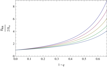
Figure 1: Virial sequences for spheroidal stellar halos. The pressure ratio ${{1\over 2}}\Pi_{RR}/\Pi_{zz}$ is shown as a function of the flattening $q$ for stellar densities with fall-off $\gamma=3$ (blue), 3.5 (green), 4 (yellow), 4.5 (red) and 5 (purple). The pre-factor of ${{1\over 2}}$ means that the vertical axis is $\Pi_{xx}/\Pi_{zz}$ and ensures that the ratio tends to unity as $q\rightarrow 1$. The analytic form of these curves is given in eqs (20), (21) and (22) for $\gamma=3$, 4 and 5.

3.3 Exact Results

In fact, the pressure ratio in eq (13) is analytic in the case that power-law fall-off $\gamma$ is an integer. It is helpful to have the exact expressions. For $\gamma=2$, we find:

$${\Pi_{RR}\over\Pi_{zz}}=\ \frac{Q\arctan\sqrt{Q-1}-(Q-1)^{{1\over 2}}}{(Q-1)^{{1\over 2}}-\arctan\sqrt{Q-1}}.$$ (19)

For the case $\gamma=3$, we have:

$$\frac{\Pi_{RR}}{\Pi_{zz}}\ =\ \frac{(Q-1)^{{{3\over 2}}}-\sqrt{Q}{\rm arcsinh}\sqrt{Q-1}+(Q-1)^{{1\over 2}}}{\sqrt{Q}{\rm arcsinh}\sqrt{Q-1}-(Q-1)^{{1\over 2}}}\ .$$ (20)

This formula is equivalent to one derived by White (1989) for populations orbiting in an isothermal sphere.

The $\gamma=4$ case has already been discussed by Helmi (2008). We find:

$$\frac{\Pi_{RR}}{\Pi_{zz}}\ =\ \frac{Q(Q-2)\arctan\sqrt{Q-1}+(Q-1)^{{1\over 2}}}{Q\arctan\sqrt{Q-1}-(Q-1)^{{1\over 2}}}\ .$$ (21)

Like us, Helmi assumes that the stellar halo is flattened and follows a scale-free power-law density, whilst the dark halo is spherical. In fact, Helmi specialises to the particular case of a logarithmic potential generating an asymptotically flat rotation curve. To make progress, Helmi makes an additional assumption, namely that the ratio of horizontal to vertical velocity dispersions $\sigma_{x}^{2}/\sigma_{z}^{2}$ does not depend on location. Unfortunately, the final formula – equation (8) of Helmi (2008) – contains two mistakes. The first is computational, namely the integrals are incorrect. This can be seen by noting that, in the limit of a spherical stellar halo ($Q\rightarrow 1$), the velocity dispersion tensor must become isotropic within Helmi’s set of assumptions, a fact that is contradicted by her formula. The second is more subtle and conceptual. The ratio $\sigma_{x}^{2}/\sigma_{z}^{2}$ between velocity dispersions in the $x$ and $z$ coordinates cannot be considered uniform, once the density and potential profiles are already assigned: this additional assumption over-determines the problem.

For the $\gamma=5$ case, the result is exceptionally simple, namely

$$\frac{\Pi_{RR}}{\Pi_{zz}}\ =2Q={2\over q^{2}}.$$ (22)

The result is exact for arbitrary flattening.

Figure 1 shows the behaviour of $\Pi_{xx}/\Pi_{zz}$ valid for any spherical potential. It assumes a power-law profile for the stellar density stratified on similar concentric spheroids with axis ratio $q$ and with density fall-off $m$ varying between 3 (lower curve) and 5 (upper curve). Populations in the stellar halo typically fall off like $r^{-3}$ or $r^{-4}$, though some variable star populations such as RR Lyrae (e.g., Watkins et al. 2009) and Miras (e.g., An et al. 2004) can fall off faster. As a general rule, the faster the density fall-off, and the greater the flattening, then the larger the pressure excess needed to support the stellar distribution.

3.4 Alignment of the Velocity Ellipsoid

To make practical use of the virial formulae, we must find the connection between the pressure ratio and the velocity dispersions. This is straightforward if the velocity dispersion tensor is diagonal in cylindrical polar coordinates, namely

$${\Pi_{RR}\over\Pi_{zz}}={\displaystyle\int\rho(\sigma^{2}_{RR}+\sigma^{2}_{\phi\phi})\mathrm{d}^{3}x\over\displaystyle\int{\rho\sigma^{2}_{zz}\mathrm{d}^{3}x}}\ .$$ (23)

If the velocity dispersion tensor is aligned in spherical polar coordinates – as is the case for halo stars (e.g., Smith et al. 2009b) – then matters are more complicated. The diagonal components of the velocity dispersion tensor in cylindrical polar coordinates are now given by

$$\sigma_{RR}^{2} =\sigma_{rr}^{2}\sin^{2}\!\theta+\sigma_{\theta\theta}^{2}\cos^{2}\!\theta=(1-\beta\cos^{2}\!\theta)\,\sigma_{rr}^{2}$$ (24a)

$$\sigma_{\phi\phi}^{2} =\sigma_{\theta\theta}^{2}=(1-\beta)\,\sigma_{rr}^{2}$$ (24b)

$$\sigma_{zz}^{2} =\sigma_{rr}^{2}\cos^{2}\!\theta+\sigma_{\theta\theta}^{2}\sin^{2}\!\theta=(1-\beta\sin^{2}\!\theta)\,\sigma_{rr}^{2}$$ (24c)

where $\beta$ is the anisotropy parameter,

$$\beta=1-{\sigma_{\theta\theta}^{2}\over\sigma_{rr}^{2}}\ .$$ (25)

This means that

$${\Pi_{RR}\over\Pi_{zz}}={\displaystyle\int\rho\sigma^{2}_{rr}(2-{\beta}+{\beta}\cos^{2}\theta)\mathrm{d}^{3}x\over\displaystyle\int{\rho\sigma^{2}_{rr}(1-\beta\sin^{2}\theta)\mathrm{d}^{3}x}}\ .$$ (26)

If $\beta$ is constant, this simplifies to

$${\Pi_{RR}\over\Pi_{zz}}={\displaystyle(2-\beta)\langle\sigma^{2}_{rr}\rangle-\beta\langle\sigma^{2}_{rr}\cos^{2}\theta\rangle\over\displaystyle\langle\sigma^{2}_{rr}\rangle-\beta\langle\sigma^{2}_{rr}\sin^{2}\theta\rangle}$$ (27)

where angled brackets denote mass-weighted averages. If the tracer flattening is known and the variation of the velocity dispersions is estimated over the survey volume, eq (27) yields virial sequences that do not involve the potential $\Phi$. Thus, we can constrain the potential by intersecting the $W_{RR}/W_{zz}$ sequences with the pressure ratios. Nonetheless, practical application of eq (27) is limited by the fact that the global variation of the dispersions with position is not well understood, though this will be remedied after the next generation of large-scale surveys of the Milky Way (such as GAIA).

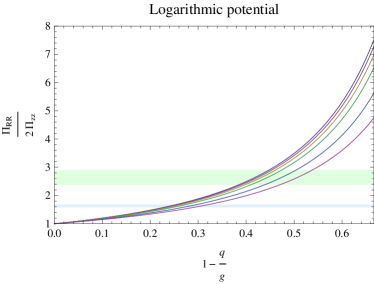
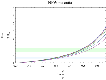
Figure 2: Virial sequences for the stellar halo density law found by Deason et al. (2011b) and given in eq. (39). The pressure ratio ${{1\over 2}}\Pi_{RR}/\Pi_{zz}$ is shown as a function of flattening ratio $q/g$, where $q$ is the axis ratio of the stellar density contours and $g$ is the axis ratio of the dark matter equipotentials. The dark matter potential has a logarithmic form generating a flat rotation curve (left) and a NFW dark matter halo (right). The coloured lines refer to different values of the dark matter scalelength from $5$ kpc (lower red curve) through 15 kpc, 35 kpc, 55 kpc, 75 kpc to $95$ kpc (upper blue curve) and taking the break radius fixed at ${R_{\rm b}}=27$ kpc (Deason et al. 2011b). The green and blue bands give the range in pressure ratios found by global extrapolation of the local results of Kepley et al. (2007) and by Smith et al. (2009a).

4 Two Theorems

4.1 The Flattening Theorem

If our formulae were restricted to spherical dark haloes, they would have limited applicability. Here, we derive a remarkable theorem that extends our results to the case of flattened tracer populations in flattened dark haloes.

Let the tracer density and total potential satisfy the following requirements

$$\rho(R,qz)=\rho(qz,R),\qquad\qquad\Phi(R,gz)=\Phi(gz,R),$$ (28)

for some $q$ and $g$. We say in this case that $\rho$ and $\Phi$ are stratified on constant flattening surfaces. The above definition is equivalent to requiring that $\rho$ (or $\Phi$) be a symmetric function of $R$ and $z/q$ (or $z/g$). The most commonly used examples are spheroidal distributions, such as

$$\Phi=\Phi(m),\qquad\qquad m^{2}=R^{2}+z^{2}g^{-2}.$$ (29)

There are a number of popular halo models of this form, including Binney’s (1978) logarithmic potential and the power-law models (Evans 1993, 1994). The dark matter density may be cored or cusped. The flattening, or the minor to major axis ratio, of the dark matter equipotentials $g$ is rounder than the dark matter isodensity contours. Similarly, the spheroidal power-law densities with fall-off $\gamma$ and axis ratio $q$ studied in the previous section belong to this class, though there are many other possibilities for the tracer density as well.

In what follows, it is convenient to specialize to spheroidally stratified potentials with flattening $g$. The tensor virial theorem becomes:

$${\displaystyle\Pi_{RR}\over\displaystyle\Pi_{zz}}=\ {\displaystyle\int{\rho R\partial_{R}\Phi}\mathrm{d}^{3}x\over{\displaystyle\int{\rho z\partial_{z}\Phi}\mathrm{d}^{3}x}}\ =\ {\displaystyle\int{\rho R^{2}\Phi^{\prime}\over m}\mathrm{d}^{3}x\over{\displaystyle\int{\rho g^{-2}z^{2}\Phi^{\prime}\over m}\mathrm{d}^{3}x}}\ ,$$ (30)

where $\Phi^{\prime}=\mathrm{d}\Phi/\mathrm{d}m$.

Making the substitution $z=z^{\prime}g,$ writing $r^{\prime 2}=x^{2}+y^{2}+z^{\prime 2}$ and then dropping the primes, the integrals on the right-hand side of eq (30) are converted into the exact form as those on the right-hand side of eq (9), with the only change

$$\rho(R,z/q)\rightarrow\rho(R,gz/q).$$ (31)

This means that all our preceding results for spherical haloes hold good in the flattened case, but with the replacement

$$q\rightarrow q/g.$$ (32)

This considerably extends the scope of our earlier results.

More formally, our theorem can be stated as follows. If the dark matter potential $\Phi$ is homoeoidally stratified with flattening $g$ and the tracer density $\rho$ has a constant flattening $q$, then the virial ratio $W_{RR}/W_{zz}$ depends on the two flattenings just through their ratio $q/g$.

As a corollary, for scale-free densities with constant flattening the virial ratios depend on $q/g$ and the power-law exponent, but not on the radial form of the potential, as already noticed for spherical potentials. This can be seen by using spherical polar coordinates and noting that the radial integrals (containing $\Phi$) factorize and cancel top and bottom. The angular integrals do depend on the density stratification and the behaviour of $W_{RR}/W_{zz}$, and thence $\Pi_{RR}/\Pi_{zz}$, is controlled by those:

$${\Pi_{RR}\over\Pi_{zz}}=\ {\displaystyle\int{\rho(\sin\theta,(g/q)\cos\theta)\sin^{3}\theta}\mathrm{d}\theta\over\displaystyle\int{\rho(\sin\theta,(g/q)\cos\theta)\cos^{2}\theta\sin\theta}\mathrm{d}\theta}\ .$$ (33)

As a consequence, once a virial ratio has been computed for a spherical dark matter potential, the flattened analogue follows in a straightforward manner. Providing the potential remains spheroidally stratified, any halo model such as isothermal or Navarro-Frenk-White (1998) or Sersic (1963) is fine. This is an extension of a famous and elegant result from potential theory due to Roberts (1962), which states that ratios such as $W_{RR}/W_{zz}$ depends only on the axial ratios for homoeoidal distributions, and not on the radial profiles.

The ratio $W_{RR}/W_{zz}$ does depend on the form of $\Phi$, if more complex profiles are prescribed, for example, accounting for the contribution of the stellar disc, or the differential flattening of the dark matter halo and the self-gravity of the stellar halo. However, although analytic progress is difficult for complex profiles, the relevant integrals are easily evaluated numerically.

4.2 The Conjugateness Theorem

As shown above, there is a class of test densities (like scale-free ones) yielding virial ratios that are independent of the radial behaviour of $\Phi$. Similarly, we can ask whether there are potentials giving virial ratios that are independent of the radial stratification of $\rho$. If a density and a potential belong to these classes and give the same virial ratios, we refer to them as conjugate. We shall demonstrate that scale-free potentials are conjugate to scale-free tracer densities.

Consider a scale-free power-law potential describing the dark matter

$$\Phi(r)=\begin{cases}{\displaystyle v_{0}^{2}\over\displaystyle\alpha r^{\alpha}}&\text{if $\alpha\neq 0$},\\ \hbox{}&\hbox{}\textstyle\\ v_{0}^{2}\log r&\text{if $\alpha=0$}\end{cases}$$ (34)

where $\alpha$ is a constant. Now, the circular velocity in the equatorial plane varies like $r^{-\alpha/2}$. So models with $\alpha<0$ have falling rotation curves, models with $\alpha>0$ have rising rotation curves. When $\alpha=0$, the model is the familiar isothermal sphere with a perfectly flat rotation curve $v_{0}$.

Now suppose that the tracer density has the form

$$\qquad\rho=\rho\left({r\over h(\theta)}\right).$$ (35)

Note that this density profile is not necessarily scale-free, but could be of exponential or Gaussian form. Then, the ratio of equatorial to vertical pressure is

$${\Pi_{RR}\over\Pi_{zz}}={\displaystyle\int_{0}^{\pi}[h(\theta)]^{3+\alpha}\sin^{3}\theta\mathrm{d}\theta\over\displaystyle\int_{0}^{\pi}[h(\theta)]^{3+\alpha}\sin\theta\cos^{2}\theta\mathrm{d}\theta}\ .$$ (36)

But, this is the same virial ratio as would be given by

$$\Phi=\Phi(r),\qquad\rho={h(\theta)\over r^{\gamma}}$$ (37)

with $\gamma=\alpha+3$. The two combinations are conjugate.

The conjugateness theorem then reads: A scale-free tracer density with fall-off $\alpha+3$ in an arbitrary spherical potential is conjugate to a tracer density in a scale-free potential with fall-off $\alpha$. To give a practical application of this result, we might want to know the pressure ratio of a tracer population with

$$\rho=\rho_{0}\exp\left[-\left(R^{2}+z^{2}q^{-2}\right)^{1/2}/{R_{\rm thick}}\right]$$ (38)

in a galaxy with a flat rotation curve ($\alpha=0$). The density law might describe a thick disc with horizontal scalelength ${R_{\rm thick}}$ and vertical scaleheight $q{R_{\rm thick}}$. By the conjugateness theorem, this is just the same as the pressure ratio for a spheroidal population with $\gamma=3$, which is given in eq (20).

We finally remark that, although the potential and the density may be chosen as scale-free, they cannot both be so chosen as the virial ratios are then undefined. White’s (1989) results for spheroidal tracer populations orbiting in the singular isothermal sphere hold good providing the core radius of the tracers $R_{\rm c}$ does not vanish. Sommer-Larsen & Christensen (1989) give formulae for the virial ratios of scale-free populations in scale-free potentials, in which the core radius of the dark matter ${R_{\rm dm}}$ is also zero. However, the virial ratios depend on the manner in which the limit $R_{\rm c}\rightarrow 0$ and ${R_{\rm dm}}\rightarrow 0$ is approached, and so their results must be treated with caution.

More precisely, given a power-law density and potential with core-radii $R_{\rm c}$ and ${R_{\rm dm}}$ respectively, the virial ratios can be easily shown to depend just on the ratio $R_{\rm c}/{R_{\rm dm}}$. The limits $R_{c}\rightarrow 0$ and ${R_{\rm dm}}\rightarrow 0$ can be approached by keeping the ratio fixed. Since different $R_{\rm c}/{R_{\rm dm}}$ give different virial ratios, the final limit depends on the path by which the limit is approached, and so is not defined.

Dataset	Dark Halo	$\Pi_{RR}/\Pi_{zz}$	$q/g$	$g$
	Model
K07	NFW	$5.28\pm 0.52$	$0.52\pm 0.06$	$1.2\pm 0.14$
K07	Logarithmic	$5.28\pm 0.52$	$0.55\pm 0.06$	$1.1\pm 0.12$
S09	NFW	$3.26\pm 0.10$	$0.70\pm 0.03$	$0.85\pm 0.04$
S09	Logarithmic	$3.26\pm 0.10$	$0.73\pm 0.03$	$0.82\pm 0.04$

Table 1: Results for the ratio of stellar halo to dark halo flattenings $q/g$ for different assumed halo models using the Kepley et al. (2007) and the Smith et al. (2009a) datasets. The value of the dark halo axis ratio $g$ is given assuming that the stellar halo flattening is $q=0.6$ as found by Deason et al. (2011b).

5 Stellar Haloes

5.1 The Flattening of the Milky Way Dark Halo

The flattening in the stellar density $q$ and the pressure ratio $\Pi_{RR}/\Pi_{zz}$ are in principle accessible directly from starcounts and kinematical measurements of halo stars. The flattening in the dark halo density $g$ is not. The Flattening Theorem therefore provides a completely new method to study the dark halo flattening.

Deason et al. (2011b) traced the stellar halo of the Milky Way using blue stragglers and blue horizontal branch stars as tracers. They found that the halo has a broken density profile given by

$$\rho(R,z)=\left\{\begin{array}[]{l}\rho_{0}\left(\frac{\sqrt{R^{2}+z^{2}/q^{2}}}{{R_{\rm b}}}\right)^{-2.35}\ ,\ \sqrt{R^{2}+z^{2}/q^{2}}\leq{R_{\rm b}},\\ \rho_{0}\left(\frac{\sqrt{R^{2}+z^{2}/q^{2}}}{{R_{\rm b}}}\right)^{-4.6}\ ,\ \sqrt{R^{2}+z^{2}/q^{2}}\geq{R_{\rm b}}.\end{array}\right.$$ (39)

This law has an explicit break radius ${R_{\rm b}}$, at which the power-law profile changes from a shallow inner slope of 2.35 to a steeper outer one of 4.6. Deason et al. (2011b) presented evidence that ${R_{\rm b}}=27$ kpc and that $q=0.6$.

Fig. 2 shows curves of pressure ratio for the stellar density law (39) as a function of $q/g$, where $q$ is the axis ratio of the stellar density contours, whilst $g$ is the axis ratio of the dark matter equipotentials. Now, the density law is no longer a homogeneous function of coordinates, and so our results do depend on the radial profile of the gravitational potential. The left panel gives results for a logarithmic potential

$$\Phi={v_{0}^{2}\over 2}\log({R_{\rm dm}}^{2}+m^{2}),\qquad\qquad m^{2}=R^{2}+z^{2}g^{-2}.$$ (40)

The right panel shows the outcome for the same stellar density, but now in a spheroidally stratified Navarro-Frenk-White potential

$$\Phi=-{4\pi{\rho_{\rm nfw}}{R_{\rm dm}}^{3}\over m}\log\left(1+{m\over{R_{\rm dm}}}\right),$$ (41)

which has an everywhere positive density providing $g>1/\sqrt{2}$. The different coloured lines show the effect of varying ${R_{\rm dm}}$ between $5$ kpc (lower curve) and $95$ kpc (upper curve), using a fixed break radius ${R_{\rm b}}=27$ kpc as advocated by Deason et al. (2011b).

The stellar kinematics of halo stars in the local neighbourhood have been measured many times. Specifically, we assume that the locally calculated ratio of stellar velocity dispersions is a good approximation to the density-weighted globally averaged ratio. Even though the velocity dispersions of course change with position, the local ratio can still be an excellent approximation to the global one provided the anisotropy does not vary dramatically with position. Notice that we are not explicitly assuming either spherical or cylindrical alignment (which in any case coincide locally), although we are arguably making a stronger assumption in taking local ratios as representative of global ones. Of course, this limitation to our calculation will vanish once surveys such as GAIA have been completed and provide a global picture of how the velocity dispersion varies for components in the Galaxy.

Kepley et al. (2007) assembled a sample of 221 halo stars within 2.5 kpc of the Sun with distances, radial velocities and proper motions. They found $(\sigma_{RR},\sigma_{\phi\phi},\sigma_{zz})=(175\pm 8,110\pm 6,84\pm 4)$ kms^-1 around means of $(\bar{v}_{R},\bar{v}_{\phi},\bar{v}_{z})=(-4\pm 11,-23\pm 8,-1\pm 6$) kms^-1. This gives $\Pi_{RR}/\Pi_{zz}=5.28\pm 0.52$, which is represented as the green horizontal band in Fig. 2. As the Kepley et al. data are drawn from a variety of disparate sources, the errors are appreciable. Smith et al. (2009a) used a sample of $\approx 1700$ halo subdwarfs extracted from the light-motion curve catalogue of Bramich et al. (2008) of Sloan Digital Sky Survey (SDSS) Stripe 82. The halo subdwarfs were extracted using a reduced proper motion diagram. This is a larger and more homogeneous sample of halo stars centered on $R=8.70$ kpc and $z=-2.41$ kpc, and so below the Galactic plane. Smith et al. found $(\sigma_{RR},\sigma_{\phi\phi},\sigma_{zz})=(138\pm 2,82\pm 1,89\pm 1)$ kms^-1 around means of $(\bar{v}_{R},\bar{v}_{\phi},\bar{v}_{z})=(9\pm 3,2\pm 2,-1\pm 2$) kms^-1. This gives $\Pi_{RR}/\Pi_{zz}=3.26\pm 0.10$, which is shown as a light blue horizontal band on Fig. 2.

Table 1 summarizes the results for the different datasets and halo models. In particular, the Kepley et al. (2007) dataset is consistent with a spherical dark matter halo. The Smith et al. (2009a) dataset is consistent with oblate dark halo models with a flattening in the potential of $g\approx 0.85$, corresponding to a flattening in the dark matter density contours of $\approx 0.7$. Both results assume that there is no contribution from the thin disc potential and so this analysis provides lower limits to the axis ratio $q$. We shall revisit the effects of the thin disc in Section 7.

	Short Disc	Long Disc
$b$	[0.92,2.25]	[0.25,0.56]
$d$	[0.49,0.81]	[0.78, 0.95]
$\mu$	[0.3,0.7]	[0.7,1.4]

Table 2: Parameters for the the disc-halo decompositions adopted in Section 6 assuming that the dark matter potential has a logarithmic profile.

5.2 The Dual Halo

Even though the result given in words in eq (17) is a simple one, it can still be made to do some work. Here, we shall show that it implies that the dual halo structure advocated by Carollo et al. (2007, 2010) is unphysical.

Carollo et al. (2007) first argued for a two component halo on the basis of different density profiles, metallicities and stellar orbits. They claimed evidence for the existence of a metal-rich, inner halo ([Fe/H] $\sim$ -1.6) and a metal-poor outer halo ([Fe/H] $\sim$ -2.2) The inner halo is supposed to have a modest net prograde rotation, together with an oblate shape with an axis ratio of $q\sim 0.6$. The outer halo has net retrograde rotation with a much more spherical distribution with an axis ratio of $q\sim 0.9$ to 1.0.

Carollo et al. (2010) supplied further structural and kinematical analysis of the dual halo. The inner halo has a density profile that falls off like $\rho\sim r^{-3.17\pm 0.20}$. It has velocity dispersions $(\sigma_{RR},\sigma_{\phi\phi},\sigma_{zz})=(150\pm 2,95\pm 2,85\pm 2)$ kms^-1 around means of $(\bar{v}_{R},\bar{v}_{\phi},\bar{v}_{z})=(3\pm 2,7\pm 4,3\pm 1$) kms^-1. This gives $K_{RR}/K_{zz}=4.40.$ for the inner halo.

The outer halo has a density profile that falls off like $\rho\sim r^{-1.79\pm 0.29}$. It has velocity dispersions $(\sigma_{RR},\sigma_{\phi\phi},\sigma_{zz})=(159\pm 4,165\pm 9,116\pm 3)$ kms^-1 around means of $(\bar{v}_{R},\bar{v}_{\phi},\bar{v}_{z})=(-9\pm 6,-80\pm 13,2\pm 4$) kms^-1. This gives $K_{RR}/K_{zz}=4.40,$ for the outer halo, surprisingly close to the value obtained for the inner halo.

Given that the fractional pressure support is the same for the inner and outer halo, we see that the claimed flattenings and power-law fall-offs are inconsistent with the virial theorem. If the density profile of the inner halo declines more quickly than that of the outer halo, then it cannot be flatter as well. Put simply, the claimed shapes, profiles and kinematics of the inner and outer halo are inconsistent with the structures moving in the same steady-state potential. If the outer halo is rounder than the inner halo, its density profile must fall off more quickly than the inner one.

It is useful to summarise the assumptions in this conclusion. The result does assume that $q$, the flattening of the stellar halo, is constant. There is good evidence for this as investigations of changes of ellipticity with radius have typically found none (e.g., Sluis & Arnold 1998; Sesar et al. 2011; Deason et al. 2011b). The result also assumes that $g$, the flattening of the dark matter equipotentials, is constant. Whilst there is no direct evidence for this, it certainly seems reasonable to investigate such simple models first of all. Although we have used the asymptotic formula (17) in our argument, the problem for Carollo et al.’s model becomes worse if the full result is used. As can be seen from the curves in Fig. 1, a greater pressure excess is needed at larger flattenings than implied by a linear scaling with ellipticity.

${R_{\rm dm}}$	$c$	${R_{\rm thin}}$	$\mu$	$\chi^{2}$
(kpc)		(kpc)
7	9.0	2.5	10.5	1.41
7	7.3	2.6	8.0	1.41
10	4.9	2.3	8.0	1.57
10	4.7	2.5	8.0	1.37
10	6.2	3.0	3.6	1.55
12	3.7	2.5	8.1	1.37
12	3.8	2.5	7.5	1.42
12	4.7	3.0	2.8	1.32
40	0.9	2.5	3.0	1.42
40	1.5	3.0	1.1	1.39
40	2.0	4.5	0.6	1.50
200	0.1	2.4	1.10	1.46
200	0.1	2.8	0.28	1.29
200	0.2	3.1	0.20	1.45
200	0.2	3.5	0.15	1.50

Table 3: Sample parameter values for the decompositions with an exponential disc with scalelength ${R_{\rm thin}}$ and NFW potential with scalelength ${R_{\rm dm}}$ and concentration $c$ . The rotation curves are shown in Fig. 3. All the rotation curve fits take the surface density of the thin disc as 56 $M_{\odot}$ pc^-2 at the solar radius of 8.0 kpc.

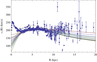
Figure 3: The rotation curves of model galaxies with NFW haloes and exponential thin discs with the parameters listed in Table 3. The data are taken from Sofue et al. (2009). The fit is performed using the datapoints beyond 3 kpc, for which the contribution of non-circular motions caused by the bar is insignificant.

6 Thick Discs

Our methods are also applicable to thick discs, and can give some simple results. As thick discs are predominantly rotationally supported, it makes sense to consider the total kinetic energy rather than the pressure contribution alone. Mass ordering arguments suggest that we discard the contribution of the bulge in the virial relations, even if it is important in shaping the innermost parts of the rotation curve.

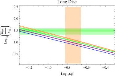
Figure 4: Virial sequences for the thick disc. The equatorial to vertical kinetic energy ratio is shown as a function of the flattening $q$. The thick disc stars move in the potential of a long thin disc and logarithmic halo with relative mass ratio $\mu=0.7$. Each diagonal stripe corresponds to fixing $b={R_{\rm thick}}/{R_{\rm dm}}$ and varying $d={R_{\rm thin}}/{R_{\rm thick}}$ as in Table 2. The vertical and horizontal bands indicate the observationally preferred values of the flattening and the kinetic energy ratio. Notice that all the models lie well below the observational window. [Blue curves are for $b=0.2$, purple for $b=0.25$, green for $b=0.3$ and orange for $b=0.35$. If $\mu$ is increased (decreased), the virial sequences move down (up) in the figure.]

6.1 Formalism

The density profiles of galactic discs tend to be exponential or Gaussian – more complicated than the homogeneous functions used to represent stellar haloes. We shall assume that the thick disc has a double-exponential form:

$$\rho=\rho_{0}\exp\left(-{R\over{R_{\rm thick}}}\right)\exp\left(-{|z|\over z_{\rm h}}\right)$$ (42)

and so the vertical scaleheight $z_{\rm h}=q{R_{\rm thick}}$, where $q$ is as before the axis ratio of the density contours.

Thick discs move in the potential of both the dark halo and thin disc. The latter can be represented by a razor-thin exponential disc with scale-length ${R_{\rm thin}},$ and thus with potential:

$$\Phi_{\rm disc}(R,z)=-2\pi G{R_{\rm thin}}^{2}\Sigma_{0}\int_{0}^{\infty}{\frac{J_{0}(kR)\mathrm{e}^{-k\left|z\right|}}{[1+{R_{\rm thin}}^{2}k^{2}]^{3/2}}}\mathrm{d}k.$$ (43)

The ratio of the kinetic energy tensor components takes the form

$${K_{RR}\over K_{zz}}={\displaystyle\int{\rho R\partial_{R}(\Phi_{\rm disc}+\Phi_{\rm halo})\mathrm{d}^{3}x}\over{\displaystyle\int{\rho z\partial_{z}(\Phi_{\rm disc}+\Phi_{\rm halo})\mathrm{d}^{3}x}}},$$ (44)

and so depends on both the thin disc and halo potentials. By inserting the thick disc density (42) and the thin disc potential (43) into (44), we can find that the disc contributions are

$$D_{R} \propto {\displaystyle\int{\rho R\partial_{R}\Phi_{\rm disc}\mathrm{d}^{3}x}}$$ (45)

$$= \int_{0}^{\infty}{\frac{3k^{2}}{(1+qk)(1+k^{2})^{5/2}(1+k^{2}d^{2})^{3/2}}}\mathrm{d}k\ ,$$

$$D_{z} \propto {\displaystyle\int{\rho z\partial_{z}\Phi_{\rm disc}\mathrm{d}^{3}x}}$$ (46)

$$= \int_{0}^{\infty}{\frac{k}{(1+qk)^{2}(1+k^{2})^{3/2}(1+k^{2}d^{2})^{3/2}}}\mathrm{d}k\ ,$$

where $d={R_{\rm thin}}/{R_{\rm thick}}$. The choice of a double-exponential disc enables the quadruple integrals to be reduced to a single one using formulae [6.623] of Gradshteyn & Ryzhik (1965). This simplification is not possible for general thick-disc density profiles.

Now, let us suppose that the halo is the spherical limit of the logarithmic model

$$\Phi_{\rm halo}=\Phi_{0}\log\left(r^{2}+{R_{\rm dm}}^{2}\right).$$ (47)

Then the halo contributions are

$$H_{R} = b\int_{0}^{\infty}\mathrm{d}\chi\int_{0}^{\infty}\mathrm{d}\xi{\chi^{3}\exp-(\chi+\xi)\over\chi^{2}+q^{2}\xi^{2}+b^{-2}},$$ (48)

$$H_{z} = bq\int_{0}^{\infty}\mathrm{d}\chi\int_{0}^{\infty}\mathrm{d}\xi{\chi\xi^{2}\exp-(\chi+\xi)\over\chi^{2}+q^{2}\xi^{2}+b^{-2}}$$ (49)

where $b={R_{\rm thick}}/{R_{\rm dm}}$. With some careful algebra, we can recast eq. (44) as

$${K_{RR}\over K_{zz}}={1\over q}{2H_{R}+\mu D_{R}\over 2H_{z}+\mu D_{z}}\ ,$$ (50)

where the constant $\mu$ is

$$\mu={2\pi\Sigma_{0}{R_{\rm thin}}^{2}\over\Phi_{0}{R_{\rm dm}}}\ .$$ (51)

In this case, the flattening is not fixed and there is no simple dependence as was the case in the previous sections. The flattening in the total potential is controlled by the $\mu$ parameter, which mediates the contributions of the razor-thin disc and the round dark halo.

As an alternative model for the dark matter potential, we also examine the spherical NFW profile, for which the gravitational force component is

$$\partial_{r}\Phi_{\rm halo} = \frac{4\pi G{\rho_{\rm nfw}}{R_{\rm dm}}^{3}}{r^{2}}\left[\log\left(1\!+\!\frac{r}{{R_{\rm dm}}}\right)-\frac{r}{r\!+\!{R_{\rm dm}}}\right],$$ (52)

$$= \frac{4\pi G{\rho_{\rm nfw}}{R_{\rm dm}}^{3}}{r^{2}}\tilde{\Phi}(r/{R_{\rm dm}}).$$

The disc contributions remain the same, but the halo ones become

$$H_{R} = \int_{0}^{\infty}\!\mathrm{d}\chi\!\int_{0}^{\infty}\mathrm{d}\xi\!{\chi^{3}\exp\!-\!(\chi\!+\!\xi)\over(\chi^{2}+q^{2}\xi^{2})^{3/2}}\tilde{\Phi}({b\sqrt{\chi^{2}\!+\!q^{2}\xi^{2}}})\ ,$$ (53)

$$H_{z} = q\!\int_{0}^{\infty}\!\mathrm{d}\chi\!\int_{0}^{\infty}\mathrm{d}\xi\!{\chi\xi^{2}\!\exp\!-\!(\chi\!+\!\xi)\over(\chi^{2}+q^{2}\xi^{2})^{3/2}}\tilde{\Phi}({b\sqrt{\chi^{2}\!+\!q^{2}\xi^{2}}})\ ;$$ (54)

and the constant $\mu$ is now

$$\mu={\Sigma_{0}{R_{\rm thin}}^{2}\over{\rho_{\rm nfw}}{R_{\rm dm}}^{3}}\ .$$ (55)

In the limit of a massless thin disc $\mu\rightarrow 0$, the ratio $K_{RR}/K_{zz}$ is roughly $\propto q^{-2}$ in the highly flattened limit. This can be deduced from eq. (18) using the conjugateness theorem. Letting the disc become massive, or equivalently introducing a non-vanishing $\mu$, then the rise in pressure deficit for small $q$ is shallower, approximately $\propto q^{-1}$. This is understandable because the presence of a thin disc flattens the total potential, and thus a smaller pressure deficit is required to attain a given tracer flattening when a disc is present.

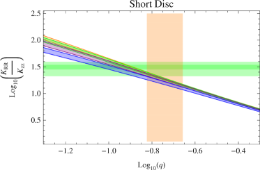
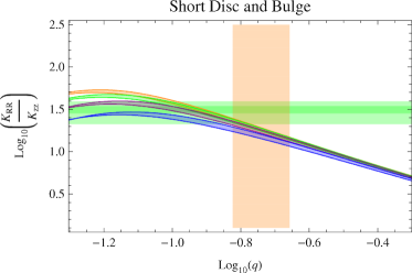
Figure 5: Virial sequences for the thick disc. Left: The thick disc resides in the potential of a short thin disc and logarithmic halo with relative mass ratio $\mu=0.7$. Each diagonal stripe corresponds to fixing $b={R_{\rm thick}}/{R_{\rm dm}}$ and varying $d={R_{\rm thin}}/{R_{\rm thick}}$ as in Table 2. Now all the models cross the observational window, which is the intersection of the vertical orange and horizontal green stripes. Right: The thick disc stars now move in the potential of a short thin disc, a Sersic bulge and a logarithmic halo. Notice that the effects of including the bulge are small in the flattening regime indicated by the observationally preferred orange vertical band. [Blue curves are for $b=1.35$, purple for $b=1.63$, green for $b=1.91$ and orange for $b=2.25$. If $\mu$ is increased (decreased), the virial sequences move down (up) in the figure.]

6.2 Parameter Values

To make progress, we will need to choose astrophysically motivated values for our thick disc models. Here, we are limited by the fact that the thick disc of our Galaxy has not been fully mapped out. We shall see that with the existing data, a rather wide range of parameters is plausible a priori.

De Jong et al. (2010) used SEGUE photometry to find the scalelength of the thick disc ${R_{\rm thick}}=4.1\pm 0.4$ kpc and the scaleheight $z_{\rm h}=0.75\pm 0.07$ kpc. This gives the flattening or axis ratio as

$$q=\frac{0.75\pm 0.07}{4.1\pm 0.4}\approx 0.18\times(1\pm 0.19)\ .$$ (56)

This result is supported by the survey of 34 edge-on galaxies by Yoachim & Dalcanton (2006) who found that thick discs typically have $q=0.18\pm 0.04$.

The velocity dispersions in the thick disc vary with radius, perhaps in a roughly exponential manner (Lewis & Freeman, 1989). The radial variation has not been observationally determined in full, but this does not harm us here. What is important in virial arguments is the ratio of the global averages of horizontal to vertical kinetic energy. This ratio can be well constrained even though the variation of velocity dispersion in the thick disc is not yet fully mapped out. In particular, if the velocity dispersions are proportional to $\sqrt{\rho}$ and therefore vary exponentially, then the ratio of the local averages of horizontal to vertical kinetic energy is equal to the global averages.  This provides some security that using comparatively local measurements of the thick disc velocity dispersions leads to meaningful kinetic energy ratios.

Carollo et al. (2010) explored a local volume within 4 kpc of the Sun and reported that the velocity ellipsoid of the thick disc is $(\sigma_{RR},\sigma_{\phi\phi},\sigma_{zz})=(53\pm 2,51\pm 2,35\pm 1)$ kms^-1 around means of $(\bar{v}_{R},\bar{v}_{\phi},\bar{v}_{z})=(3\pm 2,182\pm 2,0\pm 1$) kms^-1. This gives $K_{RR}/K_{zz}=31.5\times(1\pm 0.06)$. There are also values available from the work of Casetti-Dinescu et al. (2011), who used red clump stars between 5 and 10 kpc of the Galactic Center and between 1 and 3 kpc from the Galactic plane. Stars closer to the Galactic plane are not used to minimize contamination from the thin disc. For the thick disc, they found $(\sigma_{RR},\sigma_{\phi\phi},\sigma_{zz})=(70\pm 4,48\pm 8,36\pm 4)$ kms^-1 around a rotation velocity of $\bar{v}_{\phi}=175\pm 2$ kms^-1. This yields $K_{RR}/K_{zz}=29.2\times(1\pm 0.23)$. Although the values of the dispersions found in the two investigations are not the same, the pressure ratio is much more robust, which adds weight to our argument that the global ratio is well constrained.

The halo and thin disc parameters are of course strongly correlated, as the combined force field must generate the Galactic rotation curve. Sofue et al. (2009, 2010) show that a decomposition into a de Vaucouleurs bulge, exponential disc with spiral arms, and isothermal dark halo gives values of the halo core radius ${R_{\rm dm}}\approx 8-15$ kpc. Sofue et al.’s thin disc has a local surface density of $87M_{\odot}{\rm pc}^{-2}$ and a scalelength ${R_{\rm thin}}=3.5$ kpc – somewhat larger than is found by most other investigators (e.g., Fux & Martinet, 1994; Ojha, 2001; Casetti-Dinescu et al., 2011) – and accordingly we refer to it as the long disc model.

On the other hand, Holmberg & Flynn (2004) used Hipparcos data to measure the local disc surface density as $56\pm 6M_{\odot}{\rm pc}^{-2}$, lower than that estimated by Sofue et al. (2010). Casetti-Dinescu et al. (2011) used kinematical and photometric data to infer the thin disc scale length as ${R_{\rm thin}}=2.6\pm 0.4$ kpc. These observations suggest that the thin disc may be less massive and smaller than advocated by Sofue et al. (2009), and accordingly we refer to this as the short disc model. To fit the rotation curve, this latter model requires lower values of ${R_{\rm dm}}$, accordingly in the range $\approx 1.5-3$ kpc. Of course, this is an underestimate of the true scalelength of the dark matter, as we have not explicitly included a bulge. With these two choices (short versus long disc), the ratios $b$, $d$ and $\mu$ are allowed to vary in the ranges summarized in Table 2. Under the assumption of a logarithmic halo, the mass ratio $\mu$ in the range $\approx 0.7-1.4$ (long disc) and $\approx 0.3-0.7$ (short disc) to provide a reasonable match to the rotation curve. Similarly, the ranges of $b={R_{\rm thick}}/{R_{\rm dm}}$ are constrained to lie in the range $0.25\lesssim b\lesssim 0.56$ (long) and $0.92\lesssim b\lesssim 2.25$ (short). From the scalelengths of the thin and thick discs, we can deduce the range of $d={R_{\rm thin}}/{R_{\rm thick}}$ as $0.78\lesssim d\lesssim 0.95$ (long) and $0.49\lesssim d\lesssim 0.81$ (short).

Matters are more complicated if a NFW profile is chosen for the dark matter potential. Here, we fit the rotation curve data of Sofue et al. (2009) with an exponential disc and NFW halo, as shown in Fig. 3. Even keeping the local disc density as $56M_{\odot}{\rm pc}^{-2}$ and ${R_{\rm thin}}\gtrsim 2.4$ kpc, there is quite a large range in which the other parameters may vary. We list the parameters of the models in Table 3, although we shall show that their virial sequences are not too different.

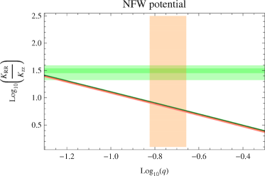
Figure 6: As Fig. 5, but for a NFW rather than the logarithmic halo. Plotted are all the virial sequences for the models with rotation curves displayed in Fig. 3. Different colours stand for different values of $b={R_{\rm thick}}/{R_{\rm thin}}$, but the sequences are so near to one another that listing the colour correspondence is superfluous.

6.3 Short versus Long Thin Discs

Our method is to take ${R_{\rm thick}}=4.1\pm 0.4$ kpc from de Jong et al. (2010) and ${R_{\rm thin}}$ either short at $2.6\pm 0.4$ kpc (Casetti-Dinescu et al (2011) or long at 3.5 kpc from Sofue et al (2009). Then a fit to Sofue’s data – as judged by the likelihood falling to half its maximum value – is used to find plausible ranges of $d$ and $\mu$ . Virial sequences are found by fixing $b$, and $\mu=0.7$, then varying $q$ to get a single line across the plane, and finally $d$ (within the range found from the rotation curve) to get a band of finite width rather than a single line.

The panels of Figs 4 and 5 show such virial sequences. They give the thick disc kinetic energy ratio as a function of flattening $q$. The allowed observational range is shown by vertical and horizontal stripes, so that the intersection gives the region compatible with the data. Specifically, the vertical orange stripe corresponds to the flattening of the thick disc inferred by de Jong et al. (2010), whilst the horizontal green stripes correspond to the kinetic energy ratios from Carollo et al. (2010) and Casetti-Dinescu et al. (2011).

Plotted on Figs 4 and  5 are the virial sequences of the long and short discs respectively. We see that the short disc does indeed give a better match to the observations than the long disc, even when the $\mu$ parameter is taken towards the high end of its possible range. By contrast, the virial sequences for the long disc yield pressure ratios that lie appreciably below the estimated ones, for all the relevant values of $\mu$ parameter.

The effects of incorporating a bulge are shown in the right panel of Fig 5. The fit to the rotation curve is performed again, using a short thin disc, an isothermal dark halo and a spherical Sersic $m=3$ bulge, given by the deprojection of

$$\Sigma(R)=\Sigma_{0}\exp\left(-\kappa(R/R_{\rm e})^{1\over 3}\right)$$ (57)

Here, $\Sigma$ is the projected bulge density on the sky, $R$ is projected radius and $R_{\rm e}$ is the effective radius and $\kappa$ is a constant. The values of the parameters are chosen to give a total bulge mass of $\sim 10^{10}M_{\odot}$ and a maximum contribution to the rotation curve of $\sim 100$ kms^-1. The parameter values are suggestive rather than definitive, as we merely wish to ascertain the importance of the effect. In fact, we notice that the virial sequences do not change much in the observational regime – the left and right panels of Fig. 5 are very similar for $q\gtrsim 0.1$. This is understandable, as the models with or without a bulge reproduce the same overall rotation curve, albeit using different components. The virial quantities do not change much, as they depend on the total potential.

We conclude that the flattening and kinematics of the thick disc are consistent with stellar motion in a potential generated by a thin disc with a short scalelength $\sim 2.6$ kpc, together with the normalisation suggested by Holmberg & Flynn (2004). In particular, thin discs with longer scalelengths $\sim 3.5$ kpc are necessarily more massive if they are to reproduce the local surface density. The stronger gravity field towards the equatorial plane then causes the thick disc to be flatter than is measured, given the observed kinematics.

We briefly show the differences made by using a NFW halo rather than a logarithmic one in Fig. 6. Here, all the virial sequences corresponding to the parameters in Table 3 lie below the observational estimates for flattening versus pressure excess. The reason for this is as follows. For cusped potentials, the virial terms are dominated by contributions from near the central cusp. Near the very centre, the combined equipotentials due to the thin disc and spherical halo are flatter than the tracer density. If this region is weighted more in the virial integrals, then the average $K_{zz}$ required to produce the flattening is greater and so the virial sequences of an NFW halo fall below those of a logarithmic halo and also the observational data (cf. Figs. 5 and 6). Thus, a logarithmic potential with a finite core seems to be favoured over an NFW profile, at least as judged from the present constraints on the thick disc kinematics.

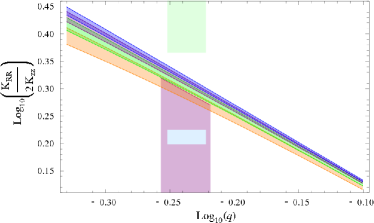
Figure 7: Virial sequences for the stellar halo in a spherical logarithmic dark halo plus a short thin disc. The relative weighting of the disc and halo is controlled by $\mu=0.7$. Each virial sequence corresponds to fixing ${\hat{b}}={R_{\rm b}}/{R_{\rm dm}}$ and varying ${\hat{d}}={R_{\rm thin}}/{R_{\rm b}}$ from 0.09 to 0.12 (see text). The models all lie above the pale blue Smith et al. (2009a) databox. Lower values of $\mu$ yield somewhat higher pressure ratios, but still below the pale green Kepley et al. (2007) databox. The purple shaded zone shows models with constant anisotropy and spherical alignment, with the extreme radial orbit model providing the diagonal edge. [Blue curves are for $b=7$, purple for $b=8.6$, green for $b=10.2$ and orange for $b=12$.]

7 The Stellar Halo Revisited

In Section 5, we presented a simple model of the stellar halo, and showed that if the local measurements of the velocity dispersion using the SDSS subdwarfs (Smith et al. 2009a) are a good guide to the global kinematics, then this implies a moderately flattened potential with an axis ratio of $g\approx 0.85$. If this is ascribed solely to the dark matter halo, then it corresponds to a flattening in the dark matter density contours of $\approx 0.7$.

In Section 6, we showed that the global kinematics of the thick disc are consistent with motion in the combined potential of a spherical dark halo together with a thin disc. Here, we will ask: is it possible that the dark halo is spherical, and that the flattening in the potential measured from the kinematics of halo stars is due entirely to the presence of the thin disc? If the dark halo is round, then the flattening of the combined disc and halo equipotentials changes from $\approx 0.5$ close to the Galactic centre to $\approx 1$ at Galactocentric distances beyond 10 kpc.

The gravity field is now provided by the thin disc potential with short scalelength $\sim 2.6$ kpc, together with a completely spherical logarithmic dark matter potential as in eq (47). The stellar halo density is given by the broken power-law of eq (39) with break radius ${R_{\rm b}}$. The two lengthscales involved are

$${\hat{b}}=\frac{{R_{\rm b}}}{{R_{\rm dm}}}\qquad\qquad{\hat{d}}=\frac{{R_{\rm thin}}}{{R_{\rm b}}},$$ (58)

We compute virial sequences for ${\hat{b}}$ in the range 7 to 14 and ${\hat{d}}$ in the range 0.09 to 0.12, which are suggested by the roughly known values of the scalelengths (that is, ${R_{\rm thin}}=2.6\pm 0.4$ kpc, ${R_{\rm b}}\approx 2$ - $4$ kpc and ${R_{\rm b}}\approx 27$ kpc)

Fig. 7 shows the pressure ratio $\Pi_{RR}/\Pi_{zz}$ as a function of $q$, the flattening of the stellar halo. The light blue and green boxes indicate the observational regimes, depending on whether the pressure ratio is estimated from the data of Smith et al. (2009a) or of Kepley et al. (2007) assuming cylindrical alignment. In each case, the constraints on flattening come from the work of Deason et al. (2011b). The virial sequences lie below the Kepley et al. (2007) databox and above the Smith et al. (2009a) databox. Accordingly, it seems reasonable to argue that the underlying assumption of a spherical dark halo may hold good, as the models are not too far off the uncertain data. The purple zone covers the parts of the ($\Pi_{RR}/\Pi_{zz},q$) plane for which the velocity ellipsoid is spherically aligned and the anisotropy is constant using eq (27). The upper diagonal line corresponds to the purely radial orbit model. Hence, the models that do reproduce the observations are radially biased with an anisotropy parameter $\beta\approx 0.9$. This makes good sense, as the underlying dark halo is nearly spherical at large radii where the disc becomes unimportant, in which case the flattening can only be produced by substantial radial anisotropy. However, such radial anisotropy is much more extreme than implied by Kepley et al.’s (2007) or Smith et al’s (2009a) data, which have $\beta\approx 0.6$.

8 Conclusions

The tensor virial theorem can provide a powerful technique for extracting gross structural properties, such as flattenings, from datasets. It has been widely used in galactic astronomy, particularly for self-gravitating systems – such as stars in elliptical galaxies — moving in the potential generated by their density field. The literature on applications to tracer populations, in which the stars are primarily moving in the gravity field provided by dark matter or other stellar components, is quite sparse (White, 1989; Sommer-Larsen & Christensen, 1989; Helmi, 2008).

We have provided the first systematic exploitation of the tensor virial theorem for tracer stellar populations, and shown how it can be used to yield constraints on global kinematics and flattening. This technique offers considerable advantages over, for example, the Jeans equations. The latter depend on the derivatives of densities and velocity dispersions, and are necessarily subject to uncertainties with noisy data. The tensor virial theorem deals with integrated bulk quantities, which are less susceptible to observational errors or systematic problems such as substructure in the data.

An obvious application is to Population II stars moving in the dark halo of our Galaxy. For spheroidal tracer populations with flattening $q$ moving in spherical power-law potentials, there are analytic results that prescribe the ratio of globally averaged equatorial to vertical velocity dispersion. Thanks to the Flattening Theorem, the results can be straightforwardly adapted to spheroidal dark halos with axis ratio $g$ in the equipotentials. The virial quantities depend only on the ratio $q/g$ in this instance.

The main astrophysical results of the paper are threefold. First, we have shown how to interpret the stellar kinematical measurements of halo stars in terms of the global flattening of the dark halo. In particular, if the Smith et al. (2009a) values for the velocity dispersion of the halo subdwarfs are accepted, then the dataset is consistent with oblate dark halo models with a flattening in the potential of $g\approx 0.85$, corresponding to a flattening in the dark matter density contours of $\approx 0.7$; this is driven by the radial anisotropy that Smith et al. found. If however, the Kepley et al. (2007) values are preferred, then the dark halo may well be close to spherical. We have to make the assumption that the local kinematics are proxies for the global kinematics, which is assuredly a weakness in such analyses at present. However, the GAIA satellite, which is scheduled to fly in 2013, will for the first time provide us with detailed information on the three-dimensional kinematics of halo stars, and so there is hope for real advances using this technique in the near future.

Secondly, we have demonstrated that the dual halo structure as proposed by Carollo et al. (2010) appears to be incorrect. It is not possible to support an inner halo and an outer halo with the claimed velocity dispersions in the same gravitational potential: the model is inconsistent with the requirements of the virial theorem. A powerful aspect of virial methods is the fact that multiple populations residing in the same potential can be used to cross-constrain the dark hark halo mass and shape, without the need of building detailed models to reproduce the photometry and kinematics. There is considerable scope for extending our virial techniques to study multiple populations moving in the same gravity field, a topic that is already important in studies of the dwarf spheroidals (Amorisco & Evans, 2011; Walker & Penarrubia, 2011).

Thirdly, we have carried out an investigation into the kinematics of the thick disc. We find that the reported thick disc kinematics are consistent with a thin disc with scalelength and an isothermal dark halo. Specifically, we find that the thick disc kinematics and shape is consistent with a potential generated by a thin disc with scalelength $\approx 2.6$ kpc, and surface-density normalisation of $56\pm 6M_{\odot}{\rm pc}^{-2}$ (Holmberg & Flynn, 2004). Although NFW potentials can be used to fit the rotation curve, they seemingly fail to reproduce the virial ratios expected for the thick disc, as judged from the observational data.

The near future sees a number of ambitious radial velocity surveys, such as ESO-GAIA and Hermes. These will complement the abundant positional and proper motion data on stars in the Galaxy that will be delivered by the GAIA satellite. Given the quality and quantity of the datasets, it is an attractive proposition to look at virial quantities to gain insight into the Galaxy’s potential, perhaps as a prelude to detailed phase space modelling. We anticipate that the tensor virial theorem will become an important tool to make sense of the very large datasets on stellar positions and velocities that will become available in the future.

References

- Amorisco & Evans (2011) Amorisco N., Evans N.W., 2011, MNRAS, in press.
- An et al. (2004) An, J. H., et al. 2004, MNRAS, 351, 1071
- Battaglia et al. (2005) Battaglia, G., Helmi, A., Morrison, H., et al. 2005, MNRAS, 364, 433
- Bell et al. (2008) Bell, E. F., et al. 2008, ApJ, 680, 295
- Binney (1978) Binney, J. 1978, MNRAS, 183, 501
- Binney (1981) Binney, J. 1981, MNRAS, 196, 455
- Binney (2005) Binney, J. 2005, MNRAS, 363, 937
- Bramich et al. (2008) Bramich, D. M., et al. 2008, MNRAS, 386, 887
- Carollo et al. (2007) Carollo, D., et al. 2007, Nat, 450, 1020
- Carollo et al. (2010) Carollo, D., et al. 2010, ApJ, 712, 692
- Casetti-Dinescu et al. (2011) Casetti-Dinescu, D. I., Girard, T. M., Korchagin, V. I., & van Altena, W. F. 2011, ApJ, 728, 7
- Chandrasekhar (1987) Chandrasekhar S. 1987, Ellipsoidal Figures of Equilibrium, Dover
- Ciotti & Morganti (2010) Ciotti, L., & Morganti, L. 2010, MNRAS, 408, 1070;
- de Jong et al. (2010) de Jong, J. T. A., Yanny, B., Rix, H.-W., et al. 2010, ApJ, 714, 663
- Deason et al. (2011a) Deason, A. J., Belokurov, V., & Evans, N. W. 2011a, MNRAS, 411, 1480
- Deason et al. (2011b) Deason, A. J., Belokurov, V., & Evans, N. W. 2011b, MNRAS, 416, 2903
- Evans (1993) Evans, N. W. 1993, MNRAS, 260, 191
- Evans (1994) Evans, N. W. 1994, MNRAS, 267, 333
- Evans et al. (1997) Evans, N. W., Hafner, R. M., & de Zeeuw, P. T. 1997, MNRAS, 286, 315
- Fux & Martinet (1994) Fux, R., & Martinet, L. 1994, AA, 287, L21
- Gradshteyn & Ryzhik (1965) Gradshteyn I.S., Ryzhik I.M. 1965, Tables of Integrals, Series and Products, Academic Press, New York.
- Helmi (2008) Helmi, A. 2008, AA Rev, 15, 145
- Holmberg & Flynn (2004) Holmberg, J., & Flynn, C. 2004, MNRAS, 352, 440
- Kepley et al. (2007) Kepley, A. A., et al. 2007, AJ, 134, 1579
- Lewis & Freeman (1989) Lewis, J. R., & Freeman, K. C. 1989, AJ, 97, 139
- Navarro et al. (1996) Navarro, J. F., Frenk, C. S., & White, S. D. M. 1996, ApJ, 462, 563
- Ojha (2001) Ojha, D. K. 2001, MNRAS, 322, 426
- Petrou (1981) Petrou, M., 1981, PhD Thesis, University of Cambridge
- Roberts (1962) Roberts, P.H. 1962, ApJ, 136, 1108
- Sérsic (1963) Sérsic, J. L. 1963, Boletin de la Asociacion Argentina de Astronomia La Plata Argentina, 6, 41
- Sesar et al. (2011) Sesar, B., Jurić, M., & Ivezić, Ž. 2011, ApJ, 731, 4
- Smith et al. (2009a) Smith, M. C., et al. 2009a, MNRAS, 399, 1223
- Smith et al. (2009b) Smith, M. C., Evans, N.W., An, J. H. 2009b, ApJ, 698, 1110
- Sluis & Arnold (1998) Sluis, A. P. N., & Arnold, R. A. 1998, MNRAS, 297, 732
- Sofue et al. (2009) Sofue, Y., Honma, M., & Omodaka, T. 2009, PASJ, 61, 227
- Sofue et al. (2010) Sofue, Y., Honma, M., & Omodaka, T. 2010, PASJ, 62, 1367
- Sommer-Larsen & Christensen (1989) Sommer-Larsen, J., & Christensen, P. R. 1989, MNRAS, 239, 441
- van der Marel (1991) van der Marel, R. P. 1991, MNRAS, 253, 710
- Walker & Penarrubia (2011) Walker M. G., Penarrubia J., 2011, ApJ, in press
- Watkins et al. (2009) Watkins, L. L., et al. 2009, MNRAS, 398, 1757
- Watkins et al. (2010) Watkins, L. L., Evans, N. W., & An, J. H. 2010, MNRAS, 406, 264
- White (1989) White, S. D. M. 1989, MNRAS, 237, 51P
- Yanny et al. (2009) Yanny, B. et al. 2009, AJ, 137, 4377
- Yoachim & Dalcanton (2006) Yoachim, P., & Dalcanton, J. J. 2006, AJ, 131, 226